Sage Journals: Discover world-class research

Abstract

This article proposed a computational workflow for city-scale building damage estimation based on broadband physics-based ground motion simulation. The dynamic stiffness matrix method in frequency-wavenumber domain is employed for broadband physics-based ground motion simulation of finite fault along with site response correction using equivalent-linear site response analysis approach. With simulated ground motion, seismic response of buildings, using multi-degree of freedom model, is simulated using nonlinear time history analysis, and building damage is evaluated based on a trilinear backbone curve of story’s nonlinear force-drift model. Main advantage of the framework lies in the employed dynamic stiffness matrix method for ground motion simulation, which can efficiently generate broadband ground motions in perfect parallel and naturally capture the physics of finite fault source, propagation path, and spatial variability characteristics of ground motion. To demonstrate the salient features of proposed workflow, the 2021 M_s 6.4 Yangbi earthquake is simulated with frequency resolution up to 20 Hz, and seismic damage of buildings in Yangbi county are estimated. Results show that most traditional wood-adobe structures suffer moderate to severe damage, and engineered seismic buildings (mostly RC frame) in Yangbi county suffer minor damage, which agrees with field investigation results.

Keywords

Physics-based ground motion simulation dynamic stiffness matrix method damage estimation city-scale buildings Yangbi earthquake

Introduction

Modern cities are densely distributed with residence, office, and commercial buildings, and it seems that their development and expansion will continue in future decades. However, big earthquakes that happen near cities might lead to devastating casualties and economic loss, for example, the 2008 Wenchuan earthquake (Zeng and Wang, 2013), 2011 Fukushima earthquake (Mimura et al., 2011), and 1994 Northridge earthquake (Norton et al., 1994). Therefore, accurate prediction of seismic damage and loss on a city scale is vital for providing valuable strategies for the emergency rescue team to respond quickly and effectively after the earthquake, for policymakers to make plans for earthquake reconnaissance project.

Existing approaches for city-scale seismic damage prediction mainly include three methods: damage probability matrix method (Applied Technology Council (ATC), 1985), capacity spectrum method (Federal Emergency Management Agency (FEMA), 2012), and nonlinear time history analysis method (Hori, 2006). Damage probability matrix method, based on data collected from past earthquakes, is heavily dependent on data availability and expert judgment. Although it is quite straightforward for engineers to implement into practice, it is not reliable for areas with limited historical data. Detailed procedures to develop damage probability matrices can be referred to the work by Eleftheriadou and Karabinis (2011). The capacity spectrum method, through a static pushover analysis of single-degree-of-freedom building model, compares structural capacity in terms of pushover curve with structural demand in terms of response spectra (Barbat et al., 2008). It could well represent the strength and ductility of buildings, but seismic response from higher structural modes is neglected due to the employment of single-degree-of-freedom model. In addition, dynamic effects driven by the ground motion are also difficult to capture due to the limitation of static pushover analysis. Example of capacity spectrum method applications and its improvements can be found in the works by Gencturk and Elnashai (2008), Nettis et al. (2021), and Peter and Badoux (2000).

With the rapid development of computer hardware, nonlinear time history analysis of structure is commonly employed among researchers and engineers. Hori and Ichimura (2008) proposed an integrated earthquake simulation (IES) system based on nonlinear time history analysis. Lu et al. (2020) proposed an open-source framework for earthquake loss estimation using city-scale nonlinear time history analysis, and developed a program RED-ACT for rapid earthquake damage simulation (Lu et al., 2019). In addition, detailed procedures to determine model parameters are also presented for the framework (Xiong et al., 2017). Lin et al. (2019) developed a simulation platform called YouSimulator, which integrates modeling, nonlinear time history analysis, damage evaluation, and visualization, and superb efficiency is achieved by using parallel computing, for instance, analysis with about 1 million buildings can be completed in 10 min. Recently, Zhang et al. (2023a) developed a three-dimensional (3D) nonlinear time history analysis procedure by automatically calling open-source software OpenSees to perform realistic 3D simulations of city-scale structures.

Although refined models with judiciously calibrated parameters could achieve considerable accuracy in city-scale earthquake damage simulation, uncertainties remain as spatial-temporal variability of ground motion is usually ignored by using a single record as ground motion input for city-scale structures (Jayaram and Baker, 2009; Smerzini and Pitilakis, 2018). To overcome this limitation, physics-based ground motion simulation, by explicitly modeling the ruptured fault, wave propagation path, could generate synthesized seismograms to capture the spatial-temporal variability characteristics. Smerzini and Pitilakis (2018) performed a physics-based ground motion simulation of the 1978 M_w 6.5 Volvi earthquake and employed the capacity spectrum method to evaluate building damage in the city of Thessaloniki, Greece. Antonietti et al. (2021) performed a seismic risk assessment for the Beijing metropolitan area based on physics-based simulation results and empirical fragility functions to evaluate structure damage. McCallen et al. (2021) proposed an EQSIM framework for fault-to-structure simulations enhanced with high-performance computing, which could include complex topography, surface soil nonlinearity, and so on. Kenawy et al. (2021) evaluated the variability of near-fault seismic risk to RC buildings using physics-based ground motion simulations.

However, broadband ground motion simulation for engineering structures, which requires 10 Hz or more, is still computationally challenging, and simulation time increases drastically with increased frequency resolution. Hybrid approaches are usually adopted to use stochastic methods to generate high-frequency components of motion and combine them with low-frequency motion from physics-based simulation to generate broadband seismic motions (Mai et al., 2010; Paolucci et al., 2018). Distinct from the hybrid methods, the author of this article has developed a dynamic stiffness matrix method in the frequency-wavenumber (FK) domain (Ba et al., 2021, 2022), which could simulate seismic wave propagation problems of layered half-space with kinematic finite fault. Based on computed Green functions between the source and observation point, the computing requirement of the dynamic stiffness matrix method increases linearly with increasing frequency resolution demand, which is advantageous over exponential increase for finite element, spectral element, and so on.

Therefore, this article integrates the efficient dynamic stiffness matrix method for physics-based broadband ground motion simulations with city-scale nonlinear time history analysis for seismic damage estimation and damage simulation for Yangbi county, Yunnan, China under 2021 M_s 6.4 Yangbi earthquake is performed as a case study. The novelty of this article mainly lies in the integration of efficient dynamic stiffness matrix method for broadband ground motion simulation of finite fault with regional buildings damage estimation, which could relieve the computational burden of physics-based earthquake simulations. The dynamic stiffness matrix method in the FK domain could be run perfectly parallel for ground motion simulation in the context of multiple observation points (suitable for city-scale damage estimation). Observation points, namely, building locations, could be separated into independent groups and run in different workstations or multiple nodes of a computing center. In addition, site response correction is performed using equivalent-linear site response to account for site effects. Note that the employed dynamic stiffness matrix method only works for layered medium. For complex models with topography, more advanced numerical methods, finite element, spectral element, and finite difference, should be used. Typical applications of these advanced methods on ground motion simulations can be found in the works by Zhang et al. (2021b, 2023b), McCallen et al. (2021), and Kenawy et al. (2021).

In the following section, we describe the details of the hybrid finite-fault source model of 2021 M_s 6.4 Yangbi earthquake, formulation of the dynamic stiffness matrix method, site response correction procedure, and simulated ground motions are verified with eight typical station records. Subsequently, we present the inventory of 2216 buildings in urban area of Yangbi county, and discuss the damage estimation results based on simulated ground motion in the previous section. Finally, some concluding remarks and implications from this study are summarized. Figure 1 presents the computation workflow of the city-scale damage estimation based on ground motion simulation using the dynamic stiffness matrix method.

Figure 1.

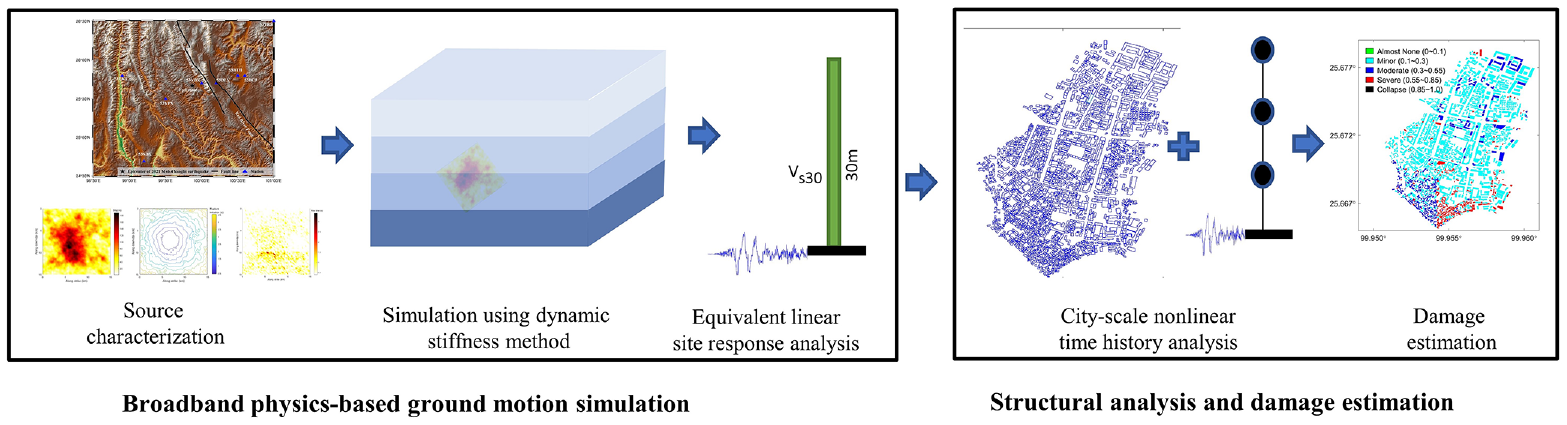
Computational workflow for city-scale buildings damage estimation based on physics-based ground motion simulation.

Broadband ground motion simulations of 2021 M_s 6.4 Yangbi earthquake

The 2021 M_s 6.4 Yangbi earthquake with moment magnitude 6.1 occurred at the intersection of the Red River and Weixi-Qiaohou-Weishan faults, in a region of western Yunnan Province with complex mountain topography (see Figure 2). It is the largest earthquake occurred in this region in the past 45 years (Wang et al., 2023). Epicenter of this strike-slip earthquake is located at latitude 25.67°N, longitude 99.87°E. The earthquake was well recorded by 28 National Strong Motion Observation Network System (NSMONS) stations in China. Note that most of these seismic records are far-field records, and near-field records are rare. The largest records among them are the 53YBX station record with peak ground accelerations 0.34 g, 0.70 g, 0.26 g in EW, NS, UD directions, respectively. The original records are corrected using a fourth-order Butterworth bandpass filter with a low frequency of 0.05 Hz and a high frequency of 20 Hz. This article selects eight station records (53YBX, 53DLY, 53YPX, 53BTH, 53BCJ, 53LKT, 53SDX, 53YRH) for validations of our broadband ground motion simulation of the Yangbi earthquake, which will be discussed later in this section.

Figure 2.

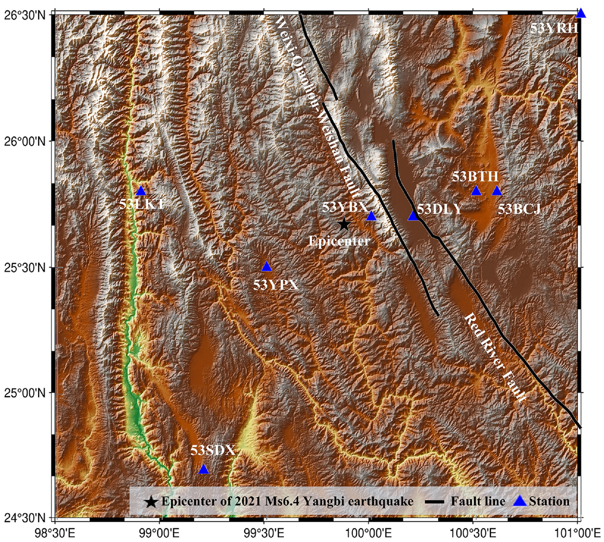
Epicenter location, fault distribution, nearby recording stations for 2021 M_s 6.4 Yangbi earthquake.

Establishment of the hybrid kinematic fault model

The kinematic fault model requires the fault location, fault geometry (length, width, strike, dip, rake), rupture initiation point, slip distribution, rupture initiation time, and rise time of all subfaults. According to the focal mechanism studies of the 2021 Yangbi earthquake by the United States Geological Survey (USGS; https://earthquake.usgs.gov/earthquakes/eventpage/us7000e532/moment-tensor), the ruptured fault plane has a strike angle of 135°, dip angle of 82°, rake angle of −165°. Based on the work by Zhang et al. (2021a), the fault plane in our article is employed as a square with width of 15 km on each side, and the average slip is 40 cm on the rupture plane. Top of the fault plane is 3 km deep from the surface.

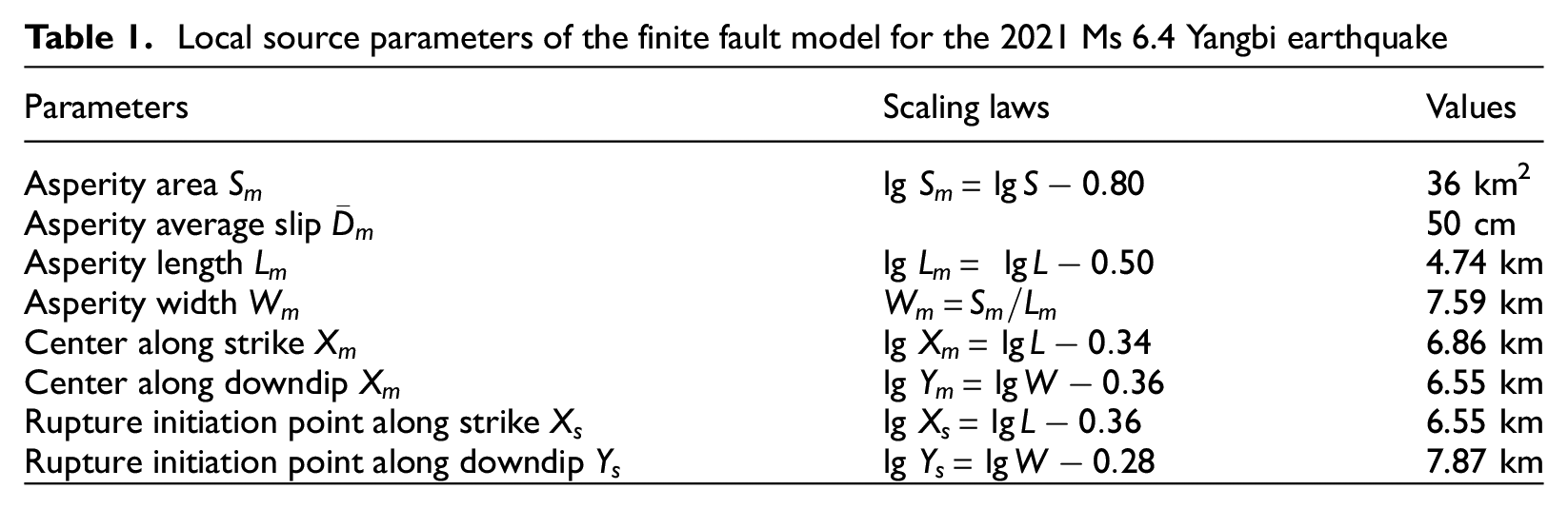
To incorporate inhomogeneity and roughness of slip distribution on the rupture plane, a single asperity is used to estimate the local source parameters. By using the empirical scaling laws from the work by Jiang et al. (2021), the local source parameters are determined in terms of the global source parameters. Although empirical scaling law for asperity average slip exists, it is important to calibrate the slip distribution with latest source inversion studies of Yangbi earthquake. Source studies on Yangbi earthquake suggest a max slip around 60 cm (Wang et al., 2022; Zhu et al., 2022), and an asperity average slip of 50 cm is used in this study. The determined local source parameters are listed in Table 1.

Table 1.

Local source parameters of the finite fault model for the 2021 Ms 6.4 Yangbi earthquake

Parameters	Scaling laws	Values
Asperity area $S_{m}$	$\lg S_{m} = \lg S - 0.80$	36 km²
Asperity average slip ${\bar{D}}_{m}$		50 cm
Asperity length $L_{m}$	$\lg L_{m} = \lg L - 0.50$	4.74 km
Asperity width $W_{m}$	$W_{m} = S_{m} / L_{m}$	7.59 km
Center along strike $X_{m}$	$\lg X_{m} = \lg L - 0.34$	6.86 km
Center along downdip $X_{m}$	$\lg Y_{m} = \lg W - 0.36$	6.55 km
Rupture initiation point along strike $X_{s}$	$\lg X_{s} = \lg L - 0.36$	6.55 km
Rupture initiation point along downdip $Y_{s}$	$\lg Y_{s} = \lg W - 0.28$	7.87 km

To introduce high-frequency component of the simulated seismic motion, the Graves and Pitarka (2010, 2015) approach, also named as GP14.3, is employed. It assumes random phases in the transformed wavenumber domain to achieve a roughly wavenumber-squared spectral decay of the slip distribution. In addition, it adds random perturbations to rupture initiation time and local rise time to remove 1:1 correlation with local slip. In the end, spatial heterogeneity of slip distribution, rupture initiation and rise time is developed for the kinematic fault model to produce broadband seismic motions.

The fault plane for the 2021 M_s 6.4 Yangbi earthquake is divided into 30 segments in each direction, which results in a total of 900 subsources. By applying the GP14.3 model, slip distribution, rupture initiation time, and rise time of all subsources of the kinematic fault are generated and shown in Figure 3. Evident scattering on the slip distribution is achieved, and rupture initiation propagates away with varying speed in all directions. As the employed fault size is smaller than those proposed by source studies (Wang et al., 2022; Zhu et al., 2022), the maximum slip is around 80 cm which is a bit larger than 60 cm from them. In addition, note that rise times of lower part subsources are generally shorter than those in the upper part, which conforms with higher rupture speed in the lower part of the fault.

Figure 3.

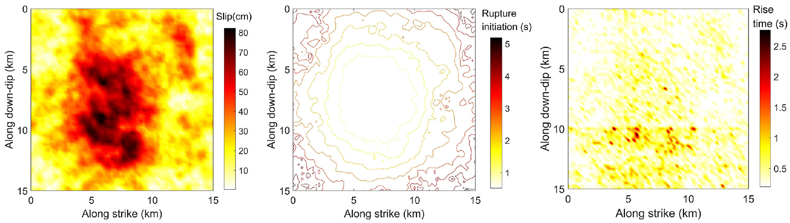
Slip distribution, rupture initiation time, and rise time of the kinematic fault model for the 2021 M_s 6.4 Yangbi earthquake.

Earthquake simulations using dynamic stiffness matrix method

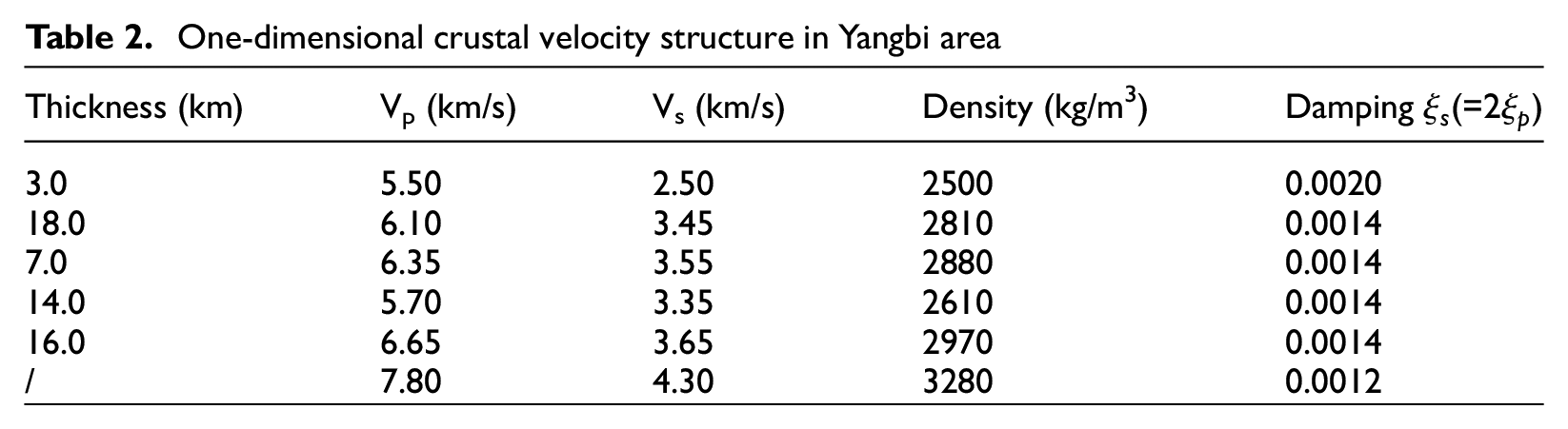
The propagator matrix method is originally proposed by Thomson (1950) and Haskell (1953), and further improved by many researchers, for instance, Knopoff (1964) and Kausel and Roesset (1977). On the other hand, the dynamic stiffness matrix method employed in this article is first derived by Wolf (1985) in two dimensions (2D), and extended to 3D by the authors (Liang and Ba, 2007). Then, we formulated the dynamic stiffness matrix with point source representation in a frequency-wavenumber domain to simulate the wave propagation due to point seismic sources in layered half-space (Ba et al., 2021, 2022), and synthesized seismic motions in the spatial-temporal domain can be acquired through inverse Fourier–Hankel transformation. As the finite fault can be divided into a certain number of subsources, that is, point sources, the dynamic stiffness matrix method applies to the simulation of 2021 M_s 6.4 Yangbi earthquake, which is an extended work based on previous point source modeling (Ba et al., 2021, 2022). Table 2 lists information of the crustal velocity structure in Yangbi area according to Li et al. (2021b). As Li et al. (2021b) only present V_p, V_s, and density values, the damping in Table 2 is estimated by $ξ_{s} = 1 / (2 Q_{s})$ with quality factor Q_s = V_s/10. Formulation of the dynamic stiffness matrix method is briefly introduced here, and detailed derivations can be found in the work by Ba et al. (2022).

Table 2.

One-dimensional crustal velocity structure in Yangbi area

Thickness (km)	V_p (km/s)	V_s (km/s)	Density (kg/m³)	Damping $ξ_{s}$ (=2 $ξ_{p}$ )
3.0	5.50	2.50	2500	0.0020
18.0	6.10	3.45	2810	0.0014
7.0	6.35	3.55	2880	0.0014
14.0	5.70	3.35	2610	0.0014
16.0	6.65	3.65	2970	0.0014
/	7.80	4.30	3280	0.0012

For a layered half-space, the construction of global dynamic stiffness matrix relies on the assembly of each layer’s stiffness matrix, which is similar to matrix assembly procedure in finite element theory. For a specific layer i, the equilibrium equation, in frequency-wavenumber (FK) domain, can be written as follows:

{{\bar{P}}_{1}^{(i)}, i {\bar{R}}_{1}^{(i)}, {\bar{P}}_{2}^{(i)}, i {\bar{R}}_{2}^{(i)}, {\bar{Q}}_{1}^{(i)}, {\bar{Q}}_{2}^{(i)}}^{T} = [\begin{matrix} K_{P - SV}^{(i)} \\ K_{SH}^{(i)} \end{matrix}] {{\bar{u}}_{1}^{(i)}, i {\bar{w}}_{1}^{(i)}, {\bar{u}}_{2}^{(i)}, i {\bar{w}}_{2}^{(i)}, {\bar{v}}_{1}^{(i)}, {\bar{v}}_{2}^{(i)}}^{T}

(1)

where $K_{P - SV}^{(i)}$ , $K_{SH}^{(i)}$ denote the dynamic stiffness matrices for in-plane motion and out-of-plane motion of layer i, respectively. External load in in-plane horizontal, in-plane vertical, out-of-plane directions are denoted as P, R, and Q, respectively. Similarly, u, w, and v denote the displacement amplitude in three directions at the two-layer interfaces subscripted with 1 and 2. Symbol “—” on top of a variable denotes the FK domain of the variable.

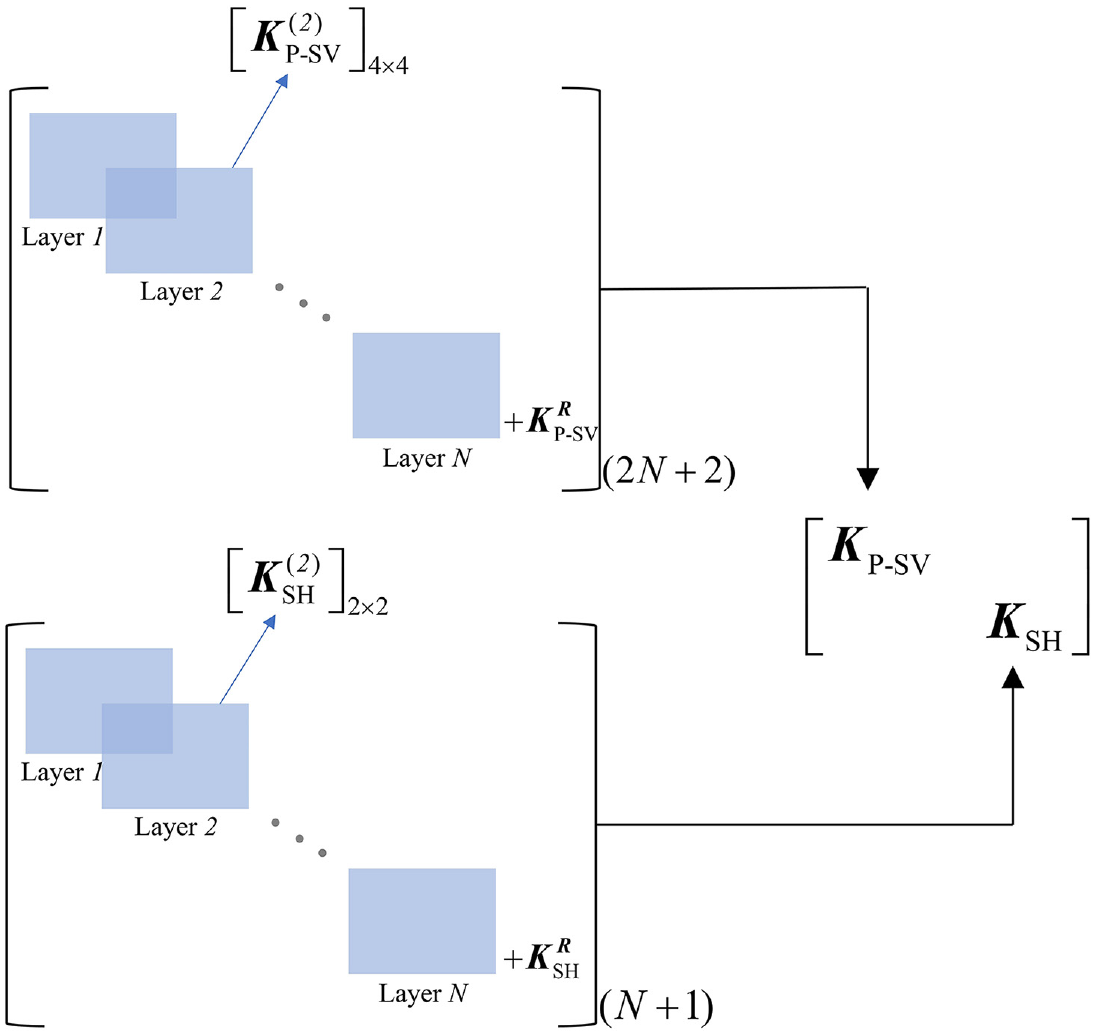
As the in-plane stiffness matrix and out-of-plane stiffness matrix are decoupled per Equation 1, the global stiffness matrix with N number of layers can be assembled separately, as shown in Figure 4. Note that $K_{P - SV}^{R}$ , $K_{SH}^{R}$ represent the in-plane and out-of-plane stiffness matrix of the half-space.

Figure 4.

Illustration on assembly of global dynamic stiffness matrix in FK domain.

For a point seismic source, its moment tensor M could be converted to equivalent body force F as:

F = \nabla [M δ (r - r_{S}) δ (z - z_{S})]

(2)

where δ denotes the Dirac delta function, r_s and z_s denote the two horizontal and one vertical coordinates of the point source, ▽ is a Nabla-difference operator working as ▽ e = e _{r, r} + r^-1 e _θ,θ + e _{z, z}, and e _r, e _θ, e _z represent the unit vectors in three orthogonal cylindrical directions. To decouple the equivalent body force, we introduce a set of orthogonal bases ${R_{k}^{m}, S_{k}^{m}, T_{k}^{m}}$ for vector harmonic expansions.

To establish the Green function of the point source, three steps should be followed: First, fix the top and bottom interfaces with the source, and compute the reaction forces P _m at two interfaces; Second, release the two interfaces and apply the computed reaction forces in an opposite direction, solve for the dynamic displacement response using the dynamic stiffness matrix (Equation 3); Finally, use vector surface harmonics to couple the dynamic displacement response due to the point source, and convert to displacement response in spatial-temporal domain using inverse Fourier–Hankel transformation (Equation 4).

K U_{m} = P_{m}

(3)

u = \int_{- \infty}^{\infty} e^{i ω t} dt \int_{0}^{\infty} \sum_{m = - 2}^{m = + 2} [u_{m} S_{m}^{k} + v_{m} T_{m}^{k} + w_{m} R_{m}^{k}] e^{im θ} kdk

(4)

The acquired dynamic displacement response u (Equation 5) is actually the displacement Green function g(x, t) between the point source and observation point.

For a finite fault divided into a number of subsources, the seismic motion at an observation point maybe expressed using the principle of superposition,

a (x, t) = \sum_{i} g_{i} (x, t) * STF (τ_{i}, t + t_{0 i}) \cdot M_{0 i}

(5)

where x denotes the location vector of the observation point, g_i denotes the observation point’s Green function caused by ith subsource, STF denotes source time function with rising time $τ_{i}$ , rupture initiation time t_0i, and M_0i denotes the moment of ith subsource. The symbol * denotes convolution operation.

The dynamic stiffness matrix of the layered half-space is constructed in the frequency-wavenumber domain. Excitations driven by the point source are converted into decoupled equivalent force with orthogonal bases. By following the Green function construction methodologies for layered half-space, dynamic equilibrium equations can be formed and solved for the seismic response due to point source, and inverse Fourier–Hankel transformation is performed to transform the simulated seismic motion in frequency-wavenumber domain into spatial-temporal domain.

Advantage of the dynamic stiffness matrix method lies in its incorporation of the complex physics-based earthquake wave propagation process, and its superior efficiency for simulating a small to intermediate amount of point of interests due to utilization of Green function. Compared with finite difference method, spectral element method, which requires solving the large-scale linear system of equation for each time step, the one-to-one mapping between point source and observation point, that is, Green function, could be quickly established, and the seismic motion at the observation point can be quickly acquired. In addition, the ground motion simulations using dynamic stiffness method can be run in perfectly parallel by splitting into observation points into independent simulation groups. Furthermore, distinct from exponential growth of finite difference, finite element approaches, computing time increases linearly with higher frequency resolution.

Site response correction

Near-surface soil usually behaves nonlinearly when subjected to strong shaking. However, most numerical approaches for earthquake wave propagation, including the dynamic stiffness matrix method adopted in this article, assume linear material in their models and neglect the nonlinearity of near-surface soil. Historical earthquakes have observed evident nonlinear site effects and its impact on structures, such as 1989 Loma Prieta and 1994 Northridge earthquakes (Chin and Aki, 1991; Field et al., 1997). In addition, numerical studies show that soil nonlinearities may cause significant amplification or de-amplification in peak ground accelerations depending on the soil properties and shaking intensity (Gicev and Trifunac, 2022; Pitarka et al., 2013; Zhang et al., 2022). Therefore, site corrections should be performed in order to incorporate the site amplification or de-amplification effects.

For site correction techniques of physics-based ground motion simulation results, empirical V_s30-based site correction factor, 1D equivalent linear site response analysis, and 1D nonlinear site response analysis are commonly used (Campbell and Bozorgnia, 2008; Pitarka et al., 2013; Zhang et al., 2022). In addition, full 3D nonlinear site response analysis, along with physics-based ground motion simulations, is also available. Nonlinear site response analysis could capture real stress-strain behavior of soil under shaking and in detail output stress and strain time histories but requires more complex modeling and computational efforts (Seylabi et al., 2021; Taborda et al., 2012). In this study, we employ the equivalent-linear site response analysis tool Shake91 (Idriss and Sun, 1993) for site response correction due to its widespread use in engineering practice. However, note that our proposed workflow allows nonlinear site response analysis to be used instead of equivalent-linear site response analysis.

According to Chinese code for seismic design of buildings (Ministry of Housing and Urban-Rural Development of the People’s Republic of China (MOHURD), 2010), engineering sites, based on the effective shear velocity and sedimentary depth, are classified into four classes as site classes I, II, III, and IV. Typical G/G_max and damping curves for various soil types, including silt, sand, clay, and so on, are proposed in the work by Rong et al. (2013). This study takes the G/G_max and damping curves of rock, pebble, sand, silt from the work by Rong et al. (2013) as equivalent to site classes I, II, III, and IV, respectively, as shown in Figure 5.

Figure 5.

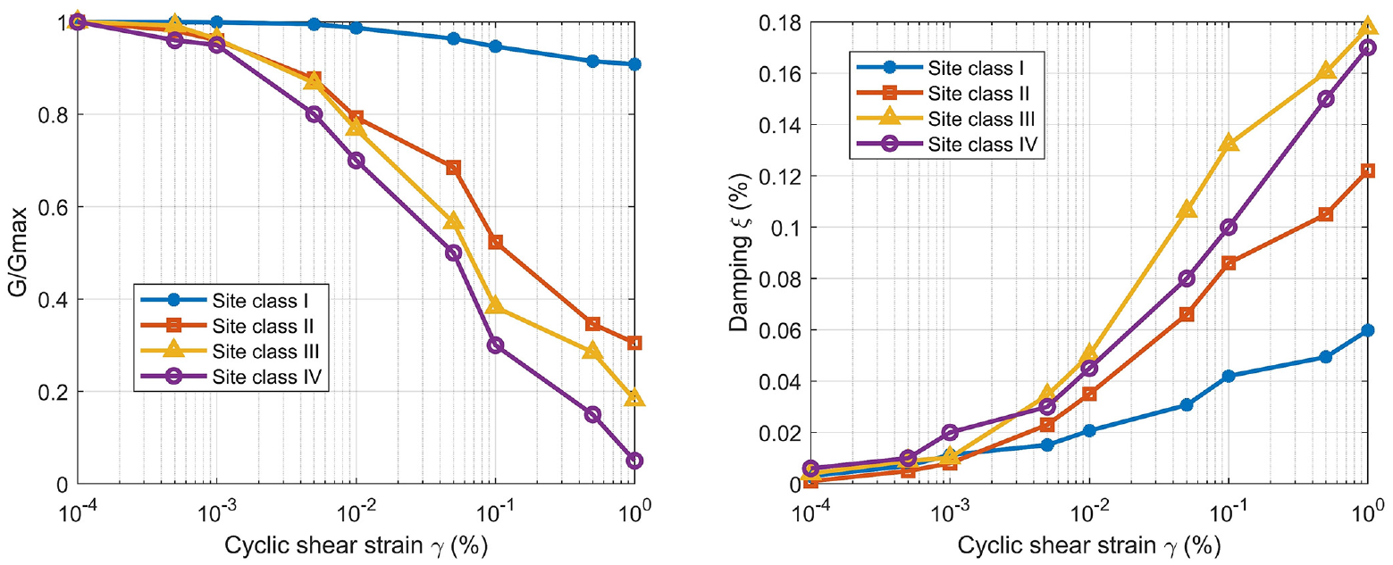
G/G_max and damping curves for site classes I, II, III, and IV.

Shear wave velocity information of surface sedimentary is limited in the Yangbi area, so the V_s30 information, which can be extracted from a global hybrid Vs30 map (Heath et al., 2020) (accessed from USGS website https://earthquake.usgs.gov/data/vs30/), is employed to classify site class. Figure 6 shows the V_s30 distribution map of the Yangbi area. Note that the V_s30 values (unit: m/s) are classified into four ranges as [500, ∞], [250, 500], [150, 250], [0, 150] for site classes I, II, III, and IV, respectively. Procedures to perform the site response correction can be summarized as follows: (1) extract V_s30 information from the global hybrid V_s30 model or other reliable sources like borehole data; (2) determine site class and G/G_max behavior based on V_s30 value; (3) perform equivalent-linear site response analysis with a 30-m-deep homogeneous soil column; (4) repeat the first three steps for all the sites.

Figure 6.

Map of V_s30 (unit: m/s) distribution in Yangbi area. (Extracted from the global hybrid V_s30 model https://earthquake.usgs.gov/data/vs30/).

Ground motion time histories in the two horizontal directions (NS and EW) are simulated up to 20 Hz using the dynamic stiffness matrix method with site response correction. Eight stations including both near-field and far-filed are selected to compare with observed station records. Information of the eight stations is listed in Table 3. Note that the V_s30 and site class information for strong motion stations refers to the work by Xie et al. (2022), which collects borehole data for strong motion stations in Western China. Figure 7 presents the comparison of simulated acceleration time history using the dynamic stiffness matrix method and site response correction with station acceleration records. Duration of the presented time histories is set to be 60 s by removing the zeros before and after the mainshock. Note that the station acceleration records are low-pass filtered with a fourth-order Butterworth filter with low frequency of 0.05 Hz and high frequency of 20 Hz. It is observed that simulated acceleration is in good agreement with station records, especially for the PGA of time histories. However, some discrepancies do exist on waveforms, especially 53BTH and 53LKT stations. It might be due to the topography effects neglected in this study. In addition, Fourier spectra amplitudes of simulated motions are also compared with those of recorded motions, as shown in Figure 8. It is observed that Fourier spectra of simulated motion in the range of 0.1–10 Hz generally agree with recorded motion, and the main discrepancies lie in higher frequencies (>10 Hz). It indicates that although the employed dynamic stiffness method could simulate broadband ground motions, the source model should also be well-calibrated to activate the high-frequency components, especially the source time functions, which are usually not given in source inversion studies.

Table 3.

Information of the selected stations for comparison

Station code	Latitude	Longitude	Distance to epicenter (km)	V_s30 (m/s)	Site class	Recorded PGA (gal)
Station code	Latitude	Longitude	Distance to epicenter (km)	V_s30 (m/s)	Site class	NS	EW	UD
53YBX	25.700	100.000	13.4	655.5	II	339.7	696.1	264.3
53DLY	25.700	100.199	33.1	565.0	II	110.0	88.5	50.1
53YPX	25.500	99.500	41.6	220.0	III	44.2	65.5	79.3
53BTH	25.799	100.500	64.7	760.0	I	6.9	6.4	5.6
53BCJ	25.799	100.599	74.4	565.0	II	22.5	24.7	19.6
53LKT	25.799	98.900	98.3	453.0	II	10.6	10.3	12.8
53SDX	24.700	99.199	127.1	158.8	III	19.0	27.3	9.6
53YRH	26.500	101.000	146.1	369.9	II	6.2	4.4	3.1

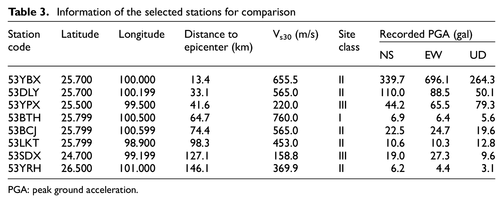
PGA: peak ground acceleration.

Figure 7.

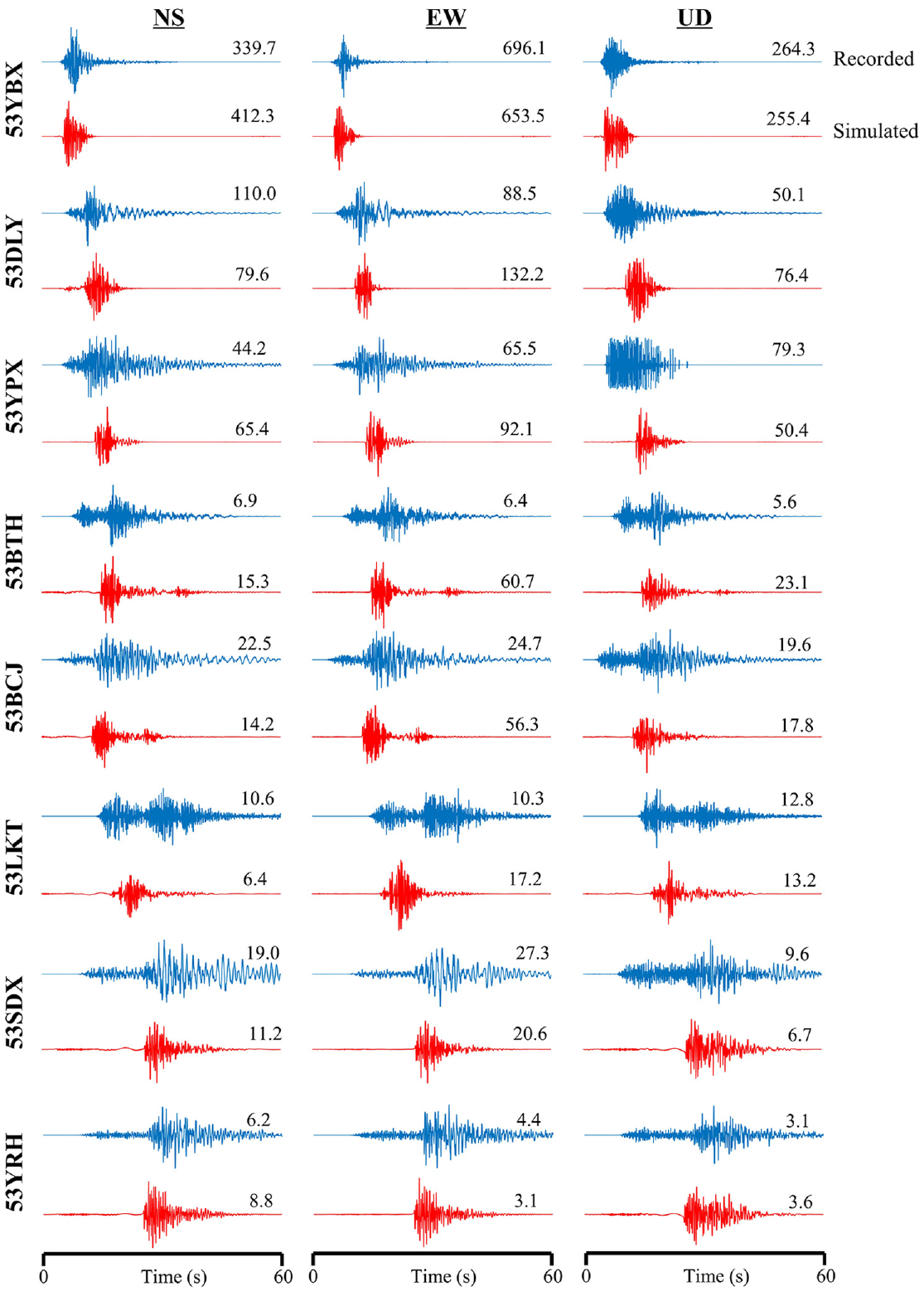
Comparison of simulated acceleration time histories with station records (unit in gal).

Figure 8.

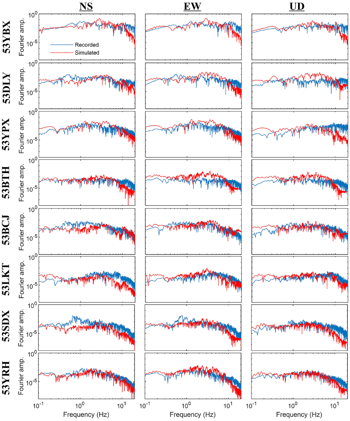
Comparison of Fourier amplitude spectra of simulated acceleration (red color) with station records (blue color).

Figure 9 shows the contour map of PGA of the two horizontal directions. The simulated shaking intensity (PGA) distribution is in general agreement (slight overestimation) with the released observed seismic intensity level contours by the Yunnan Earthquake Agency, China (Li et al., 2023). In addition, the ratio of PGA with site correction to PGA without site correction, also named as “site amplification factor,” is also shown in Figure 10. It is observed that it may significantly impact the intensity of ground motions by taking nonlinear site effect into account. Previous studies reveal that amplification or de-amplification of the site effect is dependent on soil properties, and intensity and frequency content of seismic motion. Furthermore, the distribution of amplification factor in EW direction exhibits the same pattern as that in NS direction, which indicates that, in this study, soil properties play the major role on the amplification effect of site response rather than seismic motion. Figure 11 presents the distribution of site amplification factor for specific site classes I, II, and III. It is observed that the site amplification factor for site class I varies around 1.0 (from 0.9 to 1.1), and site class II exhibits evident amplification with amplification factor ranging from 1.0 to 1.6. Furthermore, site class III presents larger amplification with amplification factor ranging from 1.2 to 1.8. Therefore, the degree of influence on site amplification is “Site class III > Site class II > Site class I.”

Figure 9.

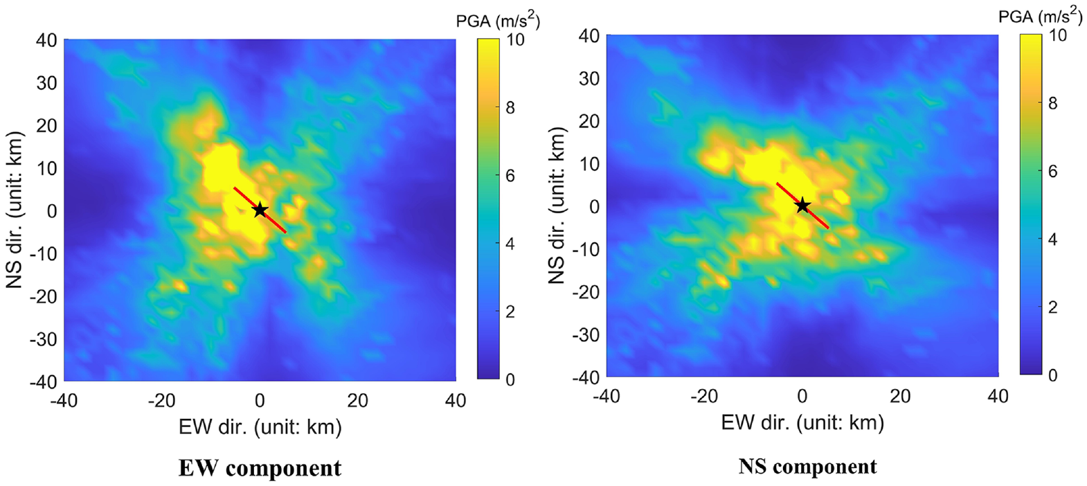
Simulated PGA contour of Yangbi earthquake. (Red line denotes the fault, black star denotes epicenter.)

Figure 10.

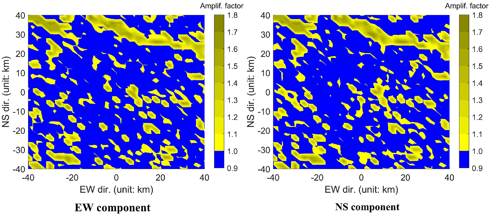
Distribution of site amplification factor (ratio of PGA with site correction to PGA without site correction) for the simulated domain.

Figure 11.

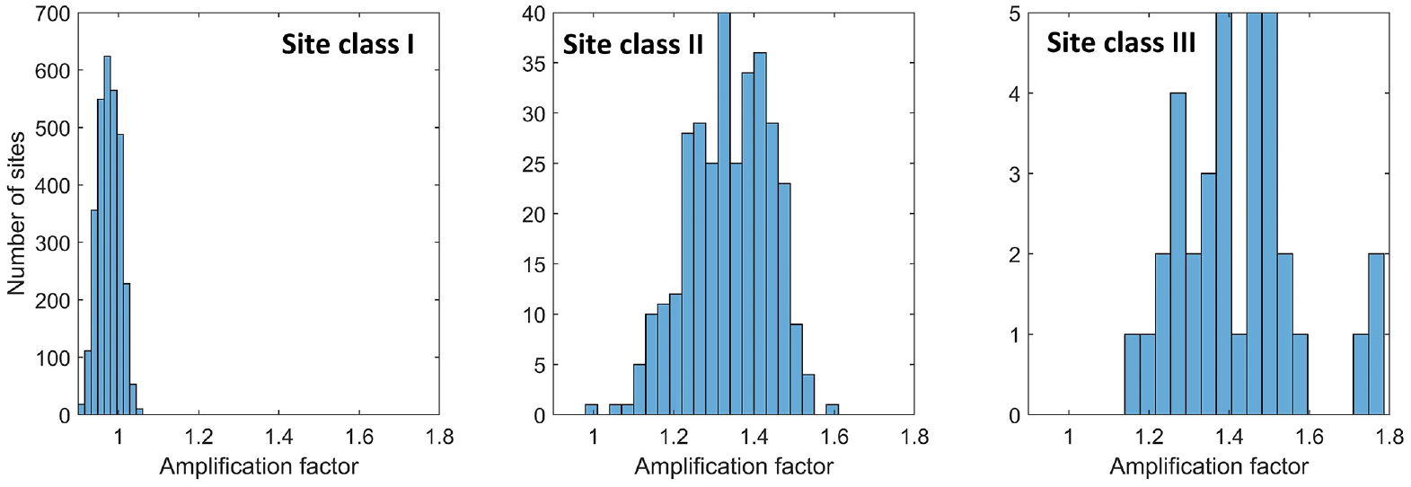
Distribution of site amplification factor for site classes I, II, and III.

Damage estimation for the Yangbi county

Urban area of Yangbi county is around 8 km away on the east of epicenter. By using GIS tools, an inventory of 2216 buildings is established in the urban area of Yangbi county as shown in Figure 12. Note that most of the buildings are low-rise buildings (≤3 stories), and the tallest building is an 8-story building. In addition, with the help of on-site investigation in a limited time, around two-thirds of the buildings are identified as engineered seismic structures (mostly RC frame structures), while the other one-third of the buildings are traditional structures without seismic considerations (mostly traditional wood-adobe structures).

Figure 12.

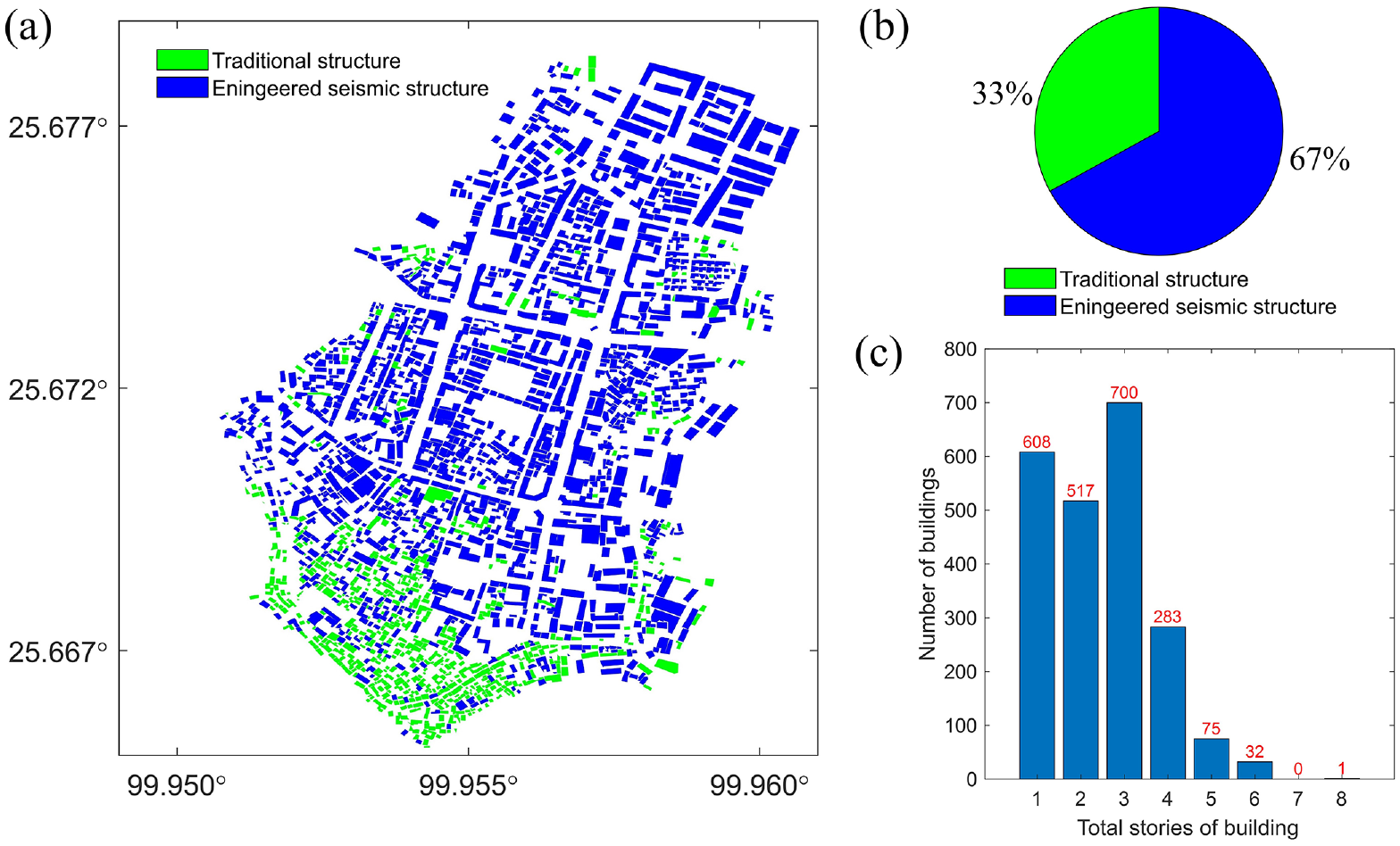
Building information of urban area of Yangbi county: (a) distribution map of buildings with structure type denoted, (b) classification of building’s structure type (traditional structures are mostly wood-adobe structures; Engineered seismic structures are mostly RC frame structures), and (c) distribution of total stories for all buildings.

To estimate the building damage in the urban area of Yangbi county, we employ an urban seismic disaster simulation platform, “YouSimulator”, which was developed by Lin (2017) and Lin et al. (2019), to perform the nonlinear time history analysis for all the buildings and estimate the damage index based on computed building response. It automatically constructs a multi-degree-of-freedom model for the buildings, and computes story mass, stiffness, hysteretic constitutive parameters based on building area, structure type with calibration to account for specific seismic design criteria of the location, and so on. YouSimulator is highly efficient as it can finish nonlinear time history analyses for millions of buildings within 10 min using scalable MPI-based parallel computing.

Building damage is quantified in terms of each story using a damage index ranging from 0 to 1. Figure 13 shows the inter-story nonlinear force-drift model with damage state and damage index identification. As shown in Figure 13a, a trilinear backbone curve is employed as the capacity curve to quantify the damage state. Damage state “Almost None” represents that the story shear force is less than its yield strength; damage states “Minor,”“Moderate,” and “Severe” represent that the story shear force is greater than yield strength but less than strength at collapse point. In addition, the ratio of story drift range for “Minor,”“Moderate,” and “Severe” is defined to be 1:2:3. Damage state “Collapse” represents the story drift past the collapse point. In addition, the story with maximum damage index is selected as the damage index of the whole building. Figure 13b to d shows the hysteretic models for different structure types. As the urban area of Yangbi only has a reinforced concrete frame structure and non-engineered structure, so only the modified Clough model (Mahin and Bertero, 1976) is used in this study.

Figure 13.

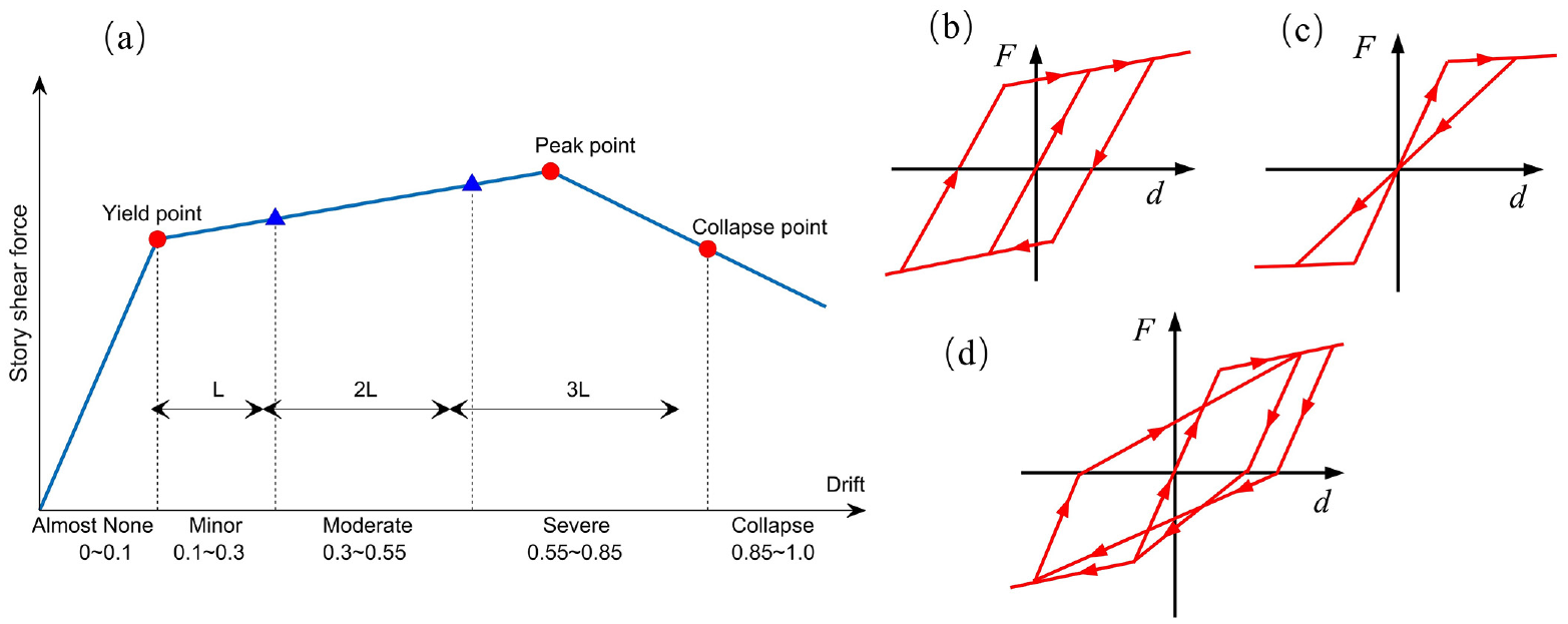
Interstory nonlinear force-drift model with damage state and damage index identification: (a) trilinear backbone curve for all structure types, (b) elastoplastic hysteretic model for steel structure, (c) origin-orientated hysteretic model for timber structure and (d) modified Clough hysteretic model for reinforced concrete, masonry, other non-engineered structures.

As the input ground motion for the urban buildings results from the physics-based Yangbi earthquake simulation and site response correction, spatial variation characteristics are evident, and each building requires its specific input motion. Therefore, YouSimulator is called in a loop to simulate regional buildings response with spatial varying ground motions from physics-based earthquake simulation, which is a highlight in this study and different from the traditional regional analysis using uniform input motion or site-correction-introduced spatial varying motions. Note that the frequency resolution 20 Hz is employed to cover the low-rise building period, especially for single-story buildings with a natural period of less than 0.1 s. Figure 14 presents the simulated results of the time history of relative displacement at the top and inter-story drift ratio of a typical building (Yangbi People’s Hospital Building, RC frame structure) using YouSimulator. The computed damage index is 0.15, which is categorized as a minor damage state. The inter-story drift ratio, close to 0.003, which is larger than the elastic limit of 1/550 but much lower than the elastic-plastic limit of 1/50 in the Chinese seismic design code (MOHURD, 2010), also verifies the damage state estimation as minor damage.

Figure 14.

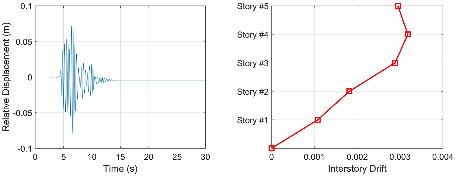
Simulated time history of relative displacement at the top and inter-story drift ratio of a typical building (Yangbi People’s Hospital Building, RC frame structure) using YouSimulator.

Figure 15 shows the distribution of building damage state for all buildings in urban area of Yangbi county. It is observed that nearly all buildings suffered damage, and most buildings suffered minor or moderate damage. In addition, the south part of the buildings is more damaged on average compared to other places, as shown in Figure 15, which is probably due to the south part being the old town and mostly one-story local wood-adobe structures without seismic considerations. Figure 16 presents a statistical analysis of building damage estimation. As observed from the histogram of the damage index for all buildings (Figure 16a), large peaks of the histogram lie in the range of 0.1 and 0.5, which is consistent with the results in Figure 16b that most buildings suffer minor or moderate damage.

Figure 15.

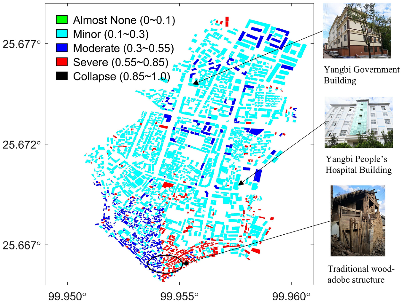
Building damage state distribution of urban area of Yangbi county.

Figure 16.

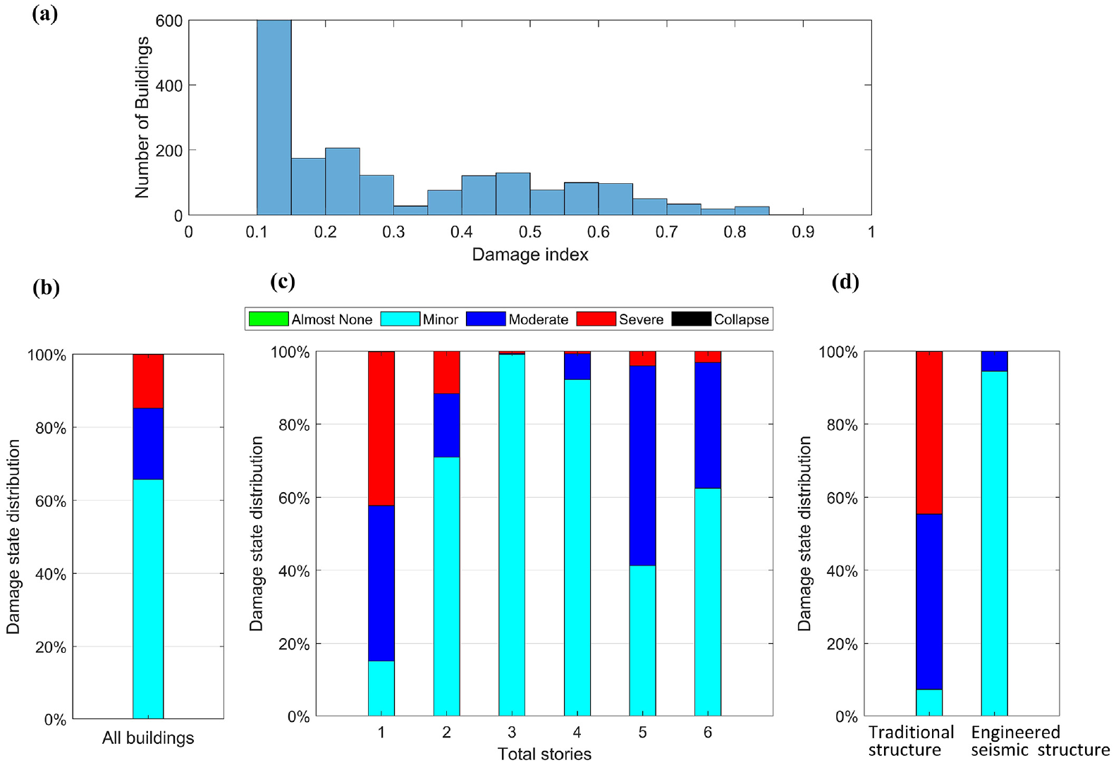
Statistical analysis of building damage estimation for the urban area of Yangbi county: (a) histogram of damage index for all buildings, (b) damage state distribution for all buildings, (c) damage state distribution classified by total stories of buildings and (d) damage state distribution classified by structure type.

Total stories of a building, as a common building property, play a key role in the dynamic characteristics of the structure, which might result in evident amplification and de-amplification in structural response. In addition, it will be more complex with spatial varying ground motions as input for the regional buildings. Figure 16c presents the damage state distribution for buildings with different total number of stories. Results show that one-story structures are mostly moderately or severely damaged, while the other structures are mostly minor damaged or moderately damaged, which generally agrees with field investigation results (Zhang et al., 2021a). In other words, one-story structures are more heavily damaged than other structures, and it is probably due to the fact that one-story structures are mostly local traditional wood-adobe structures without seismic considerations. This observation is also confirmed by the damage state distribution results from Figure 16d, which show that most wood-adobe structures suffer moderate to severe damage, and most engineered seismic structures (RC frame structure) suffer minor damage.

To quantitatively compare with onsite damage observations, we selected two RC frame buildings (Yangbi Government Building and Yangbi People’s Hospital Building) and several traditional wood-adobe structure to validate our damage computations (Li et al., 2021a). Figure 17 shows the typical damage of selected buildings. Typical damage to RC frame buildings includes cracks between infill walls and RC columns, and ceilings fall down. The observed damage of both RC frame buildings could be identified as minor damage, which agree with our estimated damage in Figure 15. On the other hand, selected traditional wood-adobe structures show more evident damage as adobe walls fall down, roof tiles fall off (Figure 17), which agrees with estimated moderate to severe damage in Figures 15 and 16d.

Figure 17.

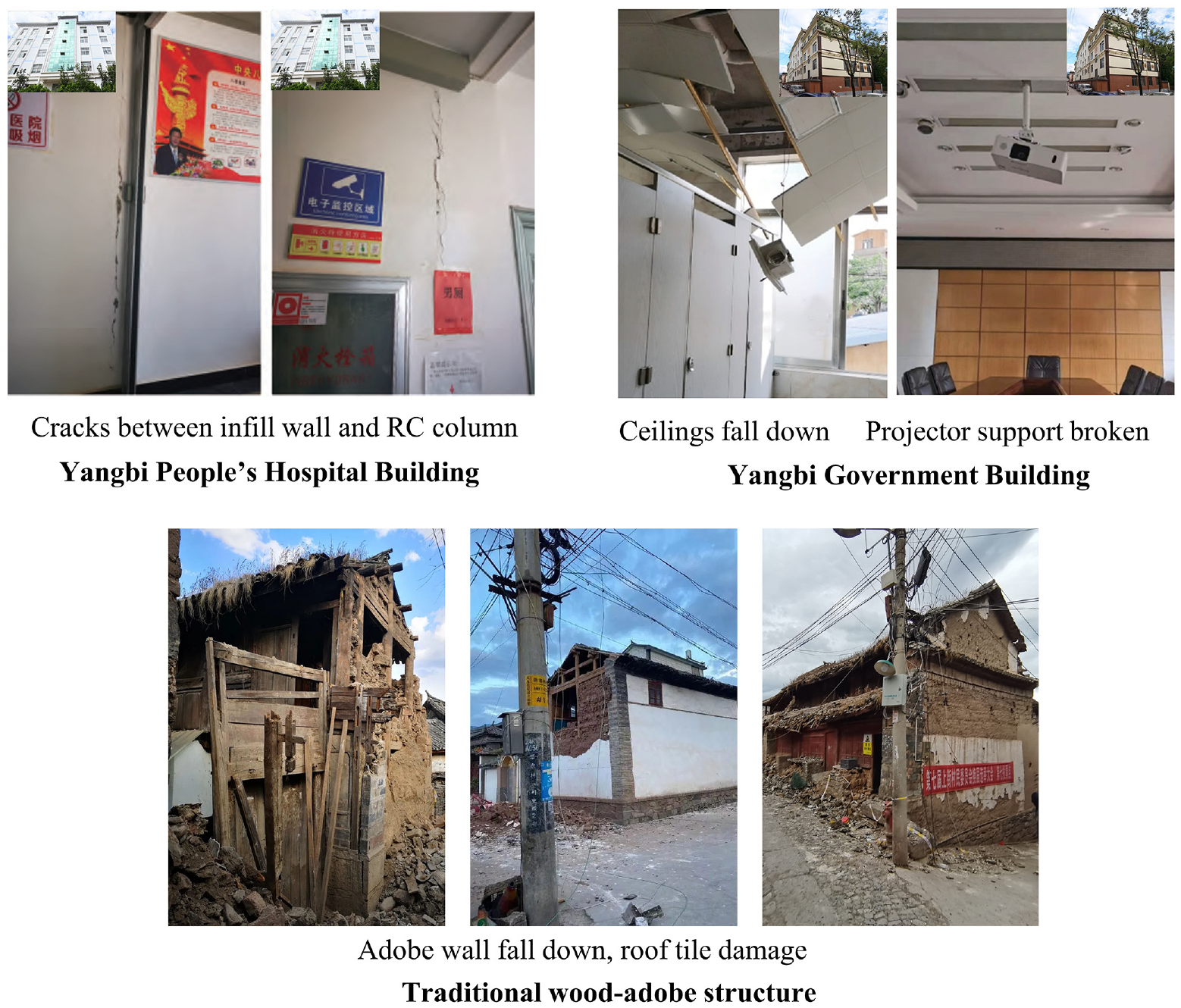
Damage observations for selected typical biuldings: two RC frames and traditional wood-adobe structures.

Conclusion

This article proposes a computational workflow that integrates the efficient dynamic stiffness matrix method in FK domain for physics-based broadband ground motion simulation with city-scale nonlinear time history analysis, to perform seismic damage estimation of buildings in regional urban area. In addition, the ground motions are corrected using equivalent-linear site response analysis. The 2021 M_s 6.4 Yangbi earthquake is simulated and validated through recorded motions, and buildings damage estimation in urban area of Yangbi county is discussed and compared with field observations in this study.

By feeding the simulated ground motions into YouSimulator for nonlinear time history analysis of all buildings, building damage is evaluated based on a trilinear backbone curve of story’s nonlinear force-drift model. Results show that all buildings are identified to be damaged to a certain extent, and most buildings are classified as minor or moderate damage. Especially, one-story buildings suffer more severe damage than other buildings as those are mostly local wood-adobe structures without seismic consideration. Damage estimation results generally agree with field investigation about building damage in Yangbi county. Typical buildings with two RC frames and several traditional wood-adobe structures are selected to quantitatively validate the building damage estimation and prove that specific buildings damage estimation agrees with onsite investigation.

Simulation study of Yangbi county demonstrates that the proposed computational workflow may accurately estimate seismic damage of city-scale buildings under a defined earthquake scenario. It largely relies on the employment of the computational tractable broadband physics-based ground motion simulation, which could capture the intensity and spatial variability of ground motion based on finite fault source, propagation path, and site information. Future work could be fragility analysis and seismic risk assessment of regional buildings based on the proposed computational workflow in this study.

Footnotes

Acknowledgements

Station records provided by the Institute of Engineering Mechanics, China Earthquake Administration are greatly appreciated.

Declaration of conflicting interests

The author(s) declared no potential conflicts of interest with respect to the research, authorship, and/or publication of this article.

Funding

The author(s) disclosed receipt of the following financial support for the research, authorship, and/or publication of this article: The authors are grateful to the financial support of the National Natural Science Foundation of China under grant nos 52108468 and 52178495, Key Laboratory of New Technology for Construction of Cities in Mountain Area under grant no. LNTCCMA-20220111.

ORCID iD

Fangbo Wang

Data and resources

All data and models generated or used during the study appear in the submitted article.

References

Antonietti

Mazzieri

Melas

Paolucci

Quarteroni

Smerzini

Stupazzini

(2021) Three-dimensional physics-based earthquake ground motion simulations for seismic risk assessment in densely populated urban areas. Mathematics in Engineering 3(2): 1–31.

Applied Technology Council (ATC) (1985) Earthquake Damage Evaluation Data for California (ATC-13). Redwood City, CA: ATC.

Liu

Liang

Sang

Zhang

(2022) The dynamic stiffness matrix method for seismograms synthesis for layered transversely isotropic half-space. Applied Mathematical Modelling 104: 205–227.

Sang

Liang

(2021) The revised direct stiffness matrix method for seismogram synthesis due to dislocations: From crustal to geotechnical scale. Geophysical Journal International 227(1): 717–734.

Barbat

Pujades

Lantada

(2008) Seismic damage evaluation in urban areas using the capacity spectrum method: Application to Barcelona. Soil Dynamics and Earthquake Engineering 28(10–11): 851–865.

Campbell

Bozorgnia

(2008) NGA ground motion model for the geometric mean horizontal component of PGA, PGV, PGD and 5% damped linear elastic response spectra for periods ranging from 0.01 to 10 s. Earthquake Spectra 24: 139–172.

Chin

Aki

(1991) Simultaneous study of the source, path, and site effects on strong ground motion during the 1989 Loma Prieta earthquake: A preliminary result on pervasive nonlinear site effects. Bulletin of the Seismological Society of America 81(5): 1859–1884.

Eleftheriadou

Karabinis

(2011) Development of damage probability matrices based on Greek earthquake damage data. Earthquake Engineering and Engineering Vibration 10: 129–141.

Federal Emergency Management Agency (FEMA) (2012) Multi-Hazard Loss Estimation Methodology: HAZUS-MH 2.1—Advanced Engineering Building Module (AEBM) Technical and User’s Manual. Washington, DC: FEMA.

10.

Field

Johnson

Beresnev

Zeng

(1997) Nonlinear ground-motion amplification by sediments during the 1994 Northridge earthquake. Nature 390(6660): 599–602.

11.

Gencturk

Elnashai

(2008) Development and application of an advanced capacity spectrum method. Engineering Structures 30(11): 3345–3354.

12.

Gicev

Trifunac

(2022) High-frequency decay of Fourier spectra of strong motion acceleration and nonlinear site response. Earthquake Engineering and Resilience 1: 302–316.

13.

Graves

Pitarka

(2010) Broadband ground-motion simulation using a hybrid approach. Bulletin of the Seismological Society of America 100(5A): 2095–2123.

14.

Graves

Pitarka

(2015) Refinements to the Graves and Pitarka (2010) broadband ground motion simulation method. Seismological Research Letters 86(1): 75–80.

15.

Haskell

(1953) The dispersion of surface waves on multilayered media. Bulletin of the Seismological Society of America 43: 17–34.

16.

Heath

Wald

Worden

Thompson

Smoczyk

(2020) A global hybrid V_S₃₀ map with a topographic slope–Based default and regional map insets. Earthquake Spectra 36(3): 1570–1584.

17.

Hori

(2006) Introduction to Computational Earthquake Engineering. London: Imperial College Press, 165 pp.

18.

Hori

Ichimura

(2008) Current state of integrated earthquake simulation for earthquake hazard and disaster. Journal of Seismology 12(2): 307–321.

19.

Idriss

Sun

(1993) User’s Manual for Shake91: A Computer Program for Conducting Equivalent Linear Seismic Response Analyses of Horizontally Layered Soil Deposits. Davis, CA: Center for Geotechnical Modeling, Department of Civil and Environmental Engineering, University of California, Davis.

20.

Jayaram

Baker

(2009) Correlation model for spatially distributed ground-motion intensities. Earthquake Engineering & Structural Dynamics 38(15): 1687–1708.

21.

Jiang

Tao

Cao

Wang

(2021) Scaling laws of local parameters of finite fault source model. Earthquake Engineering and Engineering Vibration 37(6): 23–30 (in Chinese).

22.

Kausel

Roesset

(1977) Semianalytic hyperelement for layered strata. Journal of the Engineering Mechanics Division 103(4): 569–588.

23.

Kenawy

McCallen

Pitarka

(2021) Variability of near-fault seismic risk to reinforced concrete buildings based on high-resolution physics-based ground motion simulations. Earthquake Engineering & Structural Dynamics 50(6): 1713–1733.

24.

Knopoff

(1964) A matrix method for elastic wave problems. Bulletin of the Seismological Society of America 54: 431–438.

25.

Zhou

Tao

(2021a) Seismic damage to public buildings in the M6.4 Yangbi earthquake in Yunnan. World Earthquake Engineering 37(3): 1–8 (in Chinese).

26.

Sun

Rong

Zhang

Wang

(2023) Characteristics of building seismic damages in M_s6.4 Yangbi Earthquake affected by ground motion directivity and site condition. Journal of Basic Science and Engineering 31(3): 650–662 (in Chinese).

27.

Jin

Miao

(2021b) Relocation of the 2021 Yangbi, slip model and co-seismic displacement field of the 2021 Yangbi, Yunnan M_s 6.4 earthquake. Journal of Seismological Research 44(3): 330–337.

28.

Liang

(2007) Exact dynamics stiffness matrices of 3-D layered site and its Green’s functions. Earthquake Engineering and Engineering Vibration 27(5): 7–17 (in Chinese).

29.

Lin

(2017) Earthquake disaster simulations and risk control for city buildings. City and Disaster Reduction 3: 18–22.

30.

Lin

Wang

Zhang

Skalomenos

(2019) Development of a simulation platform to model, assess and visualize the earthquake disasters in city level. In: Proceedings of the 2nd international conference on natural hazards and infrastructure, Chania, 23–26 June.

31.

Cheng

Sun

(2019) Real-time city-scale time-history analysis and its application in resilience-oriented earthquake emergency responses. Applied Sciences 9(17): 3497.

32.

McKenna

Cheng

Zeng

Mahin

(2020) An open-source framework for regional earthquake loss estimation using the city-scale nonlinear time history analysis. Earthquake Spectra 36(2): 806–831.

33.

McCallen

Petersson

Rodgers

Pitarka

Miah

Petrone

Sjogreen

Abrahamson

Tang

(2021) EQSIM—A multidisciplinary framework for fault-to-structure earthquake simulations on exascale computers Part I: Computational models and workflow. Earthquake Spectra 37: 707–735.

34.

Mahin

Bertero

(1976) Nonlinear seismic response of a coupled wall system. Journal of the Structural Division: ASCE 102(9): 1759–1780.

35.

Mai

Imperatori

Olsen

(2010) Hybrid broadband ground-motion simulations: Combining long-period deterministic synthetics with high-frequency multiple S-to-S backscattering. Bulletin of the Seismological Society of America 100(5A): 2124–2142.

36.

Mimura

Yasuhara

Kawagoe

Yokoki

Kazama

(2011) Damage from the Great East Japan Earthquake and tsunami—A quick report. Mitigation and Adaptation Strategies for Global Change 16: 803–818.

37.

Ministry of Housing and Urban-Rural Development of the People’s Republic of China (MOHURD) (2010) Code for Seismic Design of Buildings (GB 50011-2010). Beijing, China: Building Industry Press of China (in Chinese).

38.

Nettis

Gentile

Raffaele

Uva

Galasso

(2021) Cloud Capacity Spectrum Method: Accounting for record-to-record variability in fragility analysis using nonlinear static procedures. Soil Dynamics and Earthquake Engineering 150: 106829.

39.

Norton

King

Bull

Chapman

McVerry

Larkin

Spring

(1994) Northridge earthquake reconnaissance report. Bulletin of the New Zealand Society for Earthquake Engineering 27(4): 235–344.

40.

Paolucci

Gatti

Infantino

Smerzini

Özcebe

Stupazzini

(2018) Broadband ground motions from 3D physics-based numerical simulations using artificial neural networks. Bulletin of the Seismological Society of America 108(3A): 1272–1286.

41.

Peter

Badoux

(2000) Application of the capacity spectrum method to RC buildings with bearing walls. In: Proceedings of the 12th world conference on earthquake engineering, Auckland, New Zealand, 30 January–4 February.

42.

Pitarka

Thio

Somerville

Bonilla

(2013) Broadband ground-motion simulation of an intraslab earthquake and nonlinear site response: 2010 Ferndale, California, earthquake case study. Seismological Research Letters 84(5): 785–795.

43.

Rong

Wang

Sheng

Huang

Fang

(2013) Calculation and analysis of seismic ground motion parameters for different engineering geological divisions of Chengdu Basin. Acta Seismologica Sinica 35(4): 543–552.

44.

Seylabi

Restrepo

Taborda

Asimaki

(2021) Deterministic ground motion simulations with shallow crust nonlinearity at Garner Valley in Southern California. Earthquake Engineering & Structural Dynamics 50(1): 43–59.

45.

Smerzini

Pitilakis

(2018) Seismic risk assessment at urban scale from 3D physics-based numerical modeling: The case of Thessaloniki. Bulletin of Earthquake Engineering 16(7): 2609–2631.

46.

Taborda

Bielak

Restrepo

(2012) Earthquake ground-motion simulation including nonlinear soil effects under idealized conditions with application to two case studies. Seismological Research Letters 83(6): 1047–1060.

47.

Thomson

(1950) Transmission of elastic waves through a stratified solid medium. Journal of Applied Physics 21: 89–93.

48.

Wang

Shen

Xie

Weng

(2023) Ground motion simulation for the 21 May 2021 M_s 6.4 Yangbi, China, earthquake using stochastic finite-fault method. Earthquake Spectra 39(1): 528–550.

49.

Wang

Zhou

Hao

Zhao

Yao

(2022) Rupture process models of the Yangbi and Maduo earthquakes that struck the eastern Tibetan Plateau in May 2021. Science Bulletin 67: 466–469.

50.

Wolf

(1985) Dynamic Soil-Structure Interaction. Englewood Cliffs, NJ: Prentice Hall.

51.

Xie

Wen

Jia

Cui

Lin

Zhang

Jiang

Xie

Wang

Zimmaro

Stewart

(2022) Soil profile database and site classification for national strong-motion stations in Western China. Seismological Research Letters 93(3): 1930–1942.

52.

Xiong

Lin

(2017) Parameter determination and damage assessment for THA-based regional seismic damage prediction of multi-story buildings. Journal of Earthquake Engineering 21(3): 461–485.

53.

Zeng

Wang

(2013) Wenchuan, China (2008 earthquake). In: Bobrowsky

(ed.) Encyclopedia of Natural Hazards (Encyclopedia of earth sciences series). Dordrecht: Springer, pp. 1097–1102.

54.

Zhang

X-J

Rong

M-S

Wang

(2021a) Analysis of strong ground motion characteristics and earthquake damage for the Yangbi M_s 6.4 earthquake, Yunnan. Seismology and Geology 43(5): 1127–1139 (in Chinese).

55.

Zhang

Mavroeidis

Wang

Papageorgiou

(2022) Validation of physics-based regional-scale ground-motion simulations of the 2008 M_w 7.9 Wenchuan earthquake for engineering applications. Earthquake Engineering & Structural Dynamics 51(12): 2975–2999.

56.

Zhang

Chen

Crempien

JGF

Kurtulus

Arduino

Taciroglu

(2023a) Regional-scale seismic fragility, loss, and resilience assessment using physics-based simulated ground motions: An application to Istanbul. Earthquake Engineering & Structural Dynamics 52: 1785–1804.

57.

Zhang

Crempien

JGF

Kurtulus

Chen

P-Y

Arduino

Taciroglu

(2023b) A suite of broadband physics-based ground motion simulations for the Istanbul region. Earthquake Engineering & Structural Dynamics 52: 1161–1181.

58.

Zhang

Restrepo

Crempien

JGF

Erkmen

Taborda

Kurtulus

Taciroglu

(2021b) A computational workflow for rupture-to-structural-response simulation and its application to Istanbul. Earthquake Engineering & Structural Dynamics 50: 177–196.

59.

Zhu

Luo

Zhao

Tian

(2022) Rupture process of Yunnan Yangbi M_s6.4 earthquake constrained by regional broadband seismograms. Chinese Journal of Geophysics 65(3): 1021–1031 (in Chinese).

City-scale buildings damage estimation based on broadband physics-based ground motion simulation of 2021 M s 6.4 Yangbi,China,earthquake

Abstract

Keywords

Introduction

Broadband ground motion simulations of 2021 Ms 6.4 Yangbi earthquake

Establishment of the hybrid kinematic fault model

Earthquake simulations using dynamic stiffness matrix method

Site response correction

Damage estimation for the Yangbi county

Conclusion

Footnotes

Acknowledgements

Declaration of conflicting interests

Funding

ORCID iD

Data and resources

References

Broadband ground motion simulations of 2021 M_s 6.4 Yangbi earthquake