Subsurface imaging dataset acquired at the Garner Valley Downhole Array site using a dense network of three-component nodal stations

Abstract

There is a growing need to characterize the engineering material properties of the shallow subsurface in three dimensions for advanced engineering analyses. However, imaging the near-surface in three dimensions at spatial resolutions required for such purposes remains in its infancy and requires further study before it can be adopted into practice. To enable and accelerate research in this area, we present a large subsurface imaging data set acquired using a dense network of three-component (3C) nodal stations acquired in 2019 at the Garner Valley Downhole Array (GVDA) site. Acquisition of this data set involved the deployment of 196 stations positioned on a 14 × 14 grid with a 5 m spacing. The array was used to acquire active-source data generated by a vibroseis truck and an instrumented sledgehammer, and passive-wavefield data containing ambient noise. The active-source acquisition included 66 vibroseis and 209 instrumented sledgehammer source locations. Multiple source impacts were recorded at each source location to enable stacking of the recorded signals. The active-source recordings are provided in terms of both raw, uncorrected units of counts and corrected engineering units of meters per second. For each source impact, the force output from the vibroseis or instrumented sledgehammer was recorded and is provided in both raw counts and engineering units of kilonewtons. The passive-wavefield data include 28 h of ambient noise recorded over two nighttime deployments. The data set is shown to be useful for active-source and passive-wavefield three-dimensional imaging and other subsurface characterization techniques, which include horizontal-to-vertical spectral ratios (HVSRs), multichannel analysis of surface waves (MASW), and microtremor array measurements (MAM).

Introduction

The ability to reliably and non-invasively measure engineering material properties of three-dimensional (3D) subsurface volumes at high spatial resolution has the potential to revolutionize site characterization. While work has been ongoing in this area over the past several years (e.g. Fathi et al., 2016; Tran et al., 2019), progress toward a practical 3D imaging approach that can be applied routinely for engineering analyses remains out of reach. The authors believe that this is due in part to the lack of publicly available, high-quality, large-scale field data sets for near-surface 3D imaging in locations of engineering interest. As evidence for this, new geophysical methods (e.g. Butzer et al., 2013; Wang et al., 2019) are often applied only on synthetic data due to the lack of high-quality field data sets and invasive data for verification. In response, this work presents a high-quality, large-scale field data set for near-surface 3D imaging acquired at the Garner Valley Downhole Array (GVDA) site in southern California.

Site overview

The GVDA is located in southern California approximately 70 miles northeast of San Diego and 90 miles southeast of Los Angeles. The GVDA exists in a seismically active region 7 km from the San Jacinto Fault and 35 km from the San Andreas Fault. Instrumentation at the GVDA began in 1989 and includes multiple ground-motion recording stations at the surface and at depth (Archuleta et al., 1992). The site is particularly interesting from an earthquake engineering perspective, as quite a few previous studies (Afshari and Stewart, 2019; Bonilla et al., 2002; Steidl et al., 1996; Tao and Rathje, 2019; Teague et al., 2018; Vantassel and Cox, 2019) have attempted to match the frequency-dependent site amplifications observed at the GVDA using one-dimensional (1D) ground response analyses (GRAs), but with rather limited success. In fact, this has led several authors to hypothesize that the GVDA site amplification is significantly influenced by non-1D behaviors. As such, this makes the GVDA site an interesting test bed for 3D site characterization efforts.

A plan view of the GVDA site is shown in Figure 1. Stars denote three of the site’s permanent ground-motion accelerometers; 00 and 08 at the surface (i.e. 0 m depth), and 05 located at 150 m depth. The GVDA site has been the focus of a number of previous invasive site characterization efforts. Of those efforts, two were performed to sufficient depth to be of interest for GRA-type analyses: the PS suspension logging performed by Steller (1996) and the downhole test performed by Gibbs (1989). The location of the PS suspension logging is known fairly accurately (within a few meters) and is shown with a pentagon in Figure 1. The location of the downhole test, however, is not well known. Its approximate position was estimated from a map provided in the report by Gibbs (1989) and is shown in Figure 1 with a triangle, although the true location may be anywhere within a 30 m radius of the location indicated.

Figure 1.

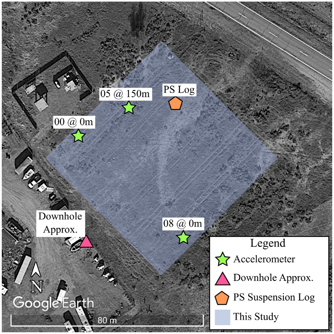
Plan view of the GVDA site with the locations of three of the permanent ground-motion accelerometers indicated with stars, the approximate location of the seismic downhole test performed by Gibbs (1989) indicated with a triangle, the location of the PS suspension logging performed by Steller (1996) indicated with a pentagon, and the shaded area indicating the region of interest for the present study.

Several previous non-invasive site characterization efforts have also been conducted at the GVDA site. These include spectral analysis of surface wave (SASW) tests performed by Stokoe et al. (2004), a 3D full waveform inversion (FWI) data set collected with 1C geophones reported by Fathi et al. (2016), and multichannel analysis of surface waves (MASW) and microtremor array measurement (MAM) tests documented by Teague et al. (2018). Of these efforts, only the data reported by Fathi et al. have been openly published (Bielak et al., 2012), and while it is an early and extremely valuable data set for active-source FWI studies, it is significantly less expansive than the present data set in terms of the number of receivers, receiver components, number and type of active-sources, and inclusion of passive-wavefield data. As the array and receiver locations used for these studies are too numerous to show in Figure 1, we refer the reader to the publications noted above for detailed descriptions of the experimental layouts relative to the GVDA site’s instrumentation.

Site geology

The geology of the GVDA site includes three primary geologic layers: alluvial sediments (AL), decomposed granite (DG), and competent granite (GR) (Archuleta et al., 1992). The AL contains a mixture of silty sand, clayey sand, and silty gravel (Archuleta et al., 1992; Youd et al., 2004). Lake Hemet, the result of the Hemet Dam whose shoreline is located approximately 500 m to the west of the downhole array (Hill, 1981), serves to maintain a groundwater table between 1 and 3 m (Steidl et al., 1996), with some having measured it as deep as 5 m (Gibbs, 1989). The bottom depth of the AL has been estimated using a variety of geotechnical and geophysical techniques. These tests include downhole testing by Gibbs (1989), which estimated the bottom of the AL at approximately 18 m; standard penetration testing (SPT) performed by Pecker and Mohammadioun (1991), which also estimated the bottom of AL at about 18 m; PS suspension logging performed by Steller (1996), which estimated a gradual transition between the AL and DG between 10 and 20 m; and spectral analysis of surface waves testing performed by Stokoe et al. (2004), which estimated the transition at approximately 24 m. In addition, cone penetration tests (CPTs) performed by Youd et al. (2004) estimated the bottom of the AL deposit to range from 18 to 25 m across the site. Most recently, MASW and MAM by Teague et al. (2018) estimated the thickness of the AL between 15 and 20 m. The range of estimates of the AL’s thickness seems to imply that the interface between the AL and the DG at GVDA may vary across the site, hinting at non-1D site conditions. Underlying the AL is the DG. The estimated bottom depth of the DG, much like the AL deposits, varies between sources. Gibbs (1989) estimated the depth to GR as approximately 65 m; Archuleta et al. (1992), who reinterpreted the data from Gibbs (1989), estimated it between 40 and 45 m; Steller (1996) estimated it at approximately 87 m; and Teague et al. (2018) estimated it between 40 and 70 m. The potential for high variability in AL and DG layers at the site prompted the acquisition of the high-quality, large-scale imaging data set whose presentation and documentation is the primary focus of this work.

Overview of the data set

The data set documented in this work was collected at the GVDA site between October 6 and October 10, 2019. It involved the deployment of 196 three-component (3C) stations borrowed from IRIS PASSCAL. As shown in Figure 1, the array encompassed the spatial location of the PS suspension logging by Steller (1996) and the three aforementioned permanent seismic accelerometers, and was as close as possible to the approximate location of the downhole testing by Gibbs (1989). The array was used to record both active-source and passive-wavefield data. The former includes 209 source locations with an instrumented sledgehammer and 66 source locations with a vibroseis, whereas the latter includes 28 h of ambient noise. All of the data discussed in this work have been archived and made publicly available through DesignSafe-CI (Rathje et al., 2017) under the project titled, “Active-Source and Passive-Wavefield Nodal Station Measurements at the Garner Valley Downhole Array” (Vantassel et al., 2023).

Instrumentation

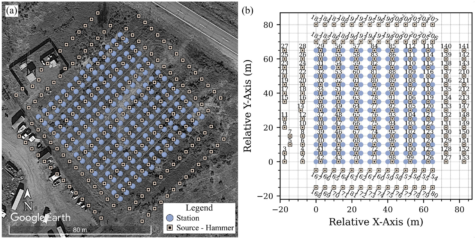
The 196 nodal stations were arranged at the site in a 14 × 14 grid at a 5 m spacing, as shown in Figure 2a. The square array was oriented approximately 45° clockwise from north to allow it to include the ground-motion accelerometers and PS suspension logging test location, and to avoid as much as possible on-the-ground obstructions. The first step of installing the array was to establish a relative coordinate system. The array’s western-most corner was selected as relative coordinate (0, 0), with positive x-values pointing to the southeast and positive y-values to the northeast. The x–y arrows in Figure 2a denote the orientation of the array’s relative coordinate system, with the layout of the array on that relative coordinate system shown in Figure 2b. Each line of the square array is denoted with a four-character designation, with the first two characters denoting its orientation (NS or EW) and the second two its position from the array’s western-most corner (00 to 13). In Figure 2b, the sequential array position numbers of select stations are indicated directly above their corresponding circle symbol. These sequential array position numbers are used to designate each station in the published data set. The location of all stations was positioned in the field using a total station. Note that the surveying process was non-trivial due to the aforementioned obstructions and significant plant life at the site. A picture of the surveying process is shown in Figure 3a. Note the knee-high grass and other larger plant life in the photo’s background. It took approximately 10 h to survey all 196 stations to an accuracy of 5 cm. The as-built locations of all stations, including those that needed to be moved to avoid obstructions, are provided as part of the data set in both relative (i.e. x–y) and absolute coordinates (i.e. latitude–longitude). Figure 2a and b show the as-built locations of all stations.

Figure 2.

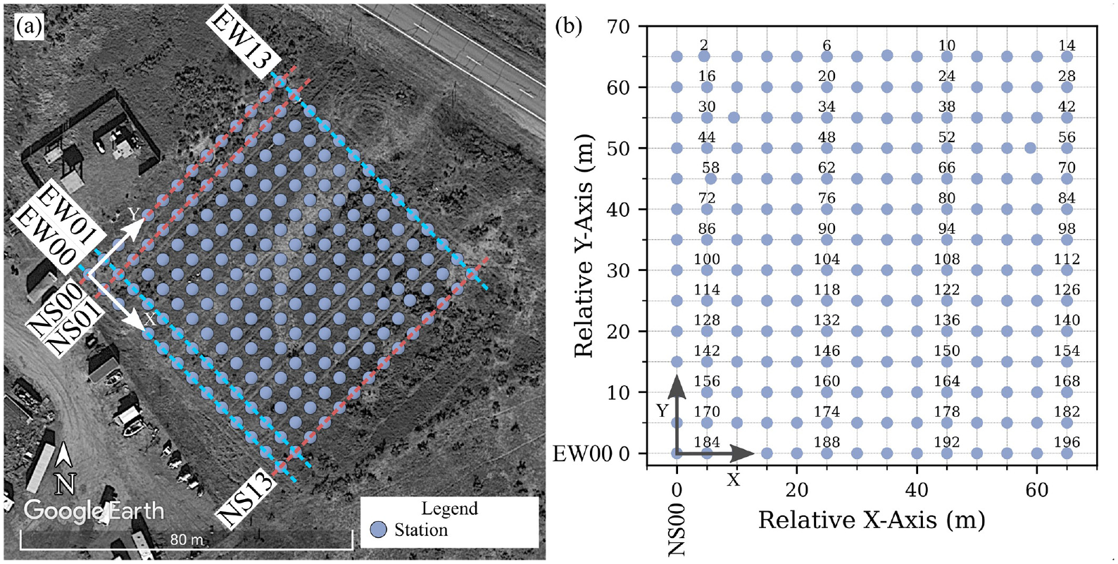
Panel (a) shows the as-built location of all 196, 3C nodal stations deployed at the GVDA site. Each line of the square array is denoted with a four-character designation, with the first two characters denoting its orientation (NS or EW) and the second two its position from the array’s western-most corner (00 to 13). Panel (b) shows the as-built array on its relative coordinate system with the sequential array position numbers of select stations indicated directly above their corresponding circle symbol. The orientation of the relative coordinate system shown in panel (b) is indicated with x–y arrows in panel (a).

Figure 3.

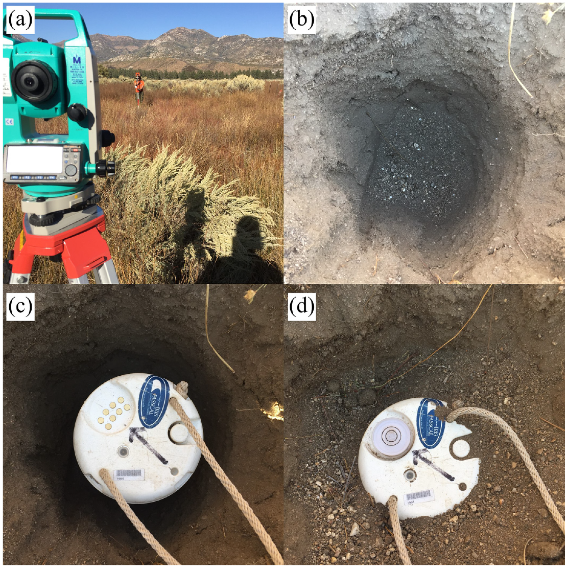
The 3C nodal station installation process involved: (a) surveying each position to within a 5 cm accuracy using a total station, (b) excavating a hole for each station approximately 18 cm deep and 15 cm in diameter, (c) placing the sensor in the hole and orienting it to magnetic north, and (d) backfilling and leveling the senor.

Following the layout of the array, holes (approximately 18 cm deep and 15 cm in diameter) were excavated to bury the nodal stations. A picture of a typical hole is shown in Figure 3b. Notably, the near-surface materials at the GVDA site were highly variable, ranging from easy-to-excavate clean sand to hard-to-excavate heavily cemented material. The 3C stations were placed into the excavated holes, oriented to magnetic north (see Figure 3c), leveled, and backfilled (see Figure 3d). Because the nodal stations were buried, the large central spike attached to the base of each nodal station was removed to accelerate installation. The process of installing and activating the stations took a crew of five approximately 5.5 h to complete (3.5 h to install and 2 h to activate).

The nodal stations deployed at GVDA were Fairfield Nodal ZLand 3C equipped with three orthogonal 5 Hz geophones (two horizontal and one vertical), an internal battery, and a GPS time-synced digitizer with an accuracy of ± 10 μs. The nodal stations were borrowed from the PASSCAL Instrumentation Center as part of the project, “Data Acquisition for 2020 Blind Trial of Surface-based Site Characterization Methods” led by Alan Yong (2019). For their deployment at GVDA, the stations were configured with a passive mode setup that included a 24 dB gain and 2000 Hz sampling rate (0.5 ms time step). The stations were left to record continuously in passive mode through the duration of the experiment, including during active-source data acquisition. The decision to leave the stations in a passive mode configuration, rather than switching them between two configurations (one for active with a low or zero gain and one for passive with a higher gain), was done as a matter of convenience in the field, as each switch between modes would have required at least 2 h. Leaving the stations in the passive mode configuration allowed more time for active-source data acquisition, while, as discussed in detail later, only moderately complicating post-acquisition processing. In hindsight, the authors believe trading post-processing complexity for faster field acquisition was worthwhile, as it allowed the acquisition of more data in the limited time available. Importantly, the authors have seen no evidence that the choice to use a pure passive mode deployment had any negative effect on the final data quality.

Active-source data acquisition

Active-source data acquisition was first performed using a vibroseis source. The vibroseis source used in this study was the highly mobile shaker truck Thumper from the NHERI@UTexas experimental facility (Stokoe et al., 2020). Thumper was used to shake in the vertical direction with a linear frequency sweep from 5 to 30 Hz over a 12-s duration. Thumper was run in high-force-output mode, which at the GVDA site was able to reliably produce approximately 30 kilonewtons (kN) of ground force. During shaking, a Nanometrics’ Centaur digitizer was connected directly to Thumper’s electronics (i.e. into vibeout) to record the force output at a sampling rate of 2000 Hz (0.5 ms time step). Using a digitizer such as the Nanometrics’ Centaur that is GPS time-synchronizer was imperative to ensure a reliable point of reference between the source and the nodal stations, as no time break or seismic event recorder was used in the field to “trigger” data acquisition on the stations. Therefore, extracting records for individual source events had to be done as part of post-acquisition processing and will be discussed in detail later. As shown in Figure 4a, Thumper was used to shake at 41 locations inside the array (i.e. interior source locations) and 25 locations outside of the array (i.e. exterior source locations) (66 in total). Coordinates for all Thumper shaking locations are tabulated in the published data set. Note that it was not possible to test along the array’s northwestern and southeastern edges and at some locations to the north due to the presence of fencing and construction debris. Figure 4b shows the vibroseis source locations with their numeric identifier relative to the nodal stations on the site’s relative coordinate system. Note that the vibroseis source numbers are not sequential, with some numbers missing. Missing numbers correspond to other source locations used in the field but not related to the data set presented here. At each source location three identical shakes were performed to allow subsequent stacking of the measured signals.

Figure 4.

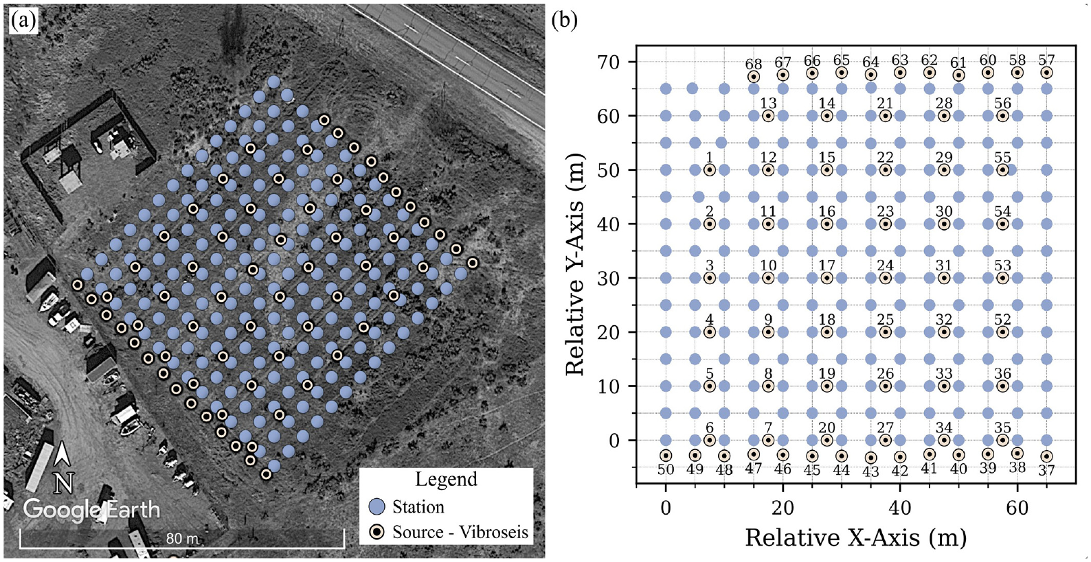
Panel (a) shows a plan view of the GVDA site with the 66 (41 interior; 25 exterior) vibroseis source locations relative to the 196 nodal stations. Note that it was not possible to operate the vibroseis along the array’s northwestern and southeastern edges due to the presence of fencing and construction debris. Some other regularly spaced source locations also had to be skipped due to access restrictions. Panel (b) shows the vibroseis source locations with their numeric identifiers relative to the nodal stations on the site’s relative coordinate system. Note that the vibroseis source numbers are not sequential, with some numbers missing. Missing numbers correspond to other source locations used in the field but not related to the data set presented here.

Following the vibroseis data acquisition, the sledgehammer source was used. The sledgehammer used in this study was a 5.4 kg instrumented sledgehammer from PCB Piezotronics. At each hammer source location, the hammer was swung vertically against an aluminum strike plate. A Nanometrics’ Centaur digitizer was used to record the signal from the instrumented sledgehammer’s load cell with a sampling rate of 2000 Hz (0.5 ms time step). The force output and frequency content from the instrumented sledgehammer varied with the operator and the ground conditions, but on average at the GVDA site, the sledgehammer produced a peak force output of approximately 20 kN. As shown in Figure 5a, the sledgehammer source was used at 98 interior source locations and at 111 exterior shot locations (209 in total). Note that the source locations on the western side of the array had to be adjusted from their planned locations and in one case, canceled to avoid equipment associated with the GVDA. Figure 5b shows the hammer source locations with their numeric identifier relative to the nodal stations on the site’s relative coordinate system. As with the vibroseis source numbers, the hammer source numbers are not sequential with some numbers missing. Missing numbers correspond to other source locations used in the field but not related to the data set presented here. Coordinates for all of the hammer source locations are tabulated in the published data set. At each location, at least five source impacts were performed to allow subsequent stacking of the measured signals.

Figure 5.

Panel (a) shows a plan view of the GVDA site with the 209 (98 interior; 111 exterior) hammer source locations relative to the 196 nodal stations. Note that the source locations on the northwestern side of the array had to be adjusted from their planned locations and, in one case, canceled altogether to avoid equipment associated with the GVDA. Panel (b) shows the hammer source locations with their numeric identifiers relative to the nodal stations on the site’s relative coordinate system. Note that the hammer source numbers are not sequential, with some numbers missing. Missing numbers correspond to other source locations used in the field but not related to the data set presented here.

Post-acquisition processing

At the conclusion of data acquisition, the stations were deactivated, excavated, cleaned, and packaged for shipment back to IRIS PASSCAL. Once the stations were received by IRIS PASSCAL, the data were downloaded, archived on the IRIS Data Management Center (DMC), and provided to the project team. As all of the data for the GVDA experiment were recorded in a passive mode configuration, there were two main post-acquisition processing tasks: (1) downloading, post-processing, and organizing the passive-wavefield data in an easy-to-reuse format and (2) identifying when each active-source event occurred using the source recordings, extracting the corresponding receiver data from the IRIS DMC, and providing the extracted events in an easy-to-reuse format.

The first and easier of the two tasks was to download and post-process the passive-wavefield data. There were two passive-wavefield recording periods. The first was a 15-h block from 18:00 Pacific Daylight Time (PDT) on October 8, 2019 to 09:00 PDT on October 9, 2019, and the second was a 13-h block from 19:00 PDT on October 9, 2019 to 08:00 PDT on October 10, 2019. Following standard practice, the passive-wavefield data in our data set are archived in coordinated universal time (UTC), not PDT, and therefore, the aforementioned blocks correspond to 01:00 UTC to 16:00 UTC on October 9, 2019 and 02:00 UTC to 15:00 UTC on October 10, 2019, respectively. For archiving the passive-wavefield data on DesignSafe, two formats were under consideration: comma-separated value (CSV) and miniSEED (a subset of the Standard for the Exchange of Earthquake Data (SEED) format). Ultimately, it was decided that the miniSEED format would allow for the greatest ease-of-reuse, as most ambient-noise-focused geophysical software accepts miniSEED as input, and there also exists several open-source libraries to read miniSEED (e.g. obspy, libmseed) for writing the data into other formats. In addition, using a binary-based format such as miniSEED (rather than a text-based format, such as CSV) minimizes the disk space required to hold the data. To enable users to easily access subsets of the data, one miniSEED file was saved per station (i.e. all three components in a single file) per hour. Two post-acquisition processing steps were performed on the raw passive-wavefield records prior to writing the results to miniSEED. The first step was to clarify the miniSEED channel codes provided in the miniSEED metadata. The channel codes provided from the IRIS DMC were GP1, GP2, and GPZ; however, because all passive-wavefield data were downsampled from 2000 Hz (0.5 ms) to 200 Hz (5 ms) during the download from the IRIS DMC and stations in the field were oriented to magnetic north, the channel codes were updated to EPE, EPN, and EPZ, respectively. The second post-processing step was to merge and resample the passive-wavefield recordings to ensure a single-time series (i.e. trace) per component per hour, as components can be split into different traces during acquisition due to a station reacquiring GPS lock. When a station reacquires GPS lock, it is able to correct for any drift that has occurred in its internal clock since its last GPS lock. While this correction ensures that the timings provided by the digitizer are as accurate as possible, it also requires a new trace with a new corrected start time to be initiated. As a result, a 3C station that has recently regained a GPS lock will contain six traces rather than the expected three (i.e. three from before the GPS lock was reacquired and three after the GPS lock was reacquired). To combine the split traces and resample the merged data, the open-source Python package obspy (The ObsPy Development Team, 2022) was used to read the raw miniSEED file into a Stream object, calling the merge method with the argument fill_value =“interpolate,” calling the interpolate method with the arguments method =“lanczos” and a = 20, and writing the merged and resampled data to miniSEED. The download and post-processing of the passive-wavefield data took approximately 25 h running on five threads via a script launched from the DesignSafe-CI’s JuptyerHub. Note that more threads were not used to avoid overloading the IRIS DMC’s servers. The passive-wavefield data set contains 5488 miniSEED files (one file per hour per station × 28 h × 196 stations) with a total size of 93GB. Note that no instrument corrections have been applied to the passive-wavefield data and, as such, the data stored in the miniSEED files are in the raw unit of counts. For those interested in applying instrument corrections to the passive-wavefield data, the information required to do so is provided as part of the data set and the correction procedure is described later in the context of the active-source data.

The second, and more challenging of the two post-processing tasks, was to identify when each active-source occurred using the source recordings from the vibroseis and hammer, download and extract the corresponding receiver data, and organize the resulting active-source data in an easy-to-reuse format. During acquisition, handwritten field notes were kept for each active-source location that included the approximate start time (to the nearest minute), the number of shots performed, and which, if any, of the shots were thought to be of low quality. The times were then used as a reference point to preview the recorded source signatures for any given source location. Examples of what typical source signatures looked like are shown in Figures 6a and 7a for the vibroseis and hammer, respectively. A time of 0 s denotes the start of the minute noted on the field datasheet. The amplitudes of each source have been converted from units of counts, as recorded on the digitizer, to engineering units of kN. The process of converting the source signature data to engineering units required a two-step conversion. First, the data were converted from counts to millivolts (mV) using the conversion factor from the Centaur digitizer of 2.50E-3 mV per count. Second, the voltage data were converted from mV to kN using the conversion factor from Thumper of 2.14E-2 kN per mV or from the instrumented sledgehammer of 4.17E-3 kN per mV. In Figure 6a, three clear vibroseis chirps are shown in the 60-s time block, and in Figure 7a, five clear hammer source impacts are visible between approximately 15 and 30 s. Note that another cluster of shots corresponding to the next source location is visible in the same 60-s time block starting at approximately 47 s.

Figure 6.

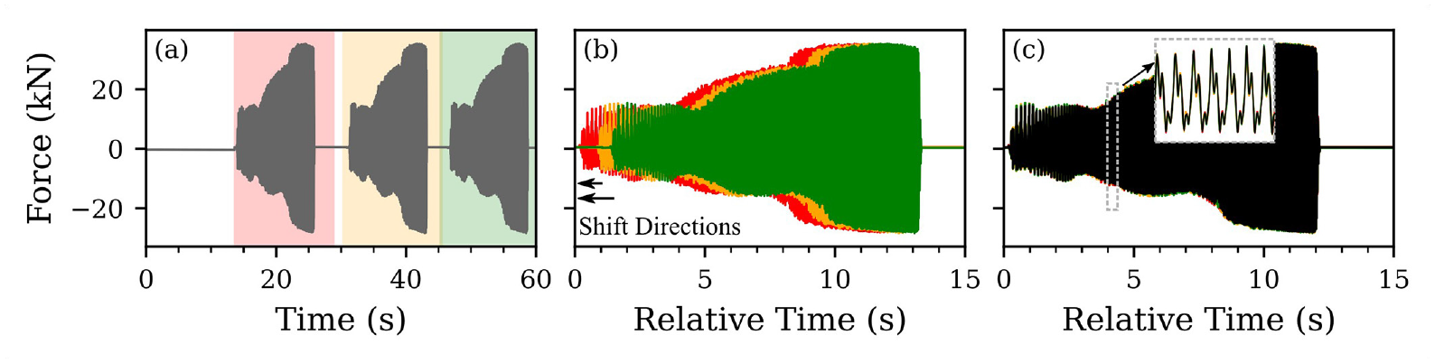
Example of the process used to align individual vibroseis shots prior to stacking. Panel (a) shows the signal recorded from the vibroseis for 60 s following the start time noted in the field at vibroseis source location 57. The three shaded areas denote the manually selected, 15-s windows that contain the three vibroseis sweeps performed at this location. Panel (b) shows the three, 15-s windows plotted relative to their selected start time from panel (a). The direction of the cross-correlation time shifts relative to the first recorded shot is indicated with black horizontal arrows. Panel (c) shows the three source signals aligned using the time shifts determined from cross-correlation. The solid black line indicates the average or “stack” of the three source signatures.

Figure 7.

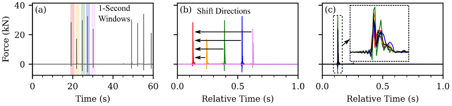
Example of the process used to align individual sledgehammer shots prior to stacking. Panel (a) shows the signal recorded from the instrumented sledgehammer for 60 s following the start time noted in the field at hammer source location 168. The five shaded areas denote the manually selected, 1-s windows that contain the five source impacts performed at the source location. Panel (b) shows the five, 1-s windows plotted relative to their selected start time from panel (a). The direction of the cross-correlation time shifts relative to the first recorded shot is indicated with black horizontal arrows. Panel (c) shows the five source signals aligned using the time shifts determined from cross-correlation. The solid black line indicates the average or “stack” of the five source signatures.

The individual times of each source impact per source location needed to be identified. To do this, we manually selected the approximate start time of each source impact, shown as the left-hand border of the 15- and 1-s shaded windows in Figures 6a and 7a, respectively. Note that while this process could likely have been fully automated, the choice of doing it manually was made for two main reasons. The first was that several of the source locations, especially the hammer source locations, included extra shots (i.e. more than five) that were not listed on the datasheet (a consequence of miscounting in the field), and as such required human-level interpretation to separate the shots. The second was to ensure each source signature was visually reviewed for quality. The process to approximately select the beginning time for all 1300 source signatures took roughly 6 h. These approximate, manually selected beginning times for each shot became the new zero times for each shot on a relative time scale (refer to Figures 6b and 7b). Then, they were cross-correlated to identify the number of time shifts required to align them for subsequent stacking. This process is shown in Figures 6b and 7b, where all source signatures are plotted relative to their picked times from Figures 6a and 7a, respectively, and arrows denote the direction and magnitude of their shifts calculated using cross-correlation relative to the first source signature. These shifts were then applied to align the source signatures prior to stacking. The aligned source signatures and the stacked source signature are shown in Figures 6c and 7c. Note that the black line indicates the average or “stacked” source signature and it overlaps so well with the individual aligned shots that it is difficult to view them all. With the source signatures shifted in preparation for stacking, it was now possible to determine the absolute start time for each source impact by taking the nearest minute written in the field, adding to it the manually picked time relative to that minute, and finally adding the cross-correlation time shifts. The aforementioned process provided the absolute time that denoted the start of each source impact required for relating the source and receiver station data.

While the absolute times derived above could have been used to extract each source record directly from the IRIS DMC, an alternate but equivalent approach was used. This alternate approach involved downloading short blocks of time before and after each source start time noted in the field (one for each station for each source position). Having the raw data stored locally allowed revisions to the post-acquisition processing workflow without requiring the data to be downloaded again from the IRIS DMC (a time-consuming process). To provide data for the most likely processing scenarios, it was decided to include the waveform recordings from all stations for all interior shots (e.g. for FWI) and to provide waveform recordings associated with its corresponding line (see Figure 2a) for all exterior shots (e.g. for MASW). Note that while exterior shots can be used for FWI (e.g. to provide longer ray paths) and the interior shots for MASW (e.g. to provide better spatial sampling), the authors decided the selected approach represents a reasonable simplification that is consistent with most studies. To reduce the size of the active-source data, it was downsampled from 2000 Hz (0.5 ms) to 400 Hz (2.5 ms) during its download from the IRIS DMC. With the data downloaded, the waveforms recorded by each receiver for each source impact were extracted using the cross-correlated source time shifts described above and reviewed. The review process included two data-quality checks. The first was a check on the stacking procedure itself that involved stacking the signals using the closest receiver rather than the source signature. The results from this check were time-domain stacks of the receiver signals that were found to be identical to those obtained using the source signature approach. The second was a check on the quality of the source and receiver signals, which involved viewing the resulting source signature and sampling of receiver waveforms from all 275 source locations and manually removing source impacts that were of very poor quality. Source records were removed if they were contaminated with significant high-amplitude noise, such as from trucks driving down the nearby highway or anthropogenic activity in the storage yard to the south of the array. While quite tedious and time-consuming, this process of removing noisy source impacts was determined to be worthwhile because it resulted in substantially cleaner waveforms. As a result, while three vibroseis and five sledgehammer shots were performed at most source locations, only those deemed of good quality were included in the stacking process. Example waveforms will be presented in the next section of the article on potential use cases of the data set.

The last step of the receiver data post-acquisition processing was to convert the data to engineering units and provide the results in an easy-to-reuse data format. The process of converting data measured with geophones to engineering units is not as straightforward as those described above for the vibroseis and sledgehammer sources, as the geophone’s amplitude and phase response are frequency-dependent. To correct for the instrument’s response, its frequency-dependent amplitude and phase responses must be removed from the recorded waveforms. This is especially important for frequencies near and below the sensor’s resonant frequency, which for the sensors used in this study is 5 Hz. To remove this frequency-dependent effect, IRIS PASSCAL provides the frequency response of each sensor from the manufacturer. Under ideal circumstances, the measured frequency response of each component of each sensor would be used rather than the standard manufacturer-provided response. However, this was not possible for this study, and so we rely on the manufacturer-provided response. The response of each component of these nodal stations can be described with a sensitivity of 4.12E + 09 m/s per count, gain of 0.9998, poles at (−21.99 + 22.43j, −21.99 − 22.43j), and zeros at (0 + 0j, 0 − 0j), where j is the imaginary number. Note the instrument response information has also been included with the published data set in both StationXML and RESP formats. The conversion to physical units was performed using the simulate_seismometer function from the obspy Python package (The ObsPy Development Team, 2022). In addition to the information listed previously, a cosine taper over 5% of the sensor signal (2.5% off either end) and a high-pass filter at 3 Hz with a cosine taper to zero at 2 Hz was applied to mitigate frequency-domain artifacts during the correction process. The results of this process are signals that as closely as possible measure the ground’s true particle velocity in engineering units of m/s. Note that due to the somewhat subjective nature of this process, including the size of the cosine taper and the use of a high-pass filter and its corresponding frequencies, we have provided both the raw data in units of counts (i.e. without any instrument correction performed) and the data in units of m/s (i.e. after the instrument correction as described above has been performed). By providing the data in both formats, we enable users who agree with the choices made above to easily reuse the data, but also accommodate those who wish to use a different instrument correction procedure. The uncorrected and corrected data have been saved in CSV format. The choice to use the CSV format rather than a binary-based format, such as was used for the passive data, was due to the plethora of potential formats for active-source data used in geophysics (e.g. SEG-Y rev1, SEG-Y rev2, SEG-2, SU, etc.) and the fact that there is no clear industry standard for active-source data. For those looking for a versatile binary format, the authors recommend using obspy (The ObsPy Development Team, 2022) to write the data to the Seismic Unix (SU) format. As a result, for each source impact, there are four associated CSV files (one for the source signature and three for the stations (one per component)). In all files, the first column provides a time vector followed by one column for each associated receiver waveform. The header of each column specifies the type of data recorded and in parentheses the units of that data. The entire active-source data set, despite being stored in a text-based format and including the data in both counts and engineering units, is only 25GB and includes approximately 9000 files. The next and final section of this article details the potential use cases of the passive-wavefield and active-source data.

Potential data set use cases

Three-dimensional subsurface imaging via FWI and ambient noise tomography

To illustrate the use of the presented data set for active-source 3D imaging experiments, such as FWI, Figure 8a shows a plan view of a single hammer source location (i.e. 78; refer to Figure 5) relative to a selection of six stations (i.e. 61, 16, 157, 14, 151, and 53; refer to Figure 3). Figures 8b to g show the stacked vertical components of the six selected stations in engineering units, respectively. The recordings show that a sledgehammer source was able to produce clear waveforms across the spatial extents of the array. To illustrate the value of the passive-wavefield measurements for 3D imaging experiments, such as ambient noise tomography (ANT), Figure 9 presents the cross-correlation waveforms for 4 h of ambient noise between all stations and Station 1. More specifically, 4 h of ambient noise (UTC: 2019_10_09T10 to 2019_10_09T13) recorded by each station was filtered between 2 and 15 Hz, divided into 3600, 1-s-long time windows, and each window cross-correlated with the corresponding window recorded on Station 1. The resulting 3600 sets of cross-correlation time series for each station were averaged together to produce the average cross-correlation lags presented in Figure 9a by station number and Figure 9b by distance from Station 1. As expected, the coherent surface wave energy is observed to be much stronger at negative time lags, indicating wave energy primarily arriving from the northeast (i.e. in the direction of the nearby highway).

Figure 8.

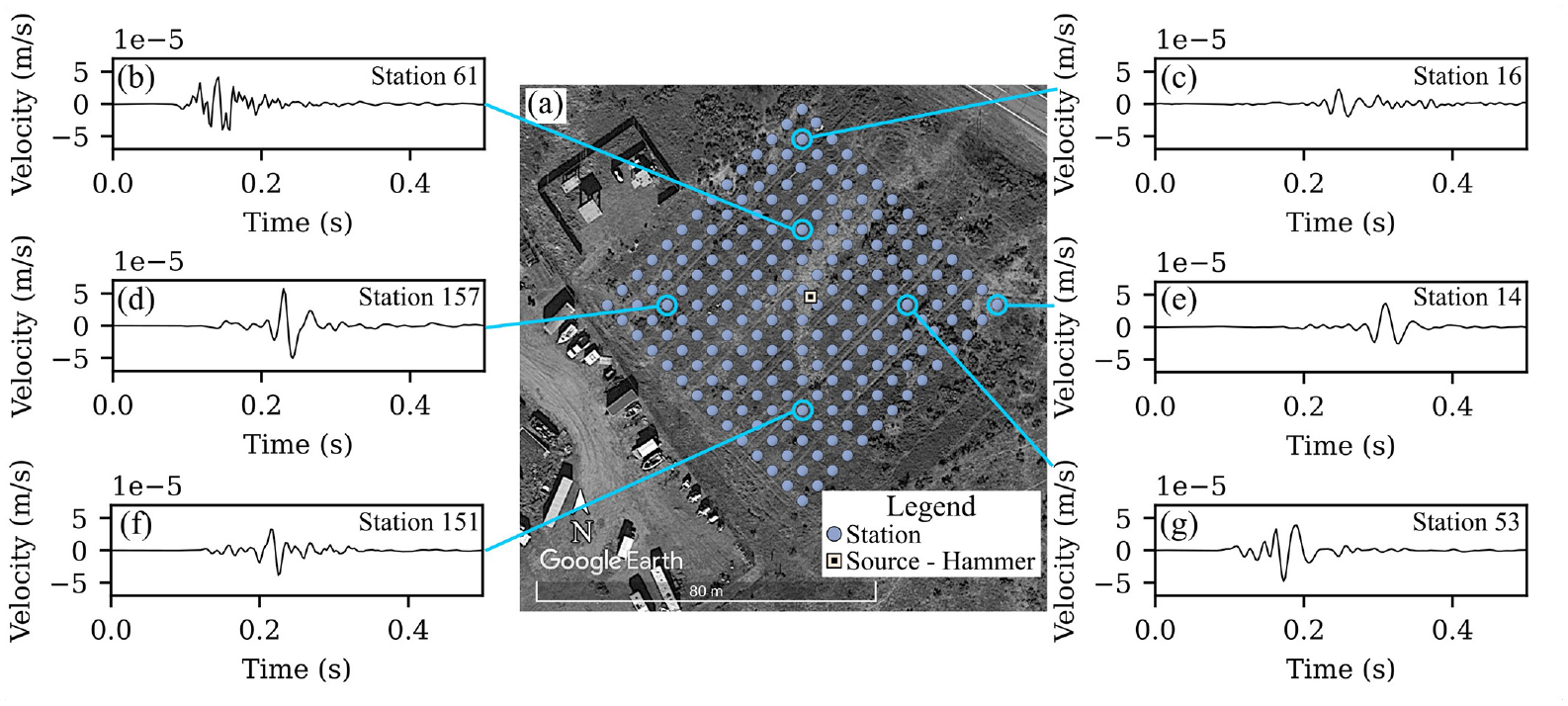
Examples of vertical component waveforms recorded from a single, active-source hammer impact at location 78. Panel (a) shows the location of the example hammer source relative to six example recording locations. Panels (b) to (g) present the stacked vertical component in engineering units from the six stations (i.e. 61, 16, 157, 14, 151, and 53, respectively).

Figure 9.

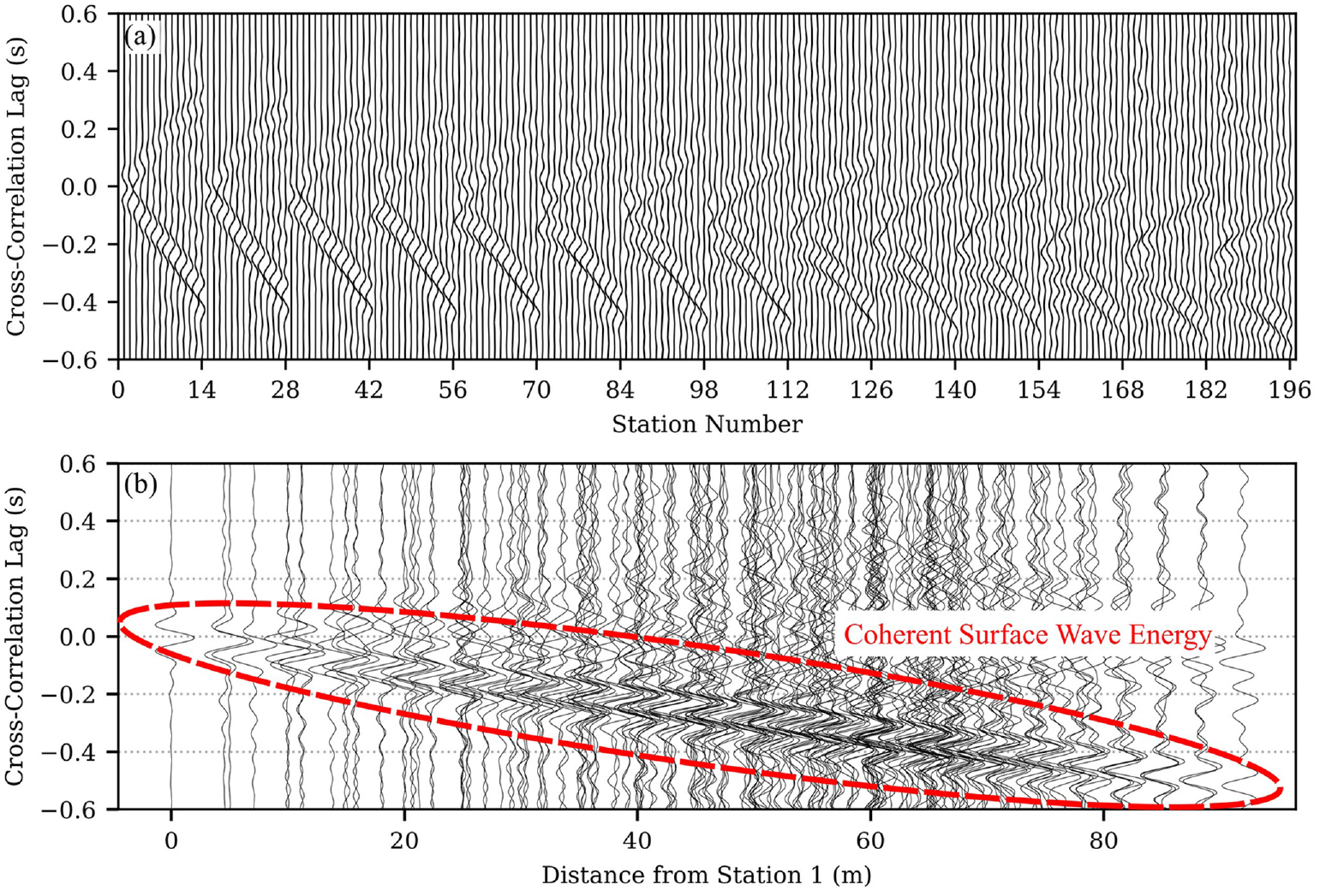
Average cross-correlation between the vertical components of all 196 stations and Station 1 produced from 4 h of ambient noise using a 1-s-long time window. Results are presented by station number in panel (a) and by distance from the Station 1 (i.e. the reference station) in panel (b).

Horizontal-to-Vertical Spectral Ratio

The passive-wavefield data set can also be used to calculate horizontal-to-vertical spectral ratios (HVSRs). To illustrate, Figure 10b shows the 196 stations color-mapped in terms of their fundamental natural frequency from the HVSR median curve (f_0,mc) using HVSR computed from 1 h (UTC: 2019_10_09T10) of ambient noise. The calculation was performed using the open-source Python package hvsrpy (Vantassel, 2021a) and involved dividing the 1-h-long recording into 120-s-long time windows, combining the horizontal components using the geometric mean, as recommended by Cox et al. (2020), smoothing with the filter proposed by Konno and Ohmachi (1998) with b = 40, and calculating the lognormal median (LM) and ± one lognormal standard deviation (STD) curves. The peak of the lognormal median curve (f_0,mc) was used for simplicity instead of the more rigorous calculation of fundamental frequency from the peaks of individual time windows. From Figure 10b, we observe some variability in f_{0, mc} across the site, with values ranging from 1.83 to 1.95 Hz. Figure 10a and c show the calculated HVSR in greater detail for Stations 1 and 169, respectively. In both examples, we observe two peaks in the HVSR; one at approximately 2 Hz and one at approximately 3 Hz. The authors note that these closely spaced peaks may be indicative of the two impedance contrasts between the AL/DG and the DG/GR that are known to exist at the GVDA site. However, we have also observed azimuthal variability in these peaks and they may correspond to valley longitudinal versus valley perpendicular directions. Thus, further investigations are required to more clearly understand the meanings of the HVSR curves.

Figure 10.

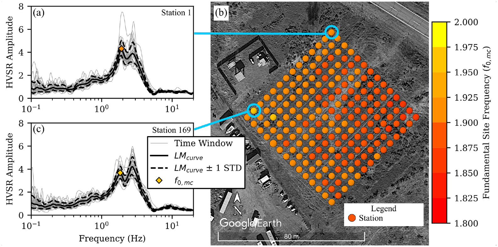
Example HVSR data calculated using 1 h of ambient noise. Panels (a) and (c) show detailed plots of HVSR curves computed at Stations 1 and 169, respectively, including the individual HVSR curves from each 120-s time window, the lognormal median curve ( $L{M}_{\mathrm{curve}}$ ) ± 1 lognormal standard deviation (STD), and the fundamental site frequency from the median curve ( $f_{0,\mathrm{mc}}$ ). Panel (b) shows the spatial distribution of $f_{0,\mathrm{mc}}$ across all stations.

MASW

The hammer and vibroseis source locations positioned outside of the array (i.e. the exterior shots) can be used for MASW as a means to invert for shallow 1D shear wave velocity structure beneath each linear array of receivers. Figure 11a and b show time-domain stacked waveforms from two of the eight hammer source locations associated with lines EW07 and NS07, respectively. The location of each array line is illustrated in Figure 11c. Note the waveforms in Figure 11a and b are from source locations 134 and 160 (refer to Figure 5), located 7.5 m away from the first geophone to the array’s southeast and southwest, respectively. The surface wave dispersion images resulting from transforming the waveforms from Figure 11a and b are shown in Figure 11d and e. The wavefield transformation used is the frequency-domain beamformer (FDBF) with cylindrical-wave steering vector and square-root-distance weighting, as developed by Zywicki and Rix (2005) and implemented in the open-source Python package swprocess (Vantassel, 2021b). The MASW data along both lines are broadband with clear, apparently fundamental-mode Rayleigh (R0) dispersion data between 5 and 60 Hz. Due to the relatively large receiver spacing of 5 m, some spatial aliasing is observed at high frequencies (> 50 Hz). The authors note that an apparently first higher-mode Rayleigh (R1) dispersion trend is also visible, although faint, in both dispersion images and has been denoted as (R1?) in the figures.

Figure 11.

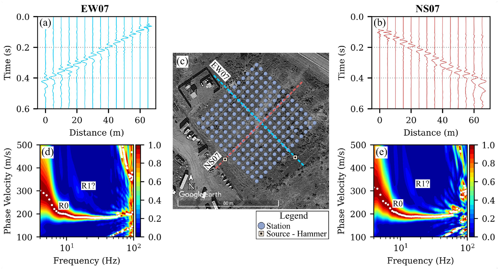
Example MASW data using two exterior hammer source locations. Panels (a) and (b) show the stacked vertical component waterfall plots associated with lines EW07 and NS07 for hammer source locations 134 and 160, respectively. Panel (c) shows a plan view of the GVDA site with the aforementioned linear arrays and shot locations indicated. Panels (d) and (e) show the dispersion images obtained from the waveforms in (a) and (b), respectively, after being transformed to the frequency-phase velocity domain using the FDBF with cylindrical-wave steering vector and square-root-distance weighting. The fundamental Rayleigh mode (R0) and potentially the first-higher Rayleigh mode (R1?) are labeled accordingly.

MAM

The passive-wavefield recordings can also be used for MAM as a means to invert for deep 1D Vs structure beneath the entire array. While all 196 stations and all 28 h of ambient noise data can be processed simultaneously, the computational demands in terms of memory and runtime exceed those pertinent for this preliminary demonstration of the data. Instead, a sampling of the stations and 1 h (UTC: 2019_10_09T10) of ambient noise data will be used. To examine lower frequency dispersion data than from the MASW shown previously, a 60-m diameter circular array (C60) was constructed from 36 of the 196 stations. Stations for the C60 array were selected by finding all stations inside of two bounding circles of diameter 54 and 64 m. The bounding circles and the 36 selected stations are shown in Figure 12a. The ambient noise data were processed using the Rayleigh three-component beamformer (RTBF) method developed by Wathelet et al. (2018) and implemented in the open-source software geopsy (Wathelet et al., 2020). The RTBF processing used fixed-length, 30-s blocks combined into block sets of size 30. To accommodate the limited data used for this example (i.e. only 1 of 28 possible hours of noise), block sets were allowed to overlap up to 29 blocks. Up to five peaks were stored at each processing frequency. The results of the RTBF processing were post-processed using the open-source Python package swprocess (Vantassel, 2021b). The fundamental-model Rayleigh and Love-wave dispersion data (i.e. R0 and L0) after interactive trimming to remove outliers and calculate statistics (Vantassel and Cox, 2022) are presented in Figure 12b and c, respectively. The R0 data are observed to be consistent with the MASW results for common frequencies (refer to Figure 11d and e). Furthermore, as expected from surface wave theory, the Rayleigh wave phase velocity data start to cross below the Love wave data at high frequencies (approximately 13 Hz). The authors note that the Love wave data’s extension to frequencies below that of the Rayleigh wave data (i.e. to longer wavelengths) indicates that Love wave data may help better constrain deeper Vs profiles developed at GVDA in the future.

Figure 12.

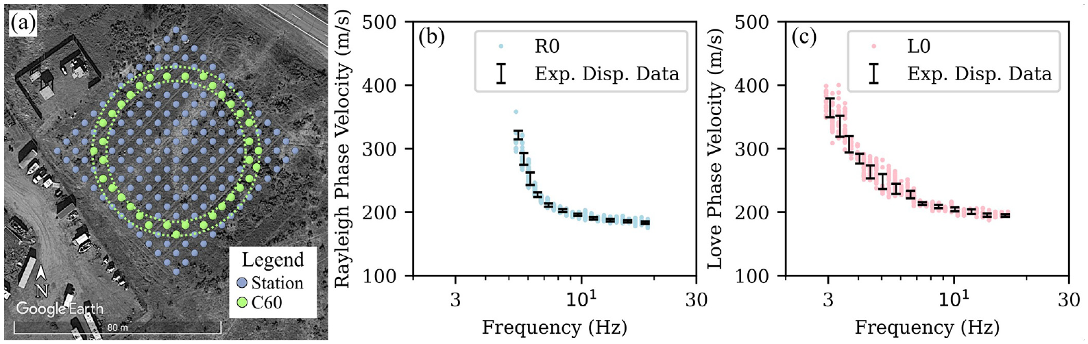
Example MAM made using 1 h of passive-wavefield data from 36 of the 196 stations. The stations, which were selected to roughly correspond to a circular array with a diameter of 60 m (i.e. C60), are shown in panel (a). Panels (b) and (c) show the fundamental Rayleigh (R0) and fundamental Love (L0) wave dispersion data, respectively, extracted from the array noise measurements using the RTBF. Note that the dispersion data are shown after interactive trimming to remove outliers and alongside its associated mean and one standard deviation range.

Conclusion

This article presents a large-scale data set for near-surface imaging acquired at the GVDA site. The data set includes active-source and passive-wavefield recordings made using 196 3C nodal stations positioned on a 14 × 14 grid with a 5 m spacing. All stations were oriented to magnetic north and buried to ensure good coupling. The active-source data include 66 vibroseis and 209 instrumented sledgehammer source locations. All active-source measurements include the recorded source signature and 3C station data in both counts and engineering units (i.e. kN) saved in an easy-to-reuse CSV format. Multiple source impacts were recorded at each source location and prepared for stacking but stored as separate CSV files (i.e. in their unstacked form) to enable future reuse. The passive-wavefield data include 28 h of ambient noise recorded over two nighttime deployments. The passive-wavefield data are saved in 1-h time blocks for each station (all three components saved in a single file) in the easy-to-reuse miniSEED format. The data set is shown to be useful for active-source and passive-wavefield 3D imaging and other subsurface characterization techniques, which include HVSRs, MASW, and MAM. The authors hope that making this unique data set available will help accelerate work in 3D subsurface imaging for near-surface engineering applications.