Sage Journals: Discover world-class research

Abstract

In this study, we derived a regionalized partially nonergodic empirical ground-motion model (GMM) for subduction interface and intraslab earthquakes using an extensive global database compiled as part of the NGA-Subduction project. The model can be used to estimate peak ground acceleration (PGA), peak ground velocity (PGV), and ordinates of 5%-damped pseudo-spectral acceleration (PSA) at periods ranging from 0.01 to 10 s for M ≥ 5.0, M≤ 8.5 for intraslab events, M≤ 9.5 for interface events, Z_TOR≤ 50 km for interface events, Z_TOR≤ 200 km for intraslab events, 10 ≤R_RUP≤ 800 km, and 100 ≤V_S₃₀≤ 1000 m/s. Besides a global version of the model, the GMM accounts for regional differences in the overall amplitude (constant), anelastic attenuation, linear site response, and basin response for seven subduction-zone regions: Alaska (AK), Central America and Mexico (CAM), Cascadia (CASC), Japan (JP), New Zealand (NZ), South America (SA), and Taiwan (TW). The functional form of the model is structured such that the breakpoint magnitude, the magnitude at which the magnitude-scaling rate (MSR) transitions from a steeper to a shallower slope, is an adjustable parameter in the model. This makes it possible to take epistemic uncertainty in this parameter into account or adjust it based on other empirical or physical information, such as when the model is applied to a subduction zone not considered in the GMM. Besides the traditional mixed-effects aleatory between-event standard deviations and within-event standard deviations, within-model epistemic standard deviations in the median prediction for each region is quantified from a posterior distribution of model coefficients, standard deviations, and coefficient correlations using a Bayesian regression approach. Our full 800-sample posterior distribution can be used to account for epistemic uncertainty in the model coefficients, standard deviations, and predicted values. We also provide a simplified epistemic model using magnitude- and distance-dependent within-model standard deviations that can be used to facilitate the inclusion of within-model epistemic uncertainty directly in a probabilistic seismic hazard analysis. The within-model standard deviations can also be used to scale the GMM using a backbone modeling approach.

Keywords

Bayesian model ground-motion model nonergodic GMM seismic hazard subduction

Introduction

Subduction zones can produce very large megathrust earthquakes and, thus, pose a significant seismic risk in many regions of the world. Since ground-motion models (GMMs) are an integral part of probabilistic seismic hazard analysis (PSHA), the development of GMMs for subduction earthquakes is of major importance to accurately quantify the seismic hazard from such events. This has led to the development of several empirical and simulation-based GMMs over the years for both interface and intraslab subduction earthquakes. The models based on stochastic or physics-based ground-motion simulations are typically developed for a specific application to a localized region, such as the CASC in the Pacific Northwest of the United States (Atkinson and Macias, 2009; Gregor et al., 2002), whereas many empirical models are developed for more global applications (Abrahamson et al., 2016; Abrahamson and Gulerce, 2022; Atkinson and Boore, 2003, 2008; Parker et al., 2022) or for regions where there are an abundance of recordings, such as Chile (Fayaz et al., 2023; Idini et al., 2017; Macedo and Liu, 2022; Montalva et al., 2017, 2022), Ecuador (Arteta et al., 2021), Greece (Kkallas et al., 2018), JP (Campbell et al., 2022; Ghofrani and Atkinson, 2014; Hassani and Atkinson, 2021; Morikawa and Fujiwara, 2013; Si et al., 2022; Zhao et al., 2006, 2016a, 2016b), and TW (Chao et al., 2020; Phung et al., 2020).

In this article, we summarize a regionalized partially nonergodic empirical GMM that was developed by Kuehn et al. (2020a) as part of the Next Generation Attenuation (NGA) research project on subduction earthquakes (Bozorgnia et al., 2022), hereafter referred to as NGA-Sub. We refer to this model as KBCG20 throughout the article. KBCG20 can be used to predict the RotD50 horizontal component (Boore, 2010) of peak ground acceleration (PGA), peak ground velocity (PGV), and ordinates of 5%-damped pseudo-spectral acceleration (PSA) at 21 periods ranging from 0.01 to 10 s. Details about the model and modeling approach is available in the study by Kuehn et al. (2020a), although we note that some of the coefficients from that study have since been modified. We regionalized the GMM for seven subduction-zone regions with special attention to CASC, because of the limited number of earthquakes from this latter region and its importance to seismic hazards in the Pacific Northwest of the United States (Petersen et al., 2020). In particular, KBCG20 was developed as a partially nonergodic model similar to the approach described in Stafford (2014), which means that some terms in the model vary by region while other terms are shared among the regions. The model parameters are estimated using Bayesian inference (Gelman et al., 2013; Spiegelhalter and Rice, 2009), which allows the inclusion of prior information in a probabilistic way. We also place strong emphasis on the estimation of within-model epistemic uncertainty, which is estimated from a posterior distribution of model parameters derived from the Bayesian regression.

Database

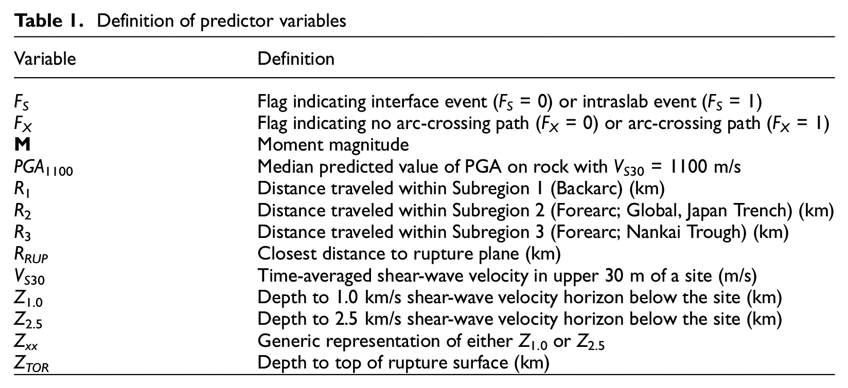
We used a subset of the NGA-Sub database based on a set of selection criteria designed to include only those data that are deemed to be accurate, reliable, and usable for GMM development (Kuehn et al., 2020a). The predictor variables included in KBCG20 are summarized in Table 1. Our data selection and exclusion criteria are listed below.

Table 1.

Definition of predictor variables

Variable	Definition
F_S	Flag indicating interface event (F_S = 0) or intraslab event (F_S = 1)
F_X	Flag indicating no arc-crossing path (F_X = 0) or arc-crossing path (F_X = 1)
M	Moment magnitude
PGA ₁₁₀₀	Median predicted value of PGA on rock with V_S₃₀ = 1100 m/s
R ₁	Distance traveled within Subregion 1 (Backarc) (km)
R ₂	Distance traveled within Subregion 2 (Forearc; Global, Japan Trench) (km)
R ₃	Distance traveled within Subregion 3 (Forearc; Nankai Trough) (km)
R_RUP	Closest distance to rupture plane (km)
V_S ₃₀	Time-averaged shear-wave velocity in upper 30 m of a site (m/s)
Z _1.0	Depth to 1.0 km/s shear-wave velocity horizon below the site (km)
Z _2.5	Depth to 2.5 km/s shear-wave velocity horizon below the site (km)
Z_xx	Generic representation of either Z_1.0 or Z_2.5
Z_TOR	Depth to top of rupture surface (km)

Inclusion criteria:

Interface (F_S = 0); intraslab (F_S = 1), or the lower part of a double seismicity intraslab zone (F_S = 5). The latter two are combined and referred to simply as intraslab or slab events (F_S = 1). Contreras et al. (2022) provides details on event classification in the NGA-Sub database.

Magnitudes of M > 4.0 which, although may not be of engineering interest, includes smaller magnitudes and an increased number of recordings that helps to constrain many of the model parameters in the regression analyses.

Ratios of the largest to smallest rupture distance larger than 2, which ensures that each event has a reasonable distance range that allows a reliable estimate of event terms and attenuation parameters.

Recordings with non-missing values of moment magnitude (M), rupture distance (R_RUP), time-averaged shear-wave velocity in the upper 30 m of the site (V_S₃₀), and depth to the top of the rupture surface (Z_TOR).

Recordings with a minimum rupture distance of R_RUP < 800 km or R_RUP < R_MAX if smaller, where R_MAX is the minimum distance to non-triggered recordings for each event, which arises when an instrument triggers only above a certain amplitude threshold (see Contreras et al., 2022).

Exclusion criteria:

6. Predictor variables other than basin depths with missing values.

7. Stations with an instrument depth > 2 m to avoid depletion of high-frequencies due to embedment effects.

8. Recordings with PGA > 10 g, which likely represent incorrect instrument gains or other errors.

9. Recordings with a multiple event flag equal to 1 representing recordings with more than one recorded earthquake.

10. Recordings with a visual quality flag equal to 2 representing a late S-trigger or 9 representing non-useable data.

11. Recordings with a GMX site classification first letter code of N, Z, or F representing non-free-field stations.

We do not discard recordings from stations with no estimate of Z_1.0 or Z_2.5. These so-called basin or sediment depths are only available for a limited number of stations and regions. Discarding these stations would severely reduce the number of usable data. Furthermore, where they are available, including them in the regression was found to significantly reduce the within-event aleatory variability at long periods.

For CASC, two events were classified as interface earthquakes in the database. Located off the central Oregon coast, they have magnitudes of M = 4.7 and M = 4.9. After discussions with the NGA-Sub project researchers and the USGS National Seismic Hazard Model Program, and considering the questionable classification of these events as interface events, these earthquakes were excluded from our database.

We also excluded the 4 October 1994 M 8.28 Kuril event because of its location on the outer rise of the Kurile Subduction Zone and its thrust-oblique focal mechanism (Tanioka et al., 1995), which is inconsistent with other Benioff-zone normal-faulting intraslab events included in the database. Based on an initial regression, we also removed all recordings with absolute residuals that deviated more than four times the within-event standard deviation from the median prediction at eight selected periods of engineering interest. This latter criterion was a NGA-Sub project team decision to remove those events and recordings with potential errors in instrument properties or other metadata. After all of the aforementioned criteria were applied, we selected those events that had at least five recordings to allow the calculation of reliable event terms. No such criterion was applied to the number of recordings per station.

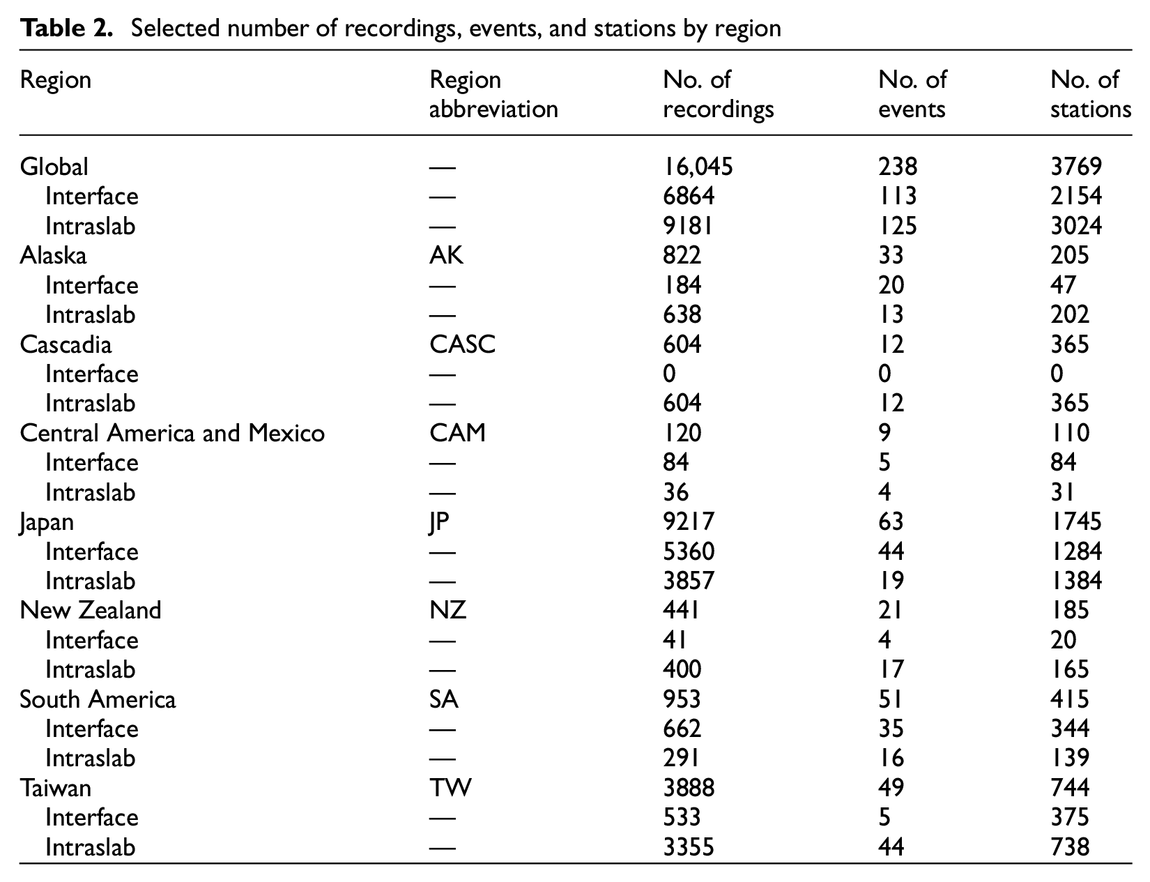
The selected database has a maximum of 16,045 three-component recordings from 238 events and 3769 recording stations. There are 6864 recordings from 113 interface events and 9181 recordings from 125 intraslab events. At long periods, the number of recordings is reduced due to a smaller useable bandwidth. Table 2 lists the number of recordings, number of events, number of stations, and region abbreviation for each of the subduction regions for the subset of NGA-Sub data selected for analysis. JP dominates the data set with over 50% of the recordings. TW and SA also have a significant number of events but fewer recordings per event than JP. The number of available recordings for CASC, CAM, and NZ is relatively sparse. The magnitude–distance distribution of the data is shown in Figure 1.

Table 2.

Selected number of recordings, events, and stations by region

Region	Region abbreviation	No. of recordings	No. of events	No. of stations
Global	—	16,045	238	3769
Interface	—	6864	113	2154
Intraslab	—	9181	125	3024
Alaska	AK	822	33	205
Interface	—	184	20	47
Intraslab	—	638	13	202
Cascadia	CASC	604	12	365
Interface	—	0	0	0
Intraslab	—	604	12	365
Central America and Mexico	CAM	120	9	110
Interface	—	84	5	84
Intraslab	—	36	4	31
Japan	JP	9217	63	1745
Interface	—	5360	44	1284
Intraslab	—	3857	19	1384
New Zealand	NZ	441	21	185
Interface	—	41	4	20
Intraslab	—	400	17	165
South America	SA	953	51	415
Interface	—	662	35	344
Intraslab	—	291	16	139
Taiwan	TW	3888	49	744
Interface	—	533	5	375
Intraslab	—	3355	44	738

Figure 1.

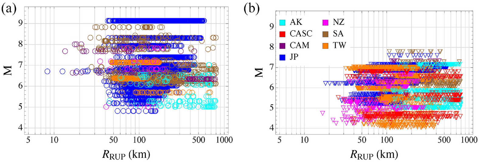
Magnitude and distance distribution of data from (a) interface and (b) intraslab events with separate colors for the seven modeled subduction regions.

Ground-motion model

The GMM is developed as a Bayesian multi-level/hierarchical model (Gelman and Hill, 2006). This means that we recognize that there are different levels in the data that can be exploited during the model-building process. Each level consists of data that can be grouped according to some criterion, such as by event or geographic region. The levels form the following hierarchy from broadest to narrowest: global → regional → event → recording. Within each level, some parameters are shared within groups, such as the event term for all recordings from the same event, while others are taken from higher levels. The inclusion of the regional, event, and recording levels allows us to relax the ergodic assumption that all recordings come from the same population by associating them with groups or hierarchical levels (Anderson and Brune, 1999), leading to what is referred to as a partially nonergodic model (Stafford, 2014).

The coefficients that are regionalized in KBCG20 are those related to the overall amplitude (constant), anelastic attenuation, linear site response, and basin response. The constant, linear site response, and anelastic attenuation are modeled as regional random effects (Stafford, 2014). The basin response is modeled as an adjustment to the final regional GMM. Because basin depths are not available for all regions and for all sites within a region, they were estimated from the regional within-event residuals of the model. We describe the regionalization of the model in more detail in the “Geographic regionalization” section of the article.

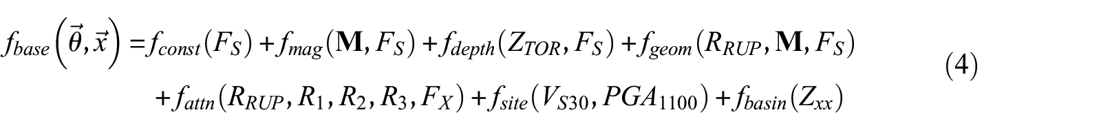
Base model

At the recording level, the model assumes that the target ground-motion variable $\ln Y$ is distributed according to a normal or Gaussian distribution given by its mean µ and standard deviation ϕ:

\ln Y ~ N (μ, ϕ)

(1)

μ = f_{base} (\vec{θ}, \vec{x}) + δ B

(2)

where µ is the sum of the natural logarithmic median base function $f_{base} (\vec{θ}, \vec{x})$ and an event term δB. The event terms have the following normal distribution with mean zero and standard deviation τ:

δ B ~ N (0, τ)

(3)

The mean prediction $f_{base} (\vec{θ}, \vec{x})$ depends on the model coefficients $\vec{θ}$ (see Table 3) and the predictor variables $\vec{x}$ (see Table 1) defined by the relationship:

\begin{matrix} f_{base} (\vec{θ}, \vec{x}) = & f_{const} (F_{S}) + f_{mag} (M, F_{S}) + f_{depth} (Z_{TOR}, F_{S}) + f_{geom} (R_{RUP}, M, F_{S}) \\ + f_{attn} (R_{RUP}, R_{1}, R_{2}, R_{3}, F_{X}) + f_{site} (V_{S 30}, PG A_{1100}) + f_{basin} (Z_{xx}) \end{matrix}

(4)

Table 3.

Description of model coefficients

Coefficient	Description	Regionalized
θ _1,if	Interface constant	Yes
θ _1,slab	Intraslab constant	Yes
θ _2,if	Interface geometrical attenuation	No
θ _2,slab	Intraslab geometrical attenuation	No
θ ₃	Magnitude-dependent interface and intraslab geometrical attenuation	No
θ _4,if	Interface small-event magnitude scaling rate, MSR	No
θ _4,slab	Intraslab small-event MSR	No
θ ₅	Interface and intraslab large-event MSR	No
θ _6,xc	Arc-crossing constant offset	No
θ _6,x1	Anelastic attenuation within backarc region 1 after crossing a volcanic arc	Yes
θ _6,x2	Anelastic attenuation within forearc region 2 after crossing a volcanic arc	Yes
θ _6,x3	Anelastic attenuation within forearc region 3 after crossing a volcanic arc	Yes
θ _6,1	Anelastic attenuation within backarc region 1 without crossing a volcanic arc	Yes
θ _6,2	Anelastic attenuation within forearc region 2 without crossing a volcanic arc	Yes
θ _6,3	Anelastic attenuation within forearc region 3 without crossing a volcanic arc	Yes
θ ₇	Linear site amplification (V_S₃₀ scaling)	Yes
θ _9,if	Interface source depth-scaling rate, DSR (Z_TOR scaling)	No
θ _9,slab	Intraslab DSR (Z_TOR scaling)	No
θ ₁₀	Source DSR for deep events (Z_TOR > z_B)	No, fixed at zero
θ _11,SEA	Basin-depth constant for Seattle basin	No
θ ₁₁	Basin depth-scaling constant for basins other than Seattle basin	Yes
θ ₁₂	Basin depth-scaling slope for basins other than Seattle basin	Yes
θ_nft,₁	Near-fault pseudo-depth magnitude-scaling term constant	No
θ_nft,₂	Near-fault pseudo-depth magnitude-scaling term slope	No
Z_B,if	Interface adjustment to depth-scaling slope break point	No
Z_B,slab	Intraslab adjustment to depth-scaling slope break point	No

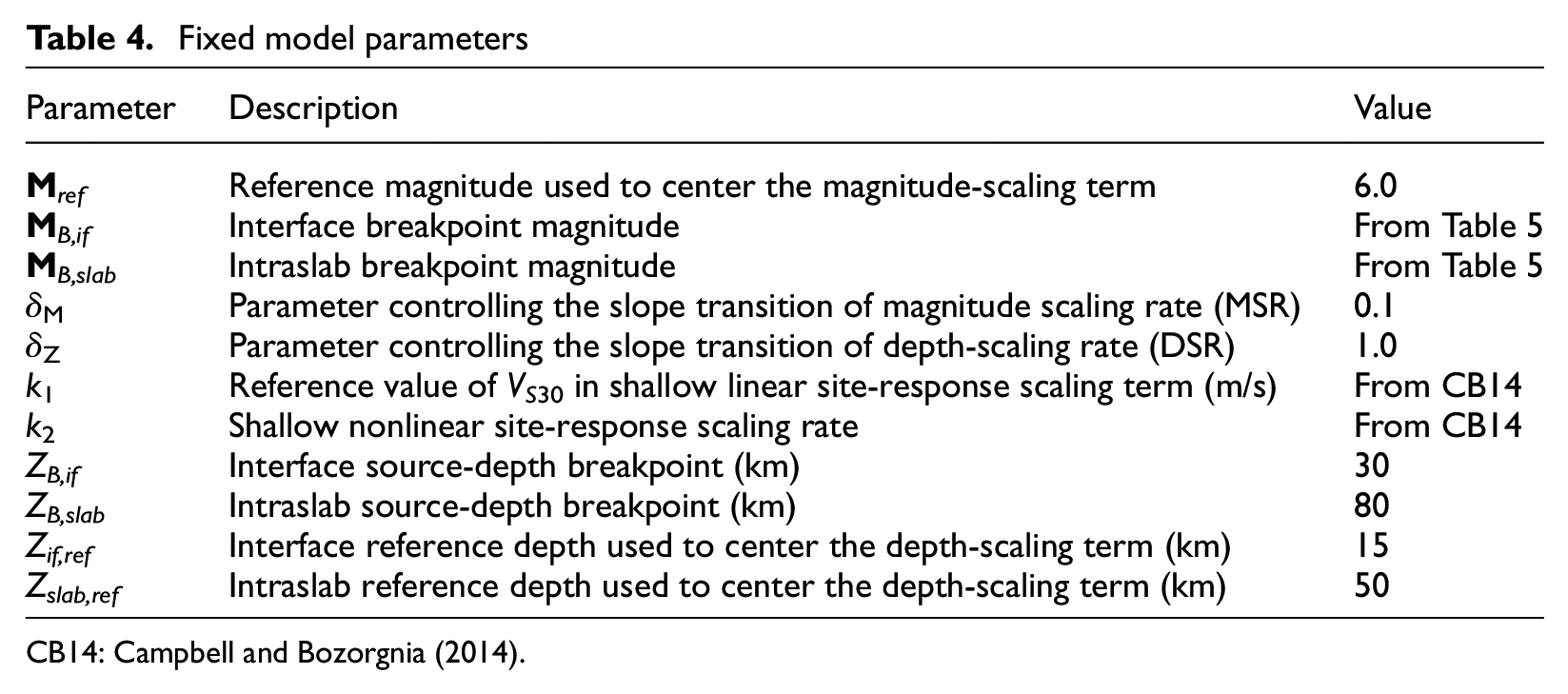
Table 3 also identifies which of the coefficients are regionalized. In addition to the estimated coefficients, there are a few coefficients that are fixed (see Table 4). To ensure a physically meaningful spectrum, the predicted median PSA at short periods is not allowed to be smaller than PGA as given by the equation:

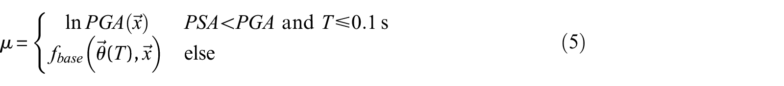
μ = {\begin{matrix} \ln PGA (\vec{x}) & PSA < PGA and T \leq 0.1 s \\ f_{base} (\vec{θ} (T), \vec{x}) & else \end{matrix}

(5)

where $\vec{θ}$ is replaced with $\vec{θ} (T)$ to indicate that the coefficients are a function of period. The parenthetic T is dropped in the remainder of the article for simplicity.

Table 4.

Fixed model parameters

Parameter	Description	Value
M _ref	Reference magnitude used to center the magnitude-scaling term	6.0
M _B,if	Interface breakpoint magnitude	From Table 5
M _B,slab	Intraslab breakpoint magnitude	From Table 5
δ _M	Parameter controlling the slope transition of magnitude scaling rate (MSR)	0.1
δ _Z	Parameter controlling the slope transition of depth-scaling rate (DSR)	1.0
k ₁	Reference value of V_S₃₀ in shallow linear site-response scaling term (m/s)	From CB14
k ₂	Shallow nonlinear site-response scaling rate	From CB14
Z_B,if	Interface source-depth breakpoint (km)	30
Z_B,slab	Intraslab source-depth breakpoint (km)	80
Z_if,ref	Interface reference depth used to center the depth-scaling term (km)	15
Z_slab,ref	Intraslab reference depth used to center the depth-scaling term (km)	50

CB14: Campbell and Bozorgnia (2014).

Logistic hinge function

A bilinear logistic hinge function is used in several of the terms listed in Equation 4. It provides a smooth transition from one slope to another. It is defined by the equation:

lh (x, x_{0}, a, b_{0}, b_{1}, δ) = a + b_{0} (x - x_{0}) + (b_{1} - b_{0}) δ \ln [1 + \exp (\frac{x - x_{0}}{δ})]

(6)

where x₀ is the slope breakpoint, b₀ is the slope for x < x₀, b₁ is the slope for x > x₀, and δ controls the smoothness of the transition between slope b₀ and b₁ with smaller values of δ leading to a sharper transition. The bilinear logistic hinge function is used to model the magnitude-scaling term $f_{mag} (M, F_{S})$ and the depth-scaling term $f_{depth} (Z_{TOR}, F_{S})$ . Compared to a bilinear function that includes a non-continuous logical statement to model different slopes, the logistic hinge function is differentiable everywhere, making it more tractable in a nonlinear regression analysis.

Constant term

The constant term is given by the equation:

f_{const} (F_{S}) = θ_{1, if} (1 - F_{S}) + θ_{1, slab} F_{S}

(7)

which allows a different constant depending on whether the earthquake is an interface or an intraslab event.

Magnitude term

The magnitude-scaling term is modeled by the following bilinear logistic hinge function:

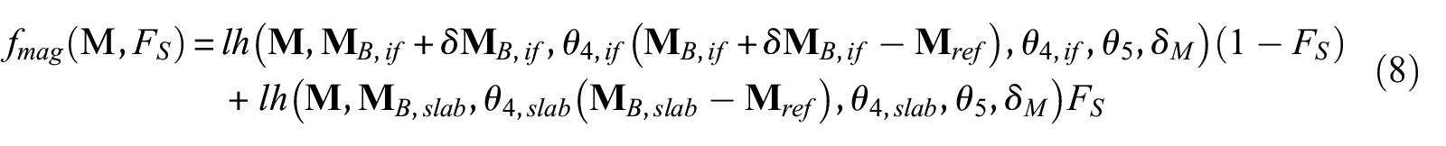
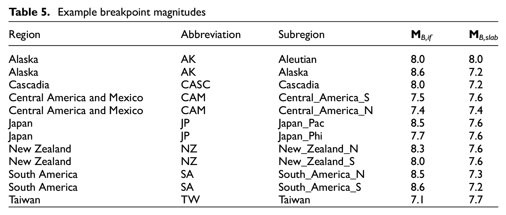
\begin{matrix} f_{mag} (M, F_{S}) = & lh (M, M_{B, if} + δ M_{B, if}, θ_{4, if} (M_{B, if} + δ M_{B, if} - M_{ref}), θ_{4, if}, θ_{5}, δ_{M}) (1 - F_{S}) \\ + lh (M, M_{B, slab}, θ_{4, slab} (M_{B, slab} - M_{ref}), θ_{4, slab}, θ_{5}, δ_{M}) F_{S} \end{matrix}

(8)

The magnitude-scaling functional form is the same for interface and intraslab events, but the model coefficients and fixed parameters are different (see Tables 3 to 5). In particular, the breakpoint magnitude (M_B) and the MSR below the breakpoint magnitude (θ_4,if and θ_4,slab) are different for interface and intraslab events. The MSR above the breakpoint magnitude (θ₅) is assumed to be the same for both interface and intraslab events lacking information to the contrary. The smoothness of the transition between the two linear segments of the scaling relation is fixed at δ_M = 0.1. Preliminary trials to estimate this parameter demonstrated that it was not well constrained and that its posterior distribution was almost unchanged compared to its prior distribution. The selected value leads to a reasonably smooth transition between the two linear segments. The magnitude term has a value of zero at M_ref = 6.0.

Table 5.

Example breakpoint magnitudes

Region	Abbreviation	Subregion	M _B,if	M _B,slab
Alaska	AK	Aleutian	8.0	8.0
Alaska	AK	Alaska	8.6	7.2
Cascadia	CASC	Cascadia	8.0	7.2
Central America and Mexico	CAM	Central_America_S	7.5	7.6
Central America and Mexico	CAM	Central_America_N	7.4	7.4
Japan	JP	Japan_Pac	8.5	7.6
Japan	JP	Japan_Phi	7.7	7.6
New Zealand	NZ	New_Zealand_N	8.3	7.6
New Zealand	NZ	New_Zealand_S	8.0	7.6
South America	SA	South_America_N	8.5	7.3
South America	SA	South_America_S	8.6	7.2
Taiwan	TW	Taiwan	7.1	7.7

During an initial regression, it became apparent that at long periods (T > 1 s), the event terms for interface events at large magnitudes were biased low compared to the observations. As a result, an adjustment to M_B,if for interface events at T > 1 s was modeled similar to that proposed by Abrahamson et al. (2016, 2018). This adjustment is zero at T ≤ 1 s and −0.4 at T ≥ 3 s with a log-linear interpolation in between (i.e. logarithmic in period and linear in the adjustment) as given by the equation:

δ M_{B, if} = {\begin{matrix} 0 & T \leq 1 \\ - 0.4 (T - 1) / 2 & 1 < T < 3 \\ - 0.4 & T \geq 3 \end{matrix}

(9)

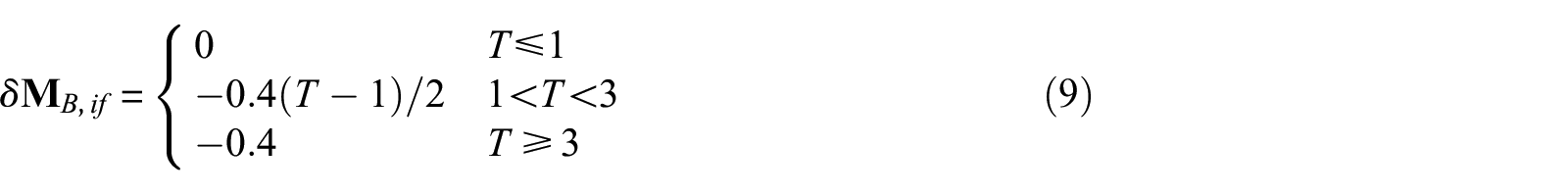
This adjustment is only applied to JP and SA interface events in the regression, since these regions are the only ones with large-enough magnitudes to be effected by this adjustment. However, we believe that there is no reason why it should not be applied to every subduction region in a forward prediction of large-magnitude ground motions.

Geometric attenuation term

The geometric attenuation term (i.e. geometrical spreading) is modeled by the equation:

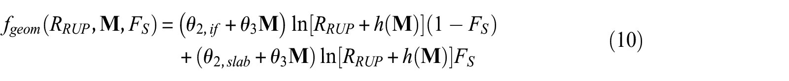
\begin{matrix} f_{geom} (R_{RUP}, M, F_{S}) = & (θ_{2, if} + θ_{3} M) \ln [R_{RUP} + h (M)] (1 - F_{S}) \\ + (θ_{2, slab} + θ_{3} M) \ln [R_{RUP} + h (M)] F_{S} \end{matrix}

(10)

where the finite-fault or “pseudo-depth” term is defined by the equation:

h (M) = 10^{θ_{nft, 1} + θ_{nft, 2} (M - M_{ref})}

(11)

The regression coefficients θ_nft,₁ and θ_nft,₂ are given a relatively strong prior distribution because they are not well-constrained by the data.

Source-depth term

The source-depth term is given by a bilinear logistic hinge function with different slopes and depth breakpoints for interface and intraslab events as follows:

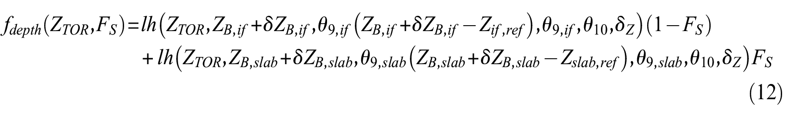
\begin{matrix} f_{depth} (Z_{TOR}, F_{S}) = & lh (Z_{TOR}, Z_{B, if} + δ Z_{B, if}, θ_{9, if} (Z_{B, if} + δ Z_{B, if} - Z_{if, ref}), θ_{9, if}, θ_{10}, δ_{Z}) (1 - F_{S}) \\ + lh (Z_{TOR}, Z_{B, slab} + δ Z_{B, slab}, θ_{9, slab} (Z_{B, slab} + δ Z_{B, slab} - Z_{slab, ref}), θ_{9, slab}, θ_{10}, δ_{Z}) F_{S} \end{matrix}

(12)

where Z_if,ref and Z_slab,ref are reference depths (see Table 4) and δ_Z is the smoothness transition parameter between the two linear slopes. The bilinear DSR has breakpoints at Z_B,if + δZ_B,if and Z_B,slab + δZ_B,slab determined from the regression. The breakpoints were set to Z_B,if = 30 km and Z_B,slab = 80 km based on initial regressions. The period-dependent adjustment coefficients δZ_B,if and δZ_B,slab were determined by regression because the DSR breakpoints have no theoretical basis. The coefficients for the DSR up to the depth breakpoints are θ_9,if and θ_9,slab. Both the coefficients for the DSR above the break points were fixed at θ₁₀ = 0, consistent with the study by Abrahamson et al. (2016, 2018), because there are not many events with depths larger than these breakpoints and those depths that do exist do not show any systematic trend with ground-motion amplitude.

Site-response term

The site-response (site-amplification) term is parameterized as in the study by Campbell and Bozorgnia (2014):

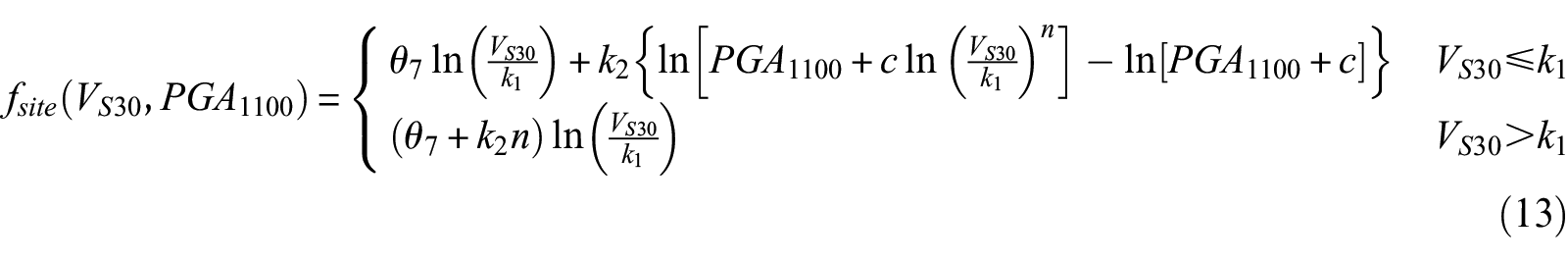
f_{site} (V_{S 30}, PG A_{1100}) = {\begin{matrix} θ_{7} \ln (\frac{V_{S 30}}{k_{1}}) + k_{2} {\ln [PG A_{1100} + c \ln {(\frac{V_{S 30}}{k_{1}})}^{n}] - \ln [PG A_{1100} + c]} & V_{S 30} \leq k_{1} \\ (θ_{7} + k_{2} n) \ln (\frac{V_{S 30}}{k_{1}}) & V_{S 30} > k_{1} \end{matrix}

(13)

The linear site-scaling coefficient θ₇ is a regression coefficient that varies by geographic region. The period-dependent parameters k₁ and k₂, as well as the period-independent constants c and n, are fixed to the values of Campbell and Bozorgnia (2014). Hence, we make the implicit assumption that the nonlinear site amplification for subduction events is similar to that of crustal events, consistent with the assumptions of Abrahamson et al. (2016) and Montalva et al. (2017), although we note that Zhao et al. (2016a, 2016b) Campbell et al. (2022), Parker et al. (2022), and Si et al. (2022) suggest a different site-response term for Japanese recordings.

Anelastic attenuation term

The anelastic attenuation term is defined by the equation:

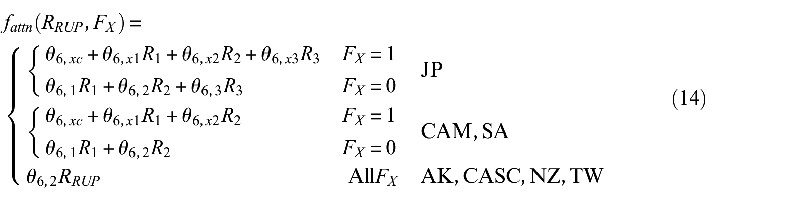
\begin{matrix} f_{attn} (R_{RUP}, F_{X}) = \\ {\begin{matrix} {\begin{matrix} θ_{6, xc} + θ_{6, x 1} R_{1} + θ_{6, x 2} R_{2} + θ_{6, x 3} R_{3} & F_{X} = 1 \\ θ_{6, 1} R_{1} + θ_{6, 2} R_{2} + θ_{6, 3} R_{3} & F_{X} = 0 \end{matrix} & JP \\ {\begin{matrix} θ_{6, xc} + θ_{6, x 1} R_{1} + θ_{6, x 2} R_{2} & F_{X} = 1 \\ θ_{6, 1} R_{1} + θ_{6, 2} R_{2} & F_{X} = 0 \end{matrix} & CAM, SA \\ θ_{6, 2} R_{RUP} & All F_{X} & AK, CASC, NZ, TW \end{matrix} \end{matrix}

(14)

where F_X = 1 when the travel path passes through a volcanic arc (i.e. the transition between the forearc and backarc attenuation subregions) and F_X = 0 otherwise. The regression coefficient θ_6,i represents the anelastic attenuation coefficient for attenuation subregion i before it crosses a volcanic arc. The regression coefficient θ_6,xi represents the anelastic attenuation coefficient for attenuation subregion i after it crosses a volcanic arc. The distance R_i is the distance traveled within each subregion, the sum of which equals R_RUP. The coefficient θ_xc is the offset as the travel path crosses the volcanic arc and θ_6,2 is the attenuation rate for those subduction regions that do not have different attenuation subregions.

The difference in how the subduction regions are modeled is based on inspection of residual plots and ground-motion scaling of trial regressions for each subregion that did not include forearc and backarc attenuation coefficients. Subregion index 1 indicates a travel path within the backarc of JP, CAM, or SA; Subregion 2 indicates a travel path within the forearc of CAM, SA, or northeastern JP; and Subregion 3 indicates a travel path within the forearc of southeastern JP. The northeastern JP forearc sits atop the JP Trench megathrust and the southeastern JP forearc sits atop the Nankai Trough megathrust. Figure 2 shows the attenuation subregions for JP, SA, and CAM.

Figure 2.

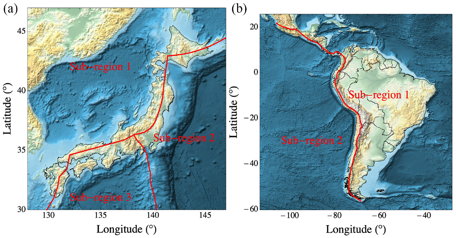
Maps showing anelastic attenuation subregions for (a) Japan and (b) South America and Central America and Mexico.

Basin-response term

The effect of the deep crustal structure beneath the site is modeled with the following basin-response term:

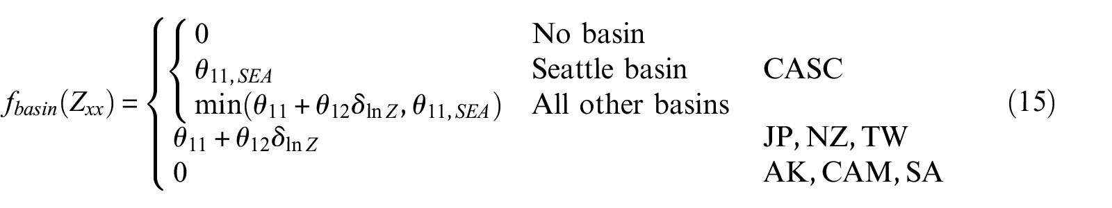
f_{basin} (Z_{xx}) = {\begin{matrix} {\begin{matrix} 0 & No basin \\ θ_{11, SEA} & Seattle basin \\ min (θ_{11} + θ_{12} δ_{\ln Z}, θ_{11, SEA}) & All other basins \end{matrix} & CASC \\ θ_{11} + θ_{12} δ_{\ln Z} & JP, NZ, TW \\ 0 & AK, CAM, SA \end{matrix}

(15)

where Z_xx is either Z_1.0 or Z_2.5 depending on the region, $δ_{\ln Z} = \ln Z_{obs} - \ln Z_{ref} (V_{S 30})$ , Z_obs is the observed value of basin depth, and Z_ref(V_S₃₀) is the reference value of basin depth for a given subduction region and value of V_S₃₀. Z_ref(V_S₃₀) is defined by the equation:

\ln Z_{ref} (V_{S 30}) = θ_{z 1} + (θ_{z 2} - θ_{z 1}) \frac{\exp (\frac{\ln V_{S 30} - θ_{z 3}}{θ_{z 4}})}{1 + \exp (\frac{\ln V_{S 30} - θ_{z 3}}{θ_{z 4}})}

(16)

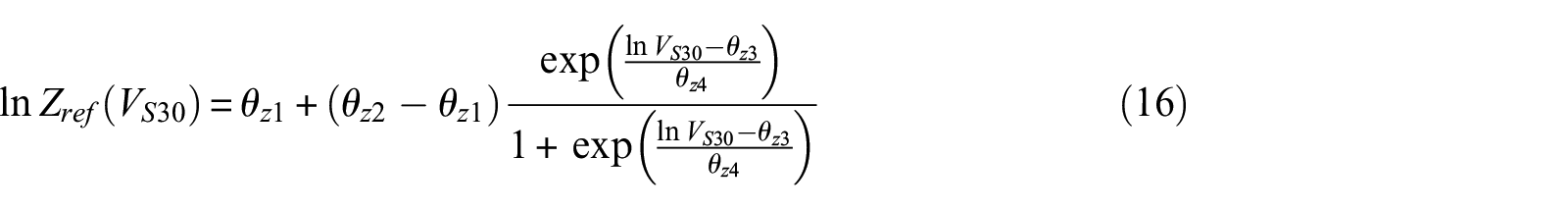
where the regional coefficients θ_z₁ through θ_z₄ are different for CASC, JP, NZ, and TW. Basin depths are not available for all subduction regions or for all recording sites within a region. Although both Z_1.0 and Z_2.5 are available for CASC, the values of Z_1.0 are typically associated with the depth to the relatively shallow high shear-wave velocity horizon at the quaternary–tertiary boundary (Stephenson et al., 2019) and is not a good representation of the deeper basin structure that amplifies intermediate-to-long period ground motion (Chang et al., 2014; Frankel et al., 2009). Both basin depths are also available for JP, but we selected Z_2.5 to be consistent with the depth parameter used by Si et al. (2022) in their basin-response term and the relatively deep basin depths that Morikawa and Fujiwara (2013) found gave the smallest standard deviations at T > 0.3 s when a basin-response term was included in their GMM. Only Z_1.0 is available for NZ and TW and no basin depths are available for AK, CAM, and SA. For regions where basin depths are available, the basin-response term is defined as a function of the difference between the observed and a reference basin depth defined by the regional relationship between basin depth and site velocity given by Equation 16. This is done to minimize the impact of the correlation between basin depth and site velocity in the regression.

Figure 3 plots V_S₃₀ versus Z_1.0 or Z_2.5 for JP, NZ, and TW together with the predictions from Equation 16. Figure 4 shows a plot of V_S₃₀ versus Z_2.5 for CASC. For sites in CASC, we distinguish between non-basin sites, for which the basin-response term is zero, and sites located within the Everett, Georgia, North Portland, Seattle, Tacoma, and Tualatin basins (Kuehn et al., 2020a). In this latter figure, the sites inside the Seattle basin are found to have basin depths of Z_2.5≈ 7000 m independent of the value of V_S₃₀. 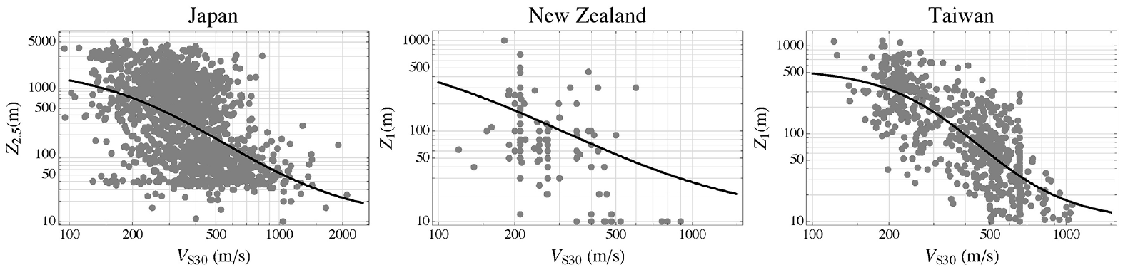If these sites were included in the regression for Equation 16, it would bias the slope of the $\ln Z_{ref}$ and $δ_{\ln Z}$ terms. To avoid this bias, we use a constant basin-amplification term (θ_11,SEA) for sites located inside the Seattle basin.

Figure 3.

Scaling of (left) Z_2.5 versus V_S₃₀ for Japan, (middle) Z_1.0 versus V_S₃₀ for New Zealand, and (right) Z_1.0 versus V_S₃₀ for Taiwan compared to the fitted models.

Figure 4.

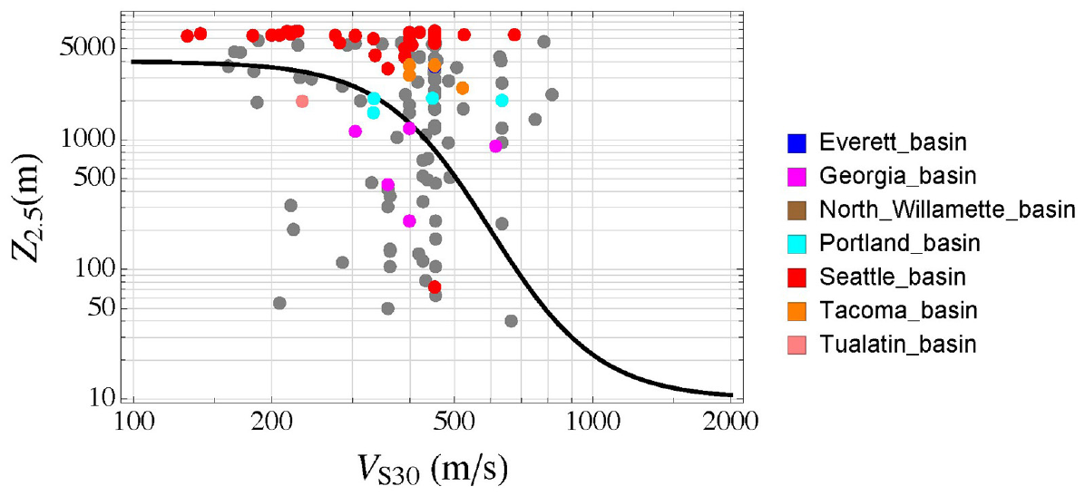
Scaling of Z_2.5 versus V_S₃₀ for Cascadia showing values of Z_2.5 for the separate basins in the region compared to the fitted model for all of the basins except for the Seattle basin (red solid circles) that was assigned a constant depth of 7000 m.

Geographic regionalization

As indicated in previous sections of this article, we account for regional differences in the constants θ_1,if and θ_1,slab; the linear site-response coefficient θ₇; the anelastic attenuation coefficients θ_6,x1, θ_6,x2, θ_6,x3, θ_6,1, θ_6,2, and θ_6,3; and the basin-response coefficients θ_z₁, θ_z₂, θ_z₃, and θ_z₄ (see Table 2). Regional differences in ground-motion scaling are expected as a result of differences in tectonic and geological conditions. In particular, regional differences in the anelastic attenuation coefficients are expected to be related to differences in the seismological quality factor Q, and regional differences in the linear site-response and basin-response terms are expected to be related to differences in the average shear-wave velocity profile. In addition, differences in the average stress drop can translate to differences in the constants at short periods. Although basin response is also regionalized, because this term is fit to the within-event residuals after the GMM is developed, it is not part of the regionalization included in the regression. There are only enough data to estimate regional basin-response terms and their epistemic standard deviations for CASC, JP, NZ, and TW and not for a global model plus these regional adjustments.

In the Bayesian regression, the regionalized coefficients are modeled as regional random effects (Stafford, 2014) according to the following equation:

{\vec{θ}}_{reg} = μ_{θ} + δ {\vec{θ}}_{reg}

(17)

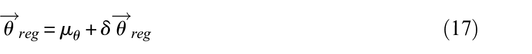
where µ_θ is the global coefficient and $δ {\vec{θ}}_{reg}$ is the regional adjustment factor. The subscript reg has been dropped from the regional coefficients throughout this article for simplicity in nomenclature. One can refer to Table 3 for those coefficients that are regionalized. The regional adjustments are joint normally distributed with mean zero and marginal standard deviation ψ_θ. For further details, see Chapter 4 of the study by Kuehn et al. (2020a) and the Supplemental material to the article.

Past studies have found that the small-magnitude short-period CASC intraslab ground motions are significantly lower compared to intraslab events from other regions (Abrahamson et al., 2016, 2018; Atkinson, 1997; Atkinson and Boore, 2003). Although we have confirmed this result, we also found that the ground motions from the two largest intraslab events in CASC are comparable to, although somewhat lower than, our global model. We did not want to bias the regional CASC constant θ_1,slab toward low values based on ground motion data from these smaller earthquakes yet there are too few of them to define a CASC-specific MSR. Therefore, we used only the two largest events, the M 6.8 Nisqually and the M 6.55 Ferndale earthquakes, in the random effects regression to derive the regional CASC constant. For the other 10 CASC intraslab events, we centered the ground motions from each event using an event-specific constant so they could be used to estimate regional linear site-response and anelastic-attenuation coefficients without impacting the regional intraslab constant.

We also found that the within-event standard deviation ϕ was smaller for those regions with a basin-response term. This was not the case for the between-event standard deviation τ that was not regionalized. We also evaluated whether the standard deviations were dependent on magnitude, distance, and subduction type (i.e. interface and intraslab), but no significant biases or trends were found due to limited data and a significant overlap of their posterior distributions. However, we did find and included a strong regional dependence of epistemic uncertainty. Additional details are available in the study by Kuehn et al. (2020a).

Regionalization of breakpoint magnitude

It is clear from modern empirical subduction interface GMMs (Abrahamson et al., 2016, 2018; Campbell et al., 2022; Morikawa and Fujiwara, 2013; Zhao et al., 2016b) and other literature reviews (Campbell, 2020; Stewart et al., 2013) that there is a magnitude at which the MSR of ground-motions from subduction interface earthquakes must become smaller. In KBCG20, this magnitude is referred to as breakpoint magnitude (M_B) after the study by Campbell (2020). The values of M_B depend on the geometry, seismogenic characteristics, and age of the subduction zone. We base the values of the breakpoint magnitude used in KBCG20 on the studies of Ji and Archuleta (2018) for intraslab events (M_B,slab) and Campbell (2020) for interface events (M_B,if). For more information, we refer the reader to these studies and Section 8.2 of the study by Kuehn et al. (2020a). The suggested values of M_B for the seven subduction zones and related subregions within these subduction zones are listed in Table 5.

Model estimation

The model parameters estimated in the Bayesian regression are the global coefficients $\vec{θ}$ , the aleatory standard deviations ϕ and τ (corresponding to within-event and between-event variability, respectively), the event terms δB, and the regional adjustment terms $δ \vec{θ}$ together with their standard deviations and correlation coefficients. The model parameters are estimated using Bayesian inference. In Bayesian inference, the posterior distribution of a model parameter is proportional to its prior distribution times its likelihood. Kruschke (2015) and Spiegelhalter and Rice (2009) provide an introduction to Bayesian inference and Kuehn et al. (2020b), Ordaz et al. (1994), Stafford (2019), and Wang and Takada (2009) provide examples of its application in GMM development.

Posterior distributions

The posterior distributions of the model parameters are estimated from Markov Chain Monte Carlo (MCMC) sampling using the Bayesian computer platform Stan (Carpenter et al., 2017). These posterior distributions are then used to calculate summary statistics such as the mean, median, fractiles and correlation coefficients of the coefficients, predicted values, and standard deviations. In total, we generate 800 samples from the posterior distribution. In Equation 1, the recording level of the GMM is modeled as a normal distribution with mean µ and within-event standard deviation ϕ, which means that the ground-motion parameter of interest Y is distributed according to a lognormal distribution. In a forward application of the model, this is how the model should be used even though the fit is done assuming a Student’s t-distribution as discussed next.

During exploratory regressions, we observed several apparent outlier recordings. Including such outliers can lead to a biased estimate of the median prediction and an increased estimate of the standard deviations. To mitigate this issue, we performed a Bayesian robust regression. Instead of modeling the within-event variability with a normal distribution as is traditionally the case, a Student’s t-distribution is used (Gelman and Hill, 2006; Kruschke, 2015). Compared to the normal distribution, the Student’s t-distribution has wider tails, which makes it less susceptible to outliers. For more details, see Chapter 5 in the study by Kuehn et al. (2020a) and the Supplemental material to this article.

To ensure a smooth predicted response spectrum, we smoothed the means of the model coefficients and aleatory standard deviations (i.e. the mean of the 800 posterior samples for each model parameter) using a Gaussian process (GP) regression (Rasmussen and Williams, 2006) with a squared exponential covariance function. For more details see Section 4.3 in the study by Kuehn et al. (2020a) and the Supplemental material to the article. The regional standard deviations are not smoothed because they do not affect the predicted median spectrum. For the same reason, the parameters of the correlation matrix of the regional coefficients are not smoothed. We re-centered the posterior distribution of each coefficient by subtracting its smoothed value from its distribution mean and adding this difference to each posterior value. Not only does this retain the range of values in the original posterior distribution, it also retains the correlation between the posterior distributions of the coefficients.

Prior distributions

We classify the prior distributions of the regression coefficients and the other model parameters as being a mix of weakly informative and informative depending on the available data. For those regression coefficients that are not well constrained by data, it is important to define informative prior distributions using other types of information (e.g. physical constraints or physics-based ground-motion simulations) for the results to be meaningful. For other model parameters, a weakly informative prior distribution is used to down-weight ranges of the parameter space that can be ruled out a priori. Although the term weakly informative is not well defined, it is usually interpreted to mean a probability distribution that is not very wide. Stafford (2019) suggests defining the prior distributions based on previous GMMs, which can help to stabilize regression results and lead to more reasonable predicted values (Kowsari et al., 2020; Kuehn and Scherbaum, 2016). However, because most GMMs do not report the full distributions of their coefficients, this information is generally not available. Furthermore, there is considerable overlap between the NGA-Sub database and data sets used in previous GMMs, which means that prior distributions based on published models might double-count some data.

We used informative prior distributions for the MSR coefficients θ_4,if and θ_4,slab for small events and θ₅ for large events, as well as for the coefficients θ_nft,₁ and θ_nft,₂ of the near-fault saturation term. The prior distributions for the other regression coefficients are described in Section 4.1.8 of the study by Kuehn et al. (2020a) and in the Supplemental material to the article. The prior distribution of θ₅ needs to be informative because there are not many events to empirically constrain it. Therefore, we base its prior distribution on results of the simulation-based GMMs of Atkinson and Macias (2009) and Gregor et al. (2002). The effective large-magnitude MSRs of these two models are shown in Figure 5. For comparison, we also plot the MSR estimated by Ghofrani and Atkinson (2014) from M > 7.0 empirical interface earthquakes in JP, although we note these authors found that their MSR at long periods was not statistically significant. To enforce magnitude saturation, but not allow oversaturation, of ground motions at large magnitudes and short distances, we constrain θ₅ to be positive and smaller than the value of θ_4,if for small-event MSRs. The standard deviation of the prior distribution is set to 0.2, corresponding to the range of MSRs across different periods, resulting in the following prior distribution for θ₅:

θ_{5} ~ N (0, 0.2) T (0, θ_{4, if})

(18)

where T(a,b) indicates a truncated normal distribution with lower limit a and upper limit b.

Figure 5.

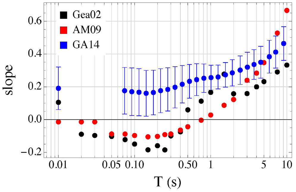
Large-magnitude scaling rates (MSRs) for selected GMMs used to set prior values in KBCG20.

The prior distributions of the MSR at magnitudes below the breakpoint magnitude are defined by the equations:

θ_{4, if} ~ N (1, 0.5) T (0, \infty)

(19)

θ_{4, slab} N (1, 0.5) T (0, \infty)

(20)

These prior distributions are informed by the physics-based simulations for intraslab events by Ji and Archuleta (2018). We performed a simple regression on the simulated ground motions and found the estimated MSR to be approximately one across all periods. Since the simulated data range is rather limited, we used the regression results as guidance to impart a wider standard deviation on the prior distribution based on the regression. The GMMs of Gregor et al. (2002) and Atkinson and Macias (2009) are valid for M > 7.5 and cannot be used to determine a prior estimate of the MSR at small magnitudes. However, we note that Campbell et al. (2022) empirically found an MSR of approximately 1 at magnitudes below the breakpoint magnitude for PGA using data from Japanese interface events.

Another parameter that needs to be constrained with an informative prior distribution is the near-fault or “pseudo-depth” term h(M) that controls the near-fault distance scaling of the GMM. This term is difficult to constrain empirically because of the limited number of recordings at short distances. We set the prior distributions of the two coefficients θ_nft,₁ and θ_nft,₂ that define this term based on the finite-fault terms in the studies by Abrahamson et al. (2016) and Parker et al. (2022). The latter study uses ground-motion simulations from the finite-fault stochastic simulation program EXSIM (Motazedian and Atkinson, 2005) to constrain the magnitude-scaling of h(M). To set the prior distribution for the finite-fault term in KBCG20, we require that the average of the prior distributions at M 6.0 and M 9.0 falls between those predicted by the Abrahamson et al. (2016) and Parker et al. (2022) GMMs. The standard deviations are set such that h(M = 9.0)_95% = 33, where h(M = 9.0)_95% is the 95% fractile of the h(M) distribution at M 9. This leads to the following prior distributions for the two coefficients controlling h(M):

θ_{nft, 1} ~ N (0.875, 0.02)

(21)

θ_{nft, 2} ~ N (0.201, 0.005)

(22)

Figure 6 shows the finite-fault terms predicted by the Abrahamson et al. (2016) and Parker et al. (2022) GMMs and the resulting prior distribution for h(M) and its 5% and 95% fractiles.

Figure 6.

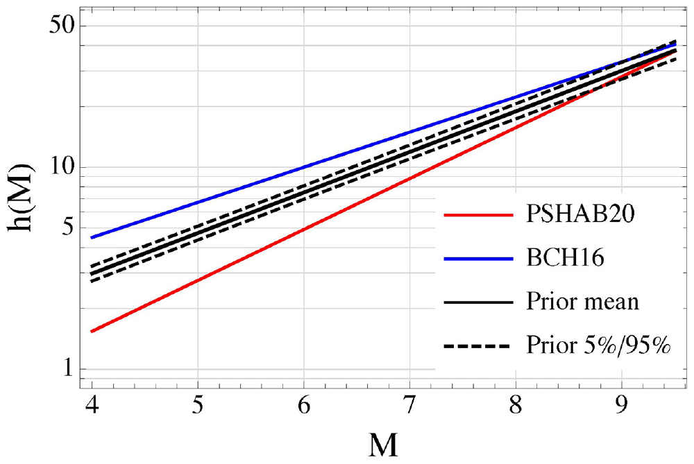
Comparison of the prior distribution of the near-fault term h(M) from KBCG20 (labeled Prior) and the modeled values of h(M) from two other studies used to inform these priors.

The prior distributions for the regional standard deviations are exponentially distributed. The rate parameters of the exponential distributions are chosen such that large deviations from the global model are penalized, consistent with that proposed by Simpson et al. (2017). This approach is akin to Occam’s razor, in which the simpler model is the global model and deviations from the global model are only modeled if there is a strong regional signal in the data. Since the number of regions is small, the estimate of the regional standard deviations can be quite noisy, which means it is important to set reasonable prior distributions for these parameters (Kuehn et al., 2020a).

Results

Regional coefficients

All of the mean model coefficients and their posterior distributions are provided in the Supplemental material to the article. Herein, we briefly summarize the results of the Bayesian regression analyses with respect to regional differences, since this is one of the unique features of KBCG20 compared to previous subduction GMMs. A more comprehensive evaluation of the other coefficients is available in Section 4.2.3 of the study by Kuehn et al. (2020a) and the Supplemental material to the article. Figure 7 shows the values of the regional adjustment values of the interface constant (δθ_1,if), the intraslab constant (δθ_1,slab), the linear site-response coefficient (δθ₇), and the anelastic-attenuation coefficient (δθ_6,2). We only show δθ_6,2 because this coefficient is used in the anelastic-attenuation terms of all regions as indicated in Equation 14.

Figure 7.

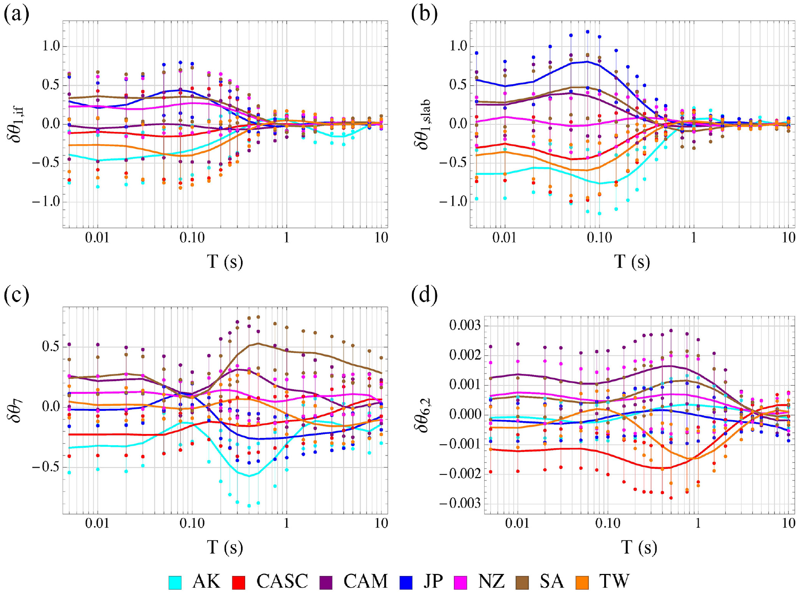
Regional regression adjustment coefficients for the (a) interface constant, (b) intraslab constant, (c) linear site-amplification coefficient, and (d) anelastic attenuation coefficient.

Figure 7 indicates that regional differences in the coefficients can be relatively large, especially at short periods. Differences at long periods are mainly restricted to linear site-response scaling. As seen in Figure 7a, the regional adjustment for the CASC interface constant is slightly negative even though there are no CASC interface events in the database. The reason for this is that the regional adjustment coefficients are modeled as correlated between interface and intraslab events and the regional adjustment of the intraslab constant is negative. This leads to a negative interface constant adjustment for CASC.

Adjustment to AK regional coefficients

The database for the NGA-Sub project was finalized on 22 April 2019 (Bozorgnia and Stewart, 2020). The GMM presented in the study by Kuehn et al. (2020a) was developed using this database. Some changes were made to the database between this date and its final publication that we reviewed to determine which aspects of our model required modification. The modifications included values of V_S₃₀ for some of the recording stations in JP and SA and values of the distance metrics in AK (Mazzoni et al., 2022). Preliminary analyses showed that changes in the predicted values due to differences in V_S₃₀ were small and could be neglected, but that changes in the predicted values due to differences in the distance metrics in AK were non-negligible. Therefore, we decided to refit the Kuehn et al. (2020a) model based on the updated AK distances. To avoid computational complexities, we only refit the AK regional adjustment coefficients to avoid having to refit the entire GMM.

In the refitting process, we fixed the global coefficients to their estimated mean values and estimated the new regionalized AK adjustment constant, site-response coefficient, and anelastic-attenuation coefficient using the revised database. The outcome of this process was a set of new posterior samples of these regional coefficients. We then calculated the mean of the posterior samples and re-centered the posterior distribution obtained from the first fit to be centered around the mean value obtained from the refitting process. In this way, we keep the original posterior range and correlations. The resulting value of the kth posterior sample for coefficient i was obtained from the equation:

θ_{i, k} (AK, refit) = θ_{i, k} (AK, origfit) - μ_{i, origfit} + μ_{i, refit}

(23)

where i is either the adjustment constant for interface events, the adjustment constant for intraslab events, the anelastic-attenuation coefficient, or the site-response coefficient, k is an index representing the 800 posterior samples, µ_i,_origfit is the mean regional coefficient from the original fit, and µ_i,_refit is the mean regional coefficient from the updated fit. This refitting process did not change the coefficients for the other subduction regions or the global model.

Aleatory variability

The total aleatory variance is calculated from the equation $σ^{2} = ϕ^{2} + τ^{2}$ . We do not account for any systematic difference in site terms because the limited azimuths of many of the recordings means that anelastic attenuation could be inadvertently mapped into site effects which would bias the standard deviations. We developed the model under the assumption that the values of τ and ϕ are the same for all subduction regions, except for the smaller value of ϕ for long-period PSA for those regions with basin-response terms. Due to a very different number of events and recordings in the different regions (see Table 2), this is a reasonable assumption as it would be difficult to obtain a reliable estimate of between-event and within-event variability for regions such as CASC or CAM where data are sparse. Figure 8 shows a plot versus period of both the original and smoothed mean values from the posterior distribution of the within-event standard deviations ϕ, the between-event standard deviations τ, and the total standard deviations σ. The uncertainty in the standard deviations is shown as the 5% and 95% fractiles of the posterior distribution.

Figure 8.

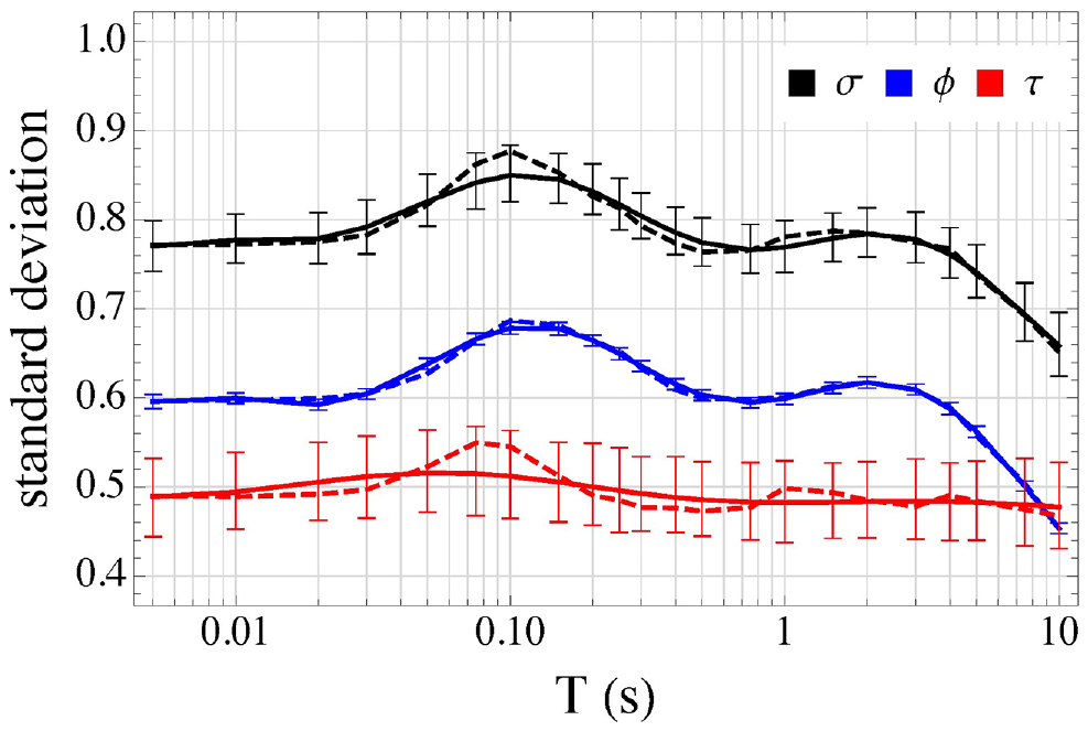
Mean original (dashed lines) and smoothed (solid lines) aleatory between-event standard deviation τ, within-event standard deviation ϕ, total standard deviation σ, and 5% and 95% fractiles (vertical lines) versus period calculated from the posterior distributions.

Model evaluation

As part of the evaluation process, we plot residuals for a limited number of ground-motion parameters and predictor variables as an example of the model validation we performed. Other residual plots are available in the study by Kuehn et al. (2020a) and at https://github.com/nikuehn/KBCG20. Figure 9 plots event terms (between-event residuals) against magnitude for T = 0.2 s and T = 3 s. Figure 10 plots within-event residuals for the same two periods against R_RUP, indicating that attenuation is not dependent on subduction type. Overall, the residuals do not show any significant biases or trends with respect to the predictor variables that would indicate an issue with the GMM.

Figure 9.

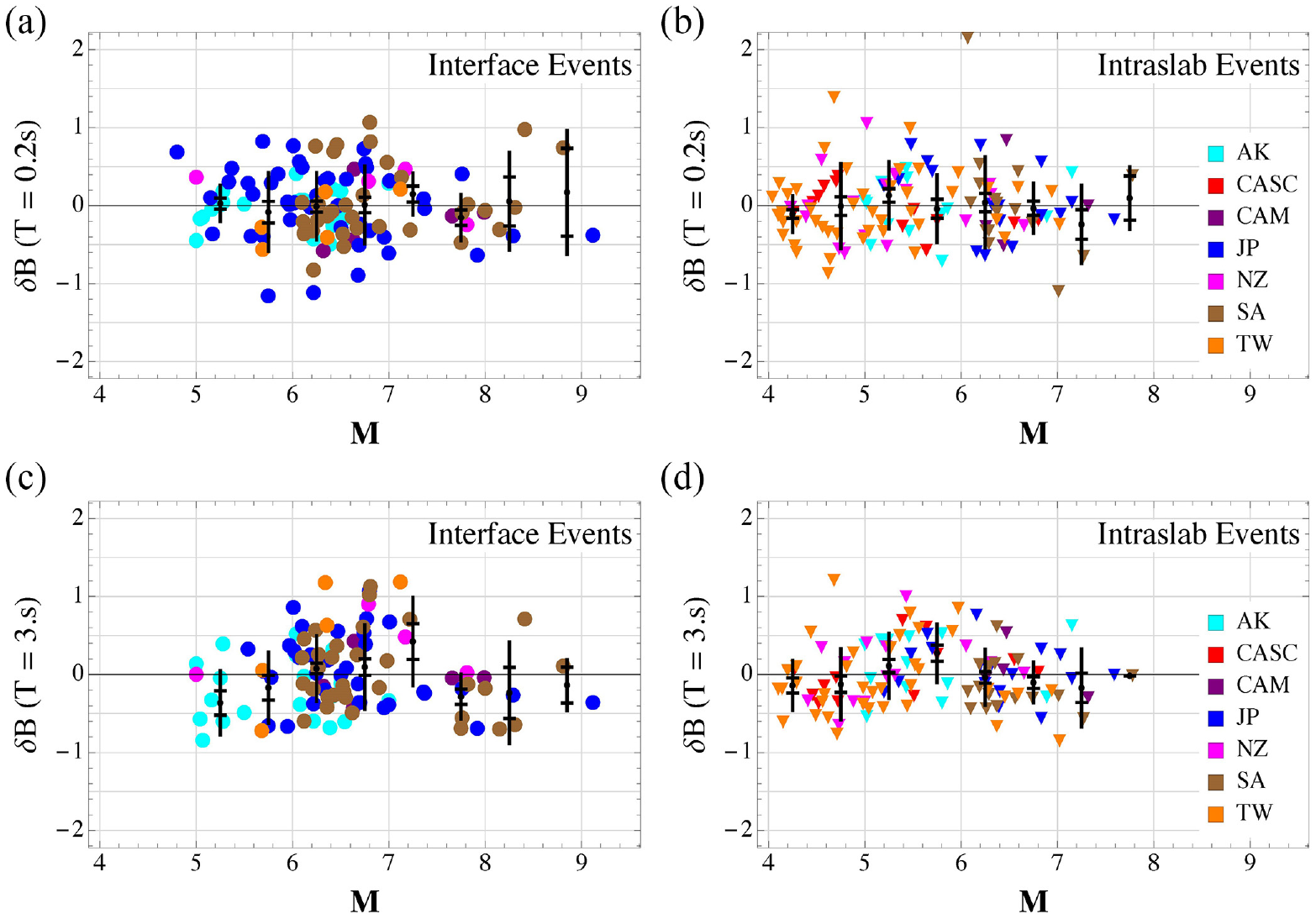
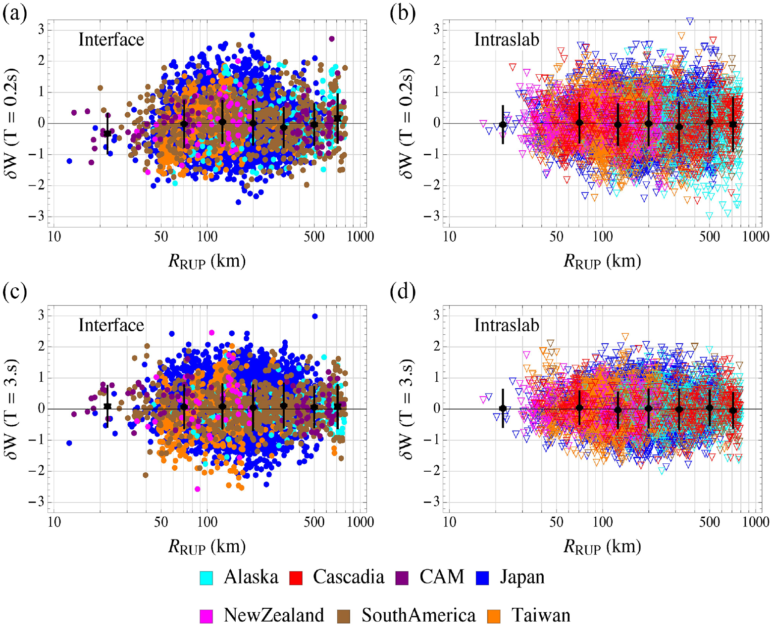
Event terms versus magnitude (M) of PSA at T = 0.2 and 3.0 s for (a and c) interface events and (b and d) intraslab events.

Figure 10.

Within-event residuals of (a) interface events for T = 0.2 s, (b) intraslab events for T = 0.2 s, (c) interface events for T = 1 s, and (d) intraslab events for T = 1 s.

Example model predictions

Figure 11 plots predicted response spectra by region for interface events at M 6 and M 9 and intraslab events at M 5 and M 8. For regions with different subregions due to differences in breakpoint magnitude, we show only one subregion to avoid making the plot too cluttered. This figure shows that the regional differences in predicted values are larger at short periods than at long periods, which is consistent with the larger differences in the regional coefficients at shorter periods seen in Figure 7. The regional differences also become more pronounced at larger magnitudes. This is due to differences in breakpoint magnitude (see Table 5). Subduction zones with a larger value of M_B have the potential to generate larger ground motions at large magnitudes. This is also seen in Figure 12 that shows the MSR of PGA for the different subduction regions and, if modeled, values of M_B for different subregions within these regions. It is impractical to compare our median predicted values and standard deviations for the global and seven regional GMMs with existing subduction models in this article. Instead, the reader is referred to comparisons in the studies by Gregor et al. (2022) and Kuehn et al. (2020a).

Figure 11.

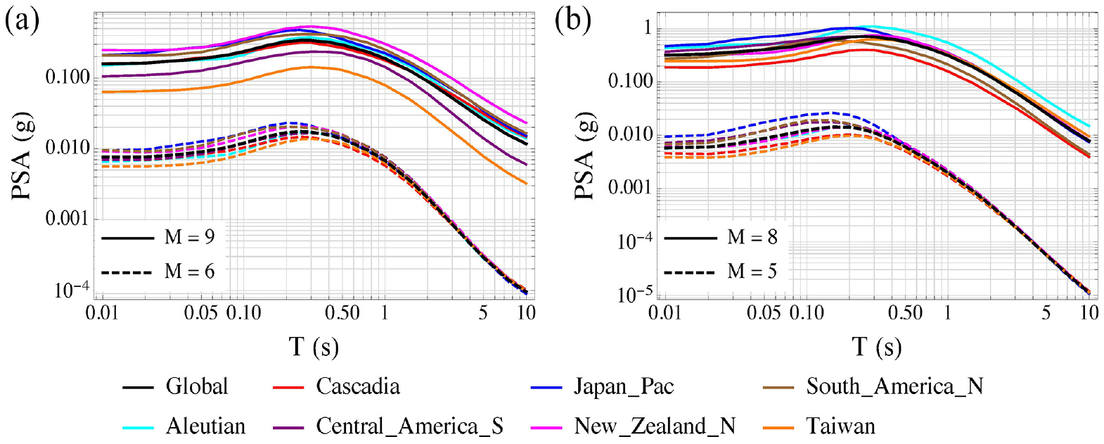
Example spectra for different subduction regions and subregions for (a) interface events with Z_TOR = 10 km and (b) intraslab events with Z_TOR = 50 km.

Figure 12.

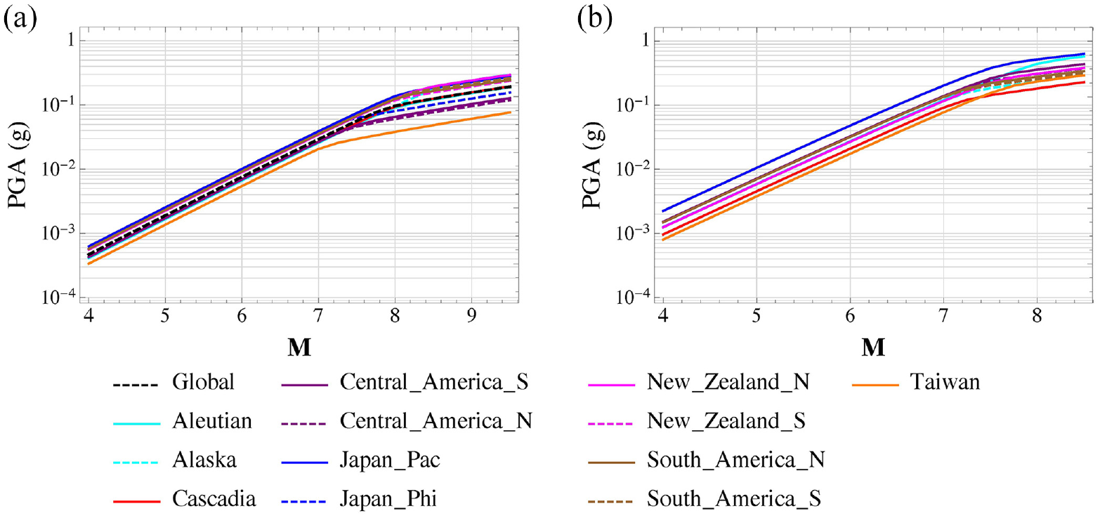
Magnitude scaling of PGA for (a) interface events with Z_TOR = 10 km and (b) intraslab events with Z_TOR = 50 km.

Epistemic uncertainty

The model parameters are estimated from a finite set of data. As a result, they inherently contain epistemic uncertainty, also referred to as within-model uncertainty. This uncertainty translates into uncertainty in the median predictions. It is important to be able to estimate this uncertainty because for some event scenarios the between-model uncertainty from a logic-tree of alternative GMMs can be small compared to within-model uncertainty. Examples of within-model uncertainty models are given by Al Atik and Youngs (2014), Lanzano et al. (2019), and Kotha et al. (2020).

In a Bayesian regression, epistemic uncertainty is quantified by a posterior distribution of model parameters. In KBCG20, the posterior distribution of each regression parameter consists of 800 samples using the MCMC methodology. Thus, there are 800 sets of regression coefficients, aleatory standard deviations, and coefficient correlations, which can be used to create 800 samples of the median predicted values and standard deviations of a given scenario event from which the mean, standard deviation, and fractiles of the median prediction can be calculated.

Figure 13a gives an example of the epistemic distribution of the predicted PSA spectrum for a particular scenario in JP. The results are in the form of a histogram of the median estimates of PSA at T = 0.01 s calculated from the 800 sets of coefficients from the posterior distribution. The median prediction is also shown for comparison. Figure 13b shows the mean MSR of PSA at T = 0.01 s for the scenario event calculated from the mean coefficients along with 10 randomly selected samples from the posterior distribution. Also shown are the 5% and 95% fractiles of the epistemic distribution for each magnitude. The 5% and 95% fractiles are calculated independently for each magnitude, meaning that different sets of sampled coefficients can contribute to the highest and lowest predicted values at each of the magnitudes. We highlight the predicted value from one particular sample in Figure 13b that has a steeper MSR than the mean to demonstrate the importance of within-model uncertainty in estimating ground motion. It also serves as a reminder that epistemic uncertainty permeates all aspects of the model (e.g. magnitude scaling, distance scaling, and site response).

Figure 13.

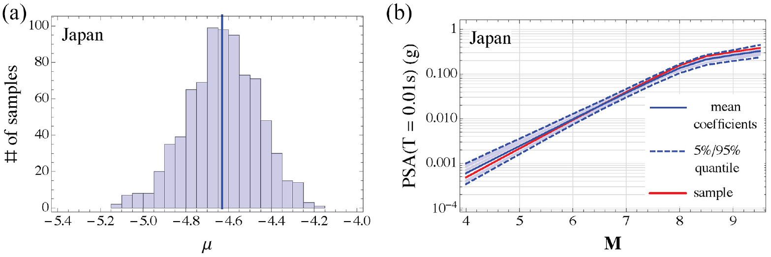
Examples of epistemic uncertainty showing (a) a histogram of 800 calculated median predictions of PSA at T = 0.01 s for Japan (JP), M = 6, R_RUP = 100 km, V_S₃₀ = 400 m/s, Z_TOR = 10 km, F_S = 0, and F_X = 0, where the vertical line is the median prediction from the mean coefficients and (b) scaling of PSA versus magnitude at T = 0.01 s for the mean coefficients (sold blue line), 90% confidence limits of the mean coefficients (dashed blue lines), and 10 individual samples (light blue lines) taken from the posterior distribution.

It is especially important to account for epistemic uncertainty in partially nonergodic models so as not to underestimate the seismic hazard (Abrahamson et al., 2019). The regional adjustment terms are calculated from a relatively small number of recordings and are associated with more epistemic uncertainty than the global model in which all data are pooled. This is particularly important for regions with a small number of recordings such as CASC. 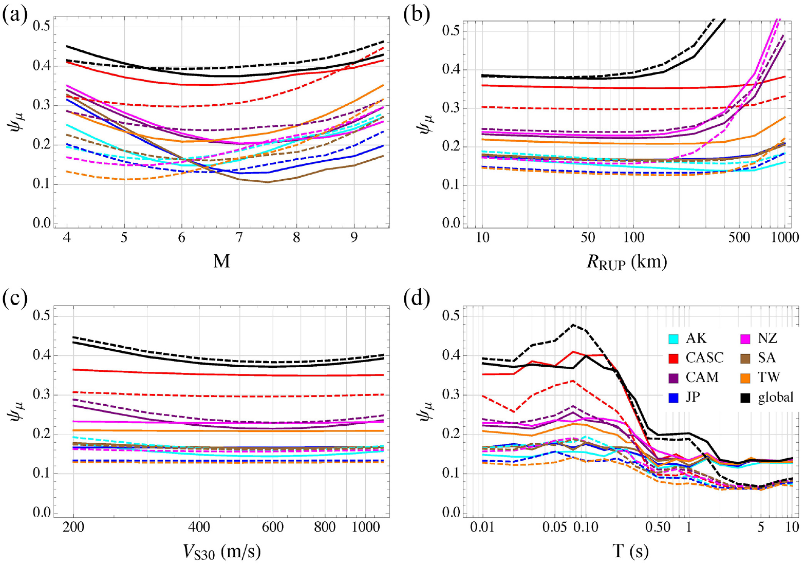This is demonstrated in Figure 14 in which we plot the epistemic standard deviation of the median predicted value of PGA (ψ_µ) from the global model and the seven defined regions versus M, R_RUP, V_S₃₀, and T. This figure shows that epistemic uncertainty is relatively small for regions with a large number of recordings (e.g. JP and SA) and relatively large for regions with a small number of recordings (e.g. CASC and CAM).

Figure 14.

Epistemic standard deviations (ψ_µ) associated with median predictions of ground motion: (a) PGA versus magnitude (M), (b) PGA versus rupture distance R_RUP, (c) PGA versus site velocity V_S₃₀, and (d) PSA versus period T.

Figure 14d shows that there are larger regional differences between the values of µ at short periods than at long periods. This is because the longer-period coefficients are better constrained in the regression (see Figure 7). We also show values of µ for the global model, which are applicable when KBCG20 is applied to a new region. To calculate median predictions for the global model, we sample regional adjustment terms from their joint distribution and add the sampled adjustment terms to the coefficients from the posterior distribution as described in the study by Gelman and Hill (2006). This shows that the CASC values of µ are closer to the values of the global model for interface events than for intraslab events, consistent with the fact that there are no CASC interface events in the database.

Table 6 illustrates the effect of regionalization of epistemic uncertainty on the predicted value of PGA. Note that, although the value of ϕ in this table is the same for all regions, it is smaller at longer periods for those regions that include a basin-response term (CASC, JP, NZ, TW). Table 6 compares the values of ϕ, τ, and total aleatory standard deviation σ and the regional epistemic standard deviations ψ_µ to the standard deviations from a nonregionalized model (i.e. a model that includes only event terms). The nonregionalized model uses the same functional form and Bayesian regression methodology as KBCG20 except that none of the coefficients are regionalized. For the nonregionalized model, the coefficients are determined using all recordings in the database, which leads to a very small value of epistemic uncertainty. However, this small value of epistemic uncertainty is offset by larger values of ϕ and τ. The total predictive variability, which sums the aleatory and epistemic variances and describes the full range of all possible ground motions, is calculated as $σ_{pred}^{2} = τ^{2} + ϕ^{2} + ψ_{μ}^{2}$ . This shows that the total predicted variability of the ground motion estimated from the regionalized global model when applied to a new region is very close to the total variability of the nonregionalized model, except that the epistemic uncertainty is a larger component of the total variability. This is an example of the trade-off between epistemic uncertainty and aleatory variability. The value of aleatory variability is reduced in the regionalized model, but there is a penalty for this reduction in the form of greater uncertainty for regions with less data. However, this trade-off is beneficiary for regions with a relatively large amount of data, as indicated by the reduction in the value of $σ_{pred}$ compared to the nonregionalized model.

Table 6.

Standard deviations of aleatory variability (ϕ, τ and σ), epistemic uncertainty (ψ_µ), and total predictive variability (σ_pred) for the different regional models compared to a (nonregionalized) global model

Region	ϕ	τ	σ	ψ_µ	σ_pred
Alaska (AK)	0.5958	0.4887	0.7706	0.1613	0.7873
Cascadia (CASC)	0.5958	0.4887	0.7706	0.3699	0.8548
Central America and Mexico (CAM)	0.5958	0.4887	0.7706	0.2205	0.8015
Japan (JP)	0.5958	0.4887	0.7706	0.1351	0.7823
New Zealand (NZ)	0.5958	0.4887	0.7706	0.2169	0.8005
South America (SA)	0.5958	0.4887	0.7706	0.1254	0.7807
Taiwan (TW)	0.5958	0.4887	0.7706	0.2034	0.7970
Global (regionalized)	0.5958	0.4887	0.7706	0.3625	0.8516
Nonregionalized	0.6265	0.5966	0.8651	0.0155	0.8652

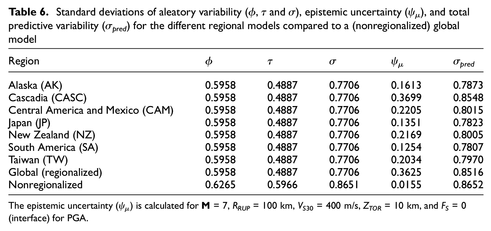
The epistemic uncertainty (ψ_µ) is calculated for M = 7, R_RUP = 100 km, V_S₃₀ = 400 m/s, Z_TOR = 10 km, and F_S = 0 (interface) for PGA.

Engineering application

We consider KBCG20 to be generally applicable for estimating ground motions for the following range of parameters (Kuehn et al., 2020a).

General applications and global model

Ground-motion parameters: PGA (g), PGV (cm/s), PSA (g) at T = 0.01–10 s

Magnitudes: M ≥ 5.0, M≤ 8.5 (intraslab events), M≤ 9.5 (interface events)

Breakpoint magnitudes: M_B = 7.6 (intraslab events), M_B = 7.9 (interface events)

Source depths: Z_TOR≤ 50 km (interface events), Z_TOR≤ 200 km (intraslab events)

Rupture distances: 10 ≤R_RUP≤ 800 km

Anelastic attenuation: Forearc (e.g. coefficient θ_6,2)

Site velocity: 100 ≤V_S₃₀≤ 1000 m/s

Basin or sediment depths: Not applicable (see regional applicability)

Regional applications

Breakpoint magnitudes: See Table 5.

Source depths: Z_TOR≤ 150 km for intraslab events in Colombia (SA)

Anelastic attenuation: Forearc (AK, CAM, CASC, NZ, JP, SA, TW), Backarc (AK, JP, NZ)

Basin (sediment) depths: Z_2.5≤ 10 km (CASC, JP), Z_1.0≤ 2.2 km (NZ, TW)

The user should be aware that the epistemic standard deviation can increase (possibly considerably) if one or more of the predictor variables are near or beyond the limit of their observed values for the region of interest.

The total value of the aleatory component of variance is $σ^{2} = ϕ^{2} + τ^{2}$ , which is the value that should be used in the hazard integral to account for aleatory variability. The most comprehensive estimate of epistemic variance is obtained from the full posterior distribution from the Bayesian regression and should be modeled using a logic tree. However, if one is only interested in the mean hazard and not its fractiles, but still wants to include epistemic uncertainty in the hazard analysis, the value of total predictive variability $σ_{pred}^{2} = ϕ^{2} + τ^{2} + ψ_{μ}^{2}$ can be used in the hazard integral, thus avoiding the necessity of using a logic tree. To facilitate the use of within-model uncertainty in engineering analyses, and particularly in PSHA, we pre-calculated the epistemic within-model standard deviations (ψ_µ) associated with the median predictions of interface and intraslab events for different magnitude and distance scenarios, holding the other predictor variables constant. These values are available at https://github.com/nikuehn/KBCG20 and can be used as a simplified version of epistemic uncertainty based on the observation that the value of ψ_µ depends only marginally on the values of Z_TOR, V_S₃₀, Z_1.0, and Z_2.5. They also can be used to estimate magnitude- and distance-dependent scale factors to use with the median values from KBCG20 using a scaled backbone approach similar to that proposed in the study by Atkinson et al. (2014).

KBCG20 can be used to estimate ground motions for seven different subduction-zone regions. However, there are other subduction zones located throughout the world for which GMMs might be needed to perform a PSHA or deterministic seismic hazard analysis (e.g. the 79 subduction zones identified in the studies by Berryman et al., 2015 and Campbell, 2020). Some of these subduction zones might have limited or no ground-motion data. In that case the regionalized KBCG20 global model with its larger epistemic standard deviation should be used.

The epistemic uncertainty discussed above and in the Epistemic Uncertainty section of the article represents within-model uncertainty, since it only addresses uncertainty in the median estimates of the ground motion. Additional GMMs, such as those developed as part of the NGA-Sub project (Bozorgnia et al., 2022) or other published GMMs, should be used to account for between-model epistemic uncertainty similar to that recommended by Al Atik and Youngs (2014) for the NGA-West2 GMMs. The use of additional GMMs can address differences in basic assumptions, such as the functional form of the model and the database used to develop it, that are not accounted for in within-model uncertainty. The within-model uncertainty should be seen as a minimum representation of epistemic uncertainty.

An important aspect of KBCG20 is the use of regionalized breakpoint magnitudes (M_B,if for interface events and M_B,slab for intraslab events), which have a strong impact on the predicted values of ground motion at magnitudes exceeding these breakpoints. The values of breakpoint magnitude provided in this article are based on the geometry, seismogenic characteristics, and age of the subduction zone (Campbell, 2020; Ji and Archuleta, 2018) and should not be considered an inalienable parameter. KBCG20 is designed such that it is easy to replace breakpoint magnitudes in the GMM without impacting other aspects of the model, which facilitates the inclusion of epistemic uncertainty in these magnitudes for a given region or replacing them with more appropriate values for a new region (Campbell, 2020).

We did not partition the aleatory standard deviations of the within-event residuals from KBCG20 into a site term (ϕ_S_2S) and an event- and site-corrected (single-station) standard deviation (ϕ_SS) because of the relatively narrow azimuthal range of the recordings and the potential that unmodeled path effects might be mapped into the site terms. Therefore, the aleatory variability is ergodic with respect to the site model. If a single-station standard deviation is desired, we suggest that studies available in the literature be used to estimate reduction factors to apply to ϕ to estimate ϕ_SS. The majority of these single-station standard deviations are for crustal earthquakes, but some recent studies provide estimates of ϕ and ϕ_SS for subduction earthquakes in Chile (Montalva et al., 2017, 2022), JP (Campbell et al., 2022; Hassani and Atkinson, 2021; Zhao et al., 2016a, 2016b), northern South America (Arteta et al., 2021), TW (Chao et al., 2020; Phung et al., 2020), and globally (Abrahamson and Gulerce, 2022; Parker et al., 2022).

Cascadia Subduction Zone

The CASC is an example of why uncertainty in breakpoint magnitude should be considered. Campbell (2020) estimates a mean value for M_B,if of 7.7 with epistemic 5% and 95% confidence limits of 7.3 and 8.2, respectively. These values are based on a relatively narrow preferred average seismogenic interface width of 68 km estimated by Berryman et al. (2015). Campbell (2020) poses the question of whether an earthquake that originates on the wider section of the CASC interface in the Puget Sound region will exhibit a larger breakpoint magnitude. To account for this uncertainty, a larger value of M_B,if could be used for hypocenters located in the Puget Sound region and a smaller one for hypocenters originating along the narrower sections of the CASC interface. Alternatively, epistemic uncertainty could be modeled using a single set of breakpoint magnitudes regardless of hypocenter location. For example, Campbell (2020) suggests one possible set of values for M_B,if could be 7.7 (5% confidence limit), 8.0 (mean), and 8.5 (95% confidence limit) with weights of 0.185, 0.630, and 0.185, respectively. We suggest using the mean of this distribution if only a single value of M_B,if is used (see Table 5). Figure 15 shows the effect at large magnitudes of using the three-point discrete distribution of breakpoint magnitudes on the median prediction of PGA.

Figure 15.

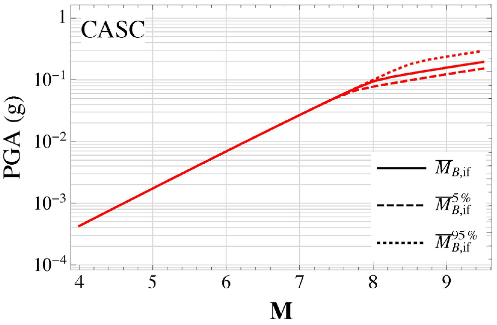
Magnitude scaling for interface events in Cascadia (CASC) using the mean breakpoint magnitude and its uncertainty according to Campbell (2020).

Another potential issue with the prediction of ground motions for CASC interface events is the lack of interface earthquakes. As a result, we assumed that anelastic attenuation for CASC interface events was the same as for CASC intraslab earthquakes consistent with the CASC model of Abrahamson et al. (2018). On the contrary, Abrahamson and Gulerce (2022) assume that CASC intraslab events have a higher rate of attenuation than interface events consistent with their global GMM and Parker et al. (2022) assume that CASC interface events have a higher rate of attenuation than intraslab events consistent with their global GMM for interface events and their CASC-specific attenuation term for intraslab events. This uncertainty is not restricted to global and regional NGA-Sub models. Zhao et al. (2016a, 2016b) found that intraslab events had a higher rate of attenuation than interface events, whereas Si et al. (2022) found both types of events to have the same rate of attenuation. These results indicate that our assumption of similar anelastic attenuation of interface and intraslab events is not unreasonable.

All of the NGA-Sub GMMs have stronger attenuation in the backarc region of CASC than that in the study by Abrahamson et al. (2016), but similar forearc attenuation at short periods as that by Abrahamson et al. (2016) and the M9 project simulations of Frankel et al. (2018). At long periods, the M9 simulations have less attenuation than all of the NGA-Sub models for reasons that are not known at this time. We conclude that there is a great deal of epistemic uncertainty associated with ground-motion attenuation in CASC that should be taken into account in a hazard analysis for this region.

Summary and conclusion

This article presents a partially nonergodic empirical GMM for subduction interface and intraslab events developed using the extensive global NGA-Sub database. The GMM is partially nonergodic in three aspects: (1) it includes an event term as a random effect; (2) it accounts for regional differences in overall amplitude, anelastic attenuation, linear site response, and basin response as random effects for subduction zones in AK, CAM, CASC, JP, NZ, SA, and TW; and (3) it accounts for regional differences in breakpoint magnitude between subregions of the seven regionalized subduction zones. In addition, there is a global model that can be used for sites outside of the defined regions or as an epistemic alternative to a regional model. Site terms are not evaluated in the GMM but can be estimated from published GMMs. Implementation guidelines are provided in the “Engineering Application” section of the article.

We recommend that our GMM be used together with other credible and appropriate GMMs for the site or region of interest to capture between-model epistemic uncertainty in a seismic hazard analysis. No single model, even if it includes within-model epistemic uncertainty as ours does, should be used to characterize seismic hazard. Our regionalized global model should be used along with its larger epistemic uncertainty when applying it to a subduction zone not characterized in this study. If some data are available for a new region, a Bayesian approach similar to that recommended by Stafford (2019) can be used to adjust the global GMM to this region.

Supplemental Material

sj-pdf-1-eqs-10.1177_87552930231180906 – Supplemental material for A regionalized partially nonergodic ground-motion model for subduction earthquakes using the NGA-Sub database

Supplemental material, sj-pdf-1-eqs-10.1177_87552930231180906 for A regionalized partially nonergodic ground-motion model for subduction earthquakes using the NGA-Sub database by Nicolas M Kuehn, Yousef Bozorgnia, Kenneth W Campbell and Nicholas Gregor in Earthquake Spectra

Footnotes

Acknowledgements

Following the tradition of all NGA research projects, the ground-motion modeling teams as well as database developers have had continuous technical interactions that resulted in a higher quality of the final products than each researcher could achieve individually. Special thanks should be given to numerous junior and senior researchers and practicing professionals who worked on various sub-tasks of the NGA-Sub research program. Their contributions, dedication, and teamwork are greatly appreciated. We also thank three reviewers for their insightful comments that helped to improve the article.

Data and resources

The GMM developed in this study has been coded in multiple computer platforms including Visual Basic in Excel, R, MATLAB, and Python available at https://www.risksciences.ucla.edu/nhr3/gmtools . The coefficients of the model as well as an implementation of the GMM in the R software environment (R Core Team, 2023) is available at https://github.com/nikuehn/KBCG20 and the to the article and can be used to estimate median predictions and between-event, within-event, and within-model standard deviations and their associated posterior distributions.

Declaration of conflicting interests

The authors declared no potential conflicts of interest with respect to the research, authorship, and/or publication of this article.

Funding

The authors disclosed receipt of the following financial support for the research, authorship, and/or publication of this article: This study was supported by FM Global, the US Geological Survey, the California Department of Transportation, and the Pacific Gas and Electric Company. This support is gratefully acknowledged. The opinions, findings, conclusions, or recommendations expressed in this publication are those of the authors and do not necessarily reflect the views of the study sponsors.

ORCID iDs

Nicolas M Kuehn

Yousef Bozorgnia

Kenneth W Campbell

Nicholas Gregor

Supplemental material

Supplemental material for this article is available online.

References

Abrahamson

Gulerce

(2022) Summary of the Abrahamson and Gulerce NGA-SUB ground-motion model for subduction earthquakes. Earthquake Spectra 38(4): 2638–2681.

Abrahamson

Gregor

Addo

(2016) BC Hydro ground motion prediction equations for subduction earthquakes. Earthquake Spectra 32(1): 23–44.

Abrahamson

Kuehn

Gulerce

Gregor

Bozorgnia

Parker

Stewart

Chiou

BS-J

Idriss

Campbell

Youngs

(2018) Update of the BC hydro subduction ground-motion model using the NGA-subduction dataset. PEER report no. 2018/02, 2 June. Berkeley, CA: Pacific Earthquake Engineering Research Center (PEER), University of California, Berkeley.

Abrahamson

Kuehn

Walling

Landwehr

(2019) Probabilistic seismic hazard analysis in California using nonergodic ground-motion models. Bulletin of the Seismological Society of America 109(4): 1235–1249.

Al Atik

Youngs

(2014) Epistemic uncertainty for NGA-West2 models. Earthquake Spectra 30(3): 1301–1318.

Anderson

Brune

(1999) Probabilistic seismic hazard analysis without the ergodic assumption. Seismological Research Letters 70(1): 19–28.

Arteta

Pajaro

Mercado

Montejo

Arcila

Abrahamson

(2021) Ground-motion model for subduction earthquakes in northern South America. Earthquake Spectra 37(4): 2419–2452.

Atkinson

(1997) Empirical ground motion relations for earthquakes in the Cascadia region. Canadian Journal of Civil Engineering 24(1): 64–77.

Atkinson

Boore

(2003) Empirical ground-motion relations for subduction-zone earthquakes and their application to Cascadia and other regions. Bulletin of the Seismological Society of America 93(4): 1703–1729.

10.

Atkinson

Boore

(2008) Erratum to “empirical ground-motion relations for subduction zone earthquakes and their application to Cascadia and other regions.” Bulletin of the Seismological Society of America 98(5): 2567–2569.

11.

Atkinson

Macias

(2009) Predicted ground motions for great interface earthquakes in the Cascadia Subduction Zone. Bulletin of the Seismological Society of America 99(3): 1552–1578.

12.

Atkinson

Bommer

Abrahamson

(2014) Alternative approaches to modeling epistemic uncertainty in ground motions in probabilistic seismic-hazard analysis. Seismological Research Letters 85(6): 1141–1144.

13.

Berryman

Wallace

Hayes

Bird

Wang

Basili

Lay

Pagani

Stein

Sagiya

Rubin

Barreintos

Kreemer

Litchfield

Stirling

Gledhill

Haller

Costa

(2015) Characterisation of subduction zones. The GEM Faulted Earth Subduction Interface Characterisation Project, Report Produced in the Context of the GEM Faulted Earth Global Component, Global Earthquake Model (GEM) Foundation, Pavia.

14.

Boore

(2010) Orientation-independent, nongeometric-mean measures of seismic intensity from two horizontal components of motion. Bulletin of the Seismological Society of America 100(4): 1830–1835.

15.

Bozorgnia

Abrahamson

Ahdi

Ancheta

Al Atik

Archuleta

Atkinson

Boore

Campbell

Chiou

BS-J

Contreras

Darragh

Derakhshan

Donahue

Gregor

Gulerce

Idriss

Kishida

Kottke

Kuehn

Kwak

Kwok

AOL

Lin

Macedo

Mazzoni

Midorikawa

Muin

Parker

Rezaeian

Silva

Stewart

Walling

Wooddell

Youngs

(2022) NGA-Subduction research program. Earthquake Spectra 38(2): 783–798.

16.

Bozorgnia

Stewart

(2020) Data resources for NGA-subduction project. PEER report no. 2020/02, 1 March. Berkeley, CA: Pacific Earthquake Engineering Research Center (PEER), University of California, Berkeley.

17.

Campbell

(2020) Proposed methodology for estimating the magnitude at which subduction megathrust ground motions and source dimensions exhibit a break in magnitude scaling: Example for 79 global subduction zones. Earthquake Spectra 36(3): 1271–1297.

18.

Campbell

Bozorgnia

(2014) NGA-West2 ground motion model for the average horizontal components of PGA, PGV, and 5% damped linear acceleration response spectra. Earthquake Spectra 30(3): 1087–1115.

19.

Campbell

Bozorgnia

Kuehn

Gregor

(2022) An evaluation of partially nonergodic PGA ground-motion models for Japanese megathrust earthquakes. Earthquake Spectra 38(4): 2611–2637.

20.

Carpenter

Gelman

Hoffman

Lee

Goodrich

Betancourt

Brubaker

Guo

Riddell

(2017) Stan: A probabilistic programming language. Journal of Statistical Software 76(1): 1–32.

21.

Chang

Frankel

Weaver

(2014) Report on workshop to incorporate basin response in the design of tall buildings in the Puget Sound region, Washington. Open-file report 2014-1196, 23 September. Seattle, WA: US Geological Survey.

22.

Chao

Chiou

BS-J

Hsu

Lin

(2020) A horizontal ground-motion model for crustal and subduction earthquakes in Taiwan. Earthquake Spectra 36(2): 463–506.

23.

Contreras

Stewart

Kishida

Darragh

Chiou

BS-J

Mazzoni

Youngs

Kuehn

Ahdi

Wooddell

Boroschek

Rojas

Ordenes

(2022) NGA-Sub source and path database. Earthquake Spectra 38(2): 799–840.

24.

Fayaz

Medalla

Torres-Rodas

Galasso

(2023) A recurrent-neural-network-based generalized ground-motion model for the Chilean subduction seismic environment. Structural Safety 100: 102282.

25.

Frankel

Stephenson

Carver

(2009) Sedimentary basin effects in Seattle, Washington: Ground-motion observations and 3D simulations. Bulletin of the Seismological Society of America 99(3): 1579–1611.

26.

Frankel

Wirth

Marafi

Vidale

Stephenson

(2018) Broadband synthetic seismograms for magnitude 9 earthquakes on the Cascadia megathrust based on 3D simulations and stochastic synthetics, Part 1: Methodology and overall results. Bulletin of the Seismological Society of America 108(5A): 2347–2369.

27.

Gelman

Hill

(2006) Data Analysis Using Regression and Multilevel/Hierarchical Models. Cambridge, MA: Cambridge University Press.

28.

Gelman

Carlin

Stern

Dunson

Vehtari

Rubin

(2013) Bayesian Data Analysis. 3rd ed. Boca Raton, FL: Chapman & Hall/CRC Press.

29.

Ghofrani

Atkinson

(2014) Ground-motion prediction equations for interface earthquakes of M7 to M9 based on empirical data from Japan. Bulletin of Earthquake Engineering 12(2): 549–571.

30.

Gregor

Addo

Abrahamson

Al Atik

Atkinson

Boore

Bozorgnia

Campbell

Chiou

BS-J

Gulerce

Hassani

Kishida

Kuehn

Mazzoni

Midorikawa

Parker

Stewart

Youngs

(2022) Comparisons of the NGA-Subduction ground motion models. Earthquake Spectra 38(4): 2580–2610.

31.

Gregor

Silva

Wong

Youngs

(2002) Ground-motion attenuation relationships for Cascadia subduction zone megathrust earthquakes based on a stochastic finite-fault model. Bulletin of the Seismological Society of America 92(5): 1923–1932.

32.

Hassani

Atkinson

(2021) Equivalent point-source ground-motion model for subduction earthquakes in Japan. Bulletin of the Seismological Society of America 111(2): 951–974.

33.

Idini

Rojas

Ruiz

Pastén

(2017) Ground motion prediction equations for the Chilean subduction zone. Bulletin of Earthquake Engineering 15: 1853–1880.

34.

Archuleta

(2018) Scaling of PGA and PGV Deduced from Numerical Simulations of Intraslab Earthquakes (Report). Santa Barbara, CA: Department of Earth Sciences, University of California, Santa Barbara.

35.

Kkallas

Papazachos

Margaris

Boore

Ventouzi

Skarlatoudis

(2018) Stochastic strong ground motion simulation of the southern Aegean Sea Benioff zone intermediate-depth earthquakes. Bulletin of the Seismological Society of America 108(2): 946–965.

36.

Kotha

Weatherill

Bindi

Cotton

(2020) A regionally-adaptable ground-motion model for shallow crustal earthquakes in Europe. Bulletin of Earthquake Engineering 18(9): 4091–4125.

37.

Kowsari

Sonnemann

Halldorsson

Hrafnkelsson

Snaebjörnsson

Jonsson

(2020) Bayesian inference of empirical ground motion models to pseudo-spectral accelerations of south Iceland seismic zone earthquakes based on informative priors. Soil Dynamics and Earthquake Engineering 132: 106075.

38.

Kruschke

(2015) Doing Bayesian Data Analysis: A Tutorial with R, JAGS, and Stan. 2nd ed. London: Academic Press.

39.

Kuehn

Scherbaum

(2016) A partially non-ergodic ground-motion prediction equation for Europe and the Middle East. Bulletin of Earthquake Engineering 14(10): 2629–2642.

40.

Kuehn

Bozorgnia

Campbell

Gregor

(2020a) Partially non-ergodic ground-motion model for subduction regions using the NGA-subduction database. PEER report no. 2020/04, 1 September. Berkeley, CA: Pacific Earthquake Engineering Research Center (PEER), University of California, Berkeley.

41.

Kuehn

Kishida

AlHamaydeh

Lavrentiadis

Bozorgnia

(2020b) A Bayesian model for truncated regression for the estimation of empirical ground-motion models. Bulletin of Earthquake Engineering 18(14): 6149–6179.

42.

Lanzano

Luzi

Pacor

Felicetta

Puglia

Sgobba

D’Amico

(2019) A revised ground-motion prediction model for shallow crustal earthquakes in Italy. Bulletin of the Seismological Society of America 109(2): 525–540.

43.

Macedo

Liu

(2022) A nonergodic ground motion model for Chile. Bulletin of the Seismological Society of America 112(5): 2542–2561.

44.

Mazzoni

Kishida

Stewart

Contreras

Darragh

Ancheta

Chiou

BS-J

Silva

Bozorgnia

(2022) Relational database used for ground-motion model development in the NGA-sub project. Earthquake Spectra 38(2): 1529–1548.

45.

Montalva

Bastías

Leyton

(2022) Strong ground motion prediction model for PGV and spectral velocity for the Chilean Subduction Zone. Bulletin of the Seismological Society of America 112(1): 348–360.

46.

Montalva

Bastías

Rodriguez-Marek

(2017) Ground-motion prediction equation for the Chilean Subduction Zone. Bulletin of the Seismological Society of America 107(2): 901–911.

47.

Morikawa

Fujiwara

(2013) A new ground motion prediction equation for Japan applicable up to M9 mega-earthquake. Journal of Disaster Research 8(5): 878–888.

48.

Motazedian

Atkinson

(2005) Stochastic finite-fault modeling based on a dynamic corner frequency. Bulletin of the Seismological Society of America 95(3): 995–1010.

49.

Ordaz

Arciniega

Singh

(1994) Bayesian attenuation regressions: An application to Mexico City. Geophysical Journal International 117(2): 335–344.

50.

Parker

Stewart

Boore

Atkinson

Hassani

(2022) NGA-Subduction global ground motion models with regional adjustment factors. Earthquake Spectra 38(1): 456–493.

51.

Petersen

Shumway

Powers

Mueller

Moschetti

Frankel

Rezaeian

McNamara

Luco

Boyd

Rukstales

Jaiswal

Thompson

Hoover

Clayton

Field

Zeng

(2020) The 2018 update of the US National Seismic Hazard Model: Overview of model and implications. Earthquake Spectra 36(1): 5–41.

52.

Phung

Loh

Chao

Abrahamson

(2020) Ground motion prediction equation for Taiwan subduction zone earthquakes. Earthquake Spectra 36(3): 1331–1358.

53.

R Core Team (2023) The R project for statistical computing. Available at: https://www.R-project.org (accessed 19 May 2023).

54.

Rasmussen

Williams

CKI

(2006) Gaussian Processes for Machine Learning. Cambridge, MA: The MIT Press.

55.

Midorikawa

Kishida

(2022) Development of NGA-Sub ground-motion prediction equation of 5%-damped pseudo-spectral acceleration based on database of subduction earthquakes in Japan. Earthquake Spectra 38(4): 2682–2706.

56.

Simpson

Rue

Riebler

Martins

Sørbye

(2017) Penalising model component complexity: A principled, practical approach to constructing priors. Statistical Science 32(1): 1–28.

57.

Spiegelhalter

Rice

(2009) Bayesian statistics. Scholarpedia 4(8): 5230.

58.

Stafford

(2014) Crossed and nested mixed-effects approaches for enhanced model development and removal of the ergodic assumption in empirical ground-motion models. Bulletin of the Seismological Society of America 104(2): 702–719.

59.

Stafford

(2019) Continuous integration of data into ground-motion models using Bayesian updating. Journal of Seismology 23: 39–57.

60.

Stephenson

Asten

Odum

Frankel

(2019) Shear-wave velocity in the Seattle basin to 2 km depth characterized with the krSPAC microtremor array method: Insights for urban basin-scale imaging. Seismological Research Letters 90(3): 1230–1242.

61.

Stewart

Midorikawa

Graves

Khodaverdi

Kishida

Miura

Bozorgnia

Campbell

(2013) Implications of the M_w9.0 Tohoku-oki earthquake for ground motion scaling with source, path, and site parameters. Earthquake Spectra 20(S1): S1–S21.

62.

Tanioka

Ruff

Satake

(1995) The great Kurile Earthquake of October 4, 1994 tore the slab. Geophysical Research Letters 22(13): 1661–1664.

63.

Wang

Takada

(2009) A Bayesian framework for prediction of seismic ground motion. Bulletin of the Seismological Society of America 99(4): 2348–2364.

64.

Zhao

Jiang

Shi

Xing

Huang

Hou

Zhang

Lan

Rhoades

Somerville

Irikura

Fukushima

(2016a) Ground-motion prediction equations for subduction slab earthquakes in Japan using site class and simple geometric attenuation functions. Bulletin of the Seismological Society of America 106(4): 1535–1551.

65.

Zhao

Liang

Jiang

Xing

Zhu

Hou

Zhang

Lan

Rhoades

Irikura

Fukushima

Somerville

(2016b) Ground-motion prediction equations for subduction interface earthquakes in Japan using site class and simple geometric attenuation functions. Bulletin of the Seismological Society of America 106(4): 1518–1534.

66.

Zhao

Zhang

Asano

Ohno

Oouchi

Takahashi

Ogawa

Irikura

Thio

Somerville

Fukushima

(2006) Attenuation relations of strong ground motion in Japan using site classification based on predominant period. Bulletin of the Seismological Society of America 96(3): 898–913.

Supplementary Material

Please find the following supplemental material available below.

For Open Access articles published under a Creative Commons License, all supplemental material carries the same license as the article it is associated with.

For non-Open Access articles published, all supplemental material carries a non-exclusive license, and permission requests for re-use of supplemental material or any part of supplemental material shall be sent directly to the copyright owner as specified in the copyright notice associated with the article.

0.00 MB

0.24 MB