Seismic resilience of typical code-conforming RC moment frame buildings in Canada

Abstract

This article examines the baseline resilience of reinforced concrete (RC) moment frame buildings conforming to the seismic design standards of Canada. Metrics for robustness, rapidity, and resilience are evaluated to capture the system’s reliability, speed of recovery, and socioeconomic impacts. Buildings of different heights are evaluated using nonlinear time-history analyses. Six damage states are defined as disjoint branches of an event tree depending on the building’s path to recovery. For a scenario earthquake of magnitude 7.3 magnitude at a distance of 30 km from Vancouver, the housing occupancy recovery trajectory is developed. Monte Carlo simulations are used to propagate uncertainty from seismic hazards to the building response to the lead time required for recovery. Buildings are found to maintain 50%–65% of their pre-event housing occupancy in the immediate aftermath. The housing occupancy is restored to 90% within 2–4 months, with a shorter recovery period for low-rise buildings, whereas the system resilience level requires 6 months to 1 year for restoration to 90%. Empirical data from the Loma Prieta (1989) and Northridge (1994) earthquakes are used to compare analytically predicted repair times. The findings from this article will facilitate the shift to resilience-based design in Canada.

Introduction

With rapid industrialization and dense urban habitats, containing the loss of functionality and downtime in the post-earthquake scenario is becoming a desirable target for building design. Since the early 2000s, performance-based seismic design (PBSD) has emerged as an alternate design methodology to quantify and manage seismic risk (Cornell and Krawinkler, 2000; Cornell et al., 2002; Kiureghian, 2005; Krawinkler and Miranda, 2004; Moehle and Deierlein, 2004; Porter, 2003). The PBSD recognizes the probabilistic nature of seismic events and uncertainties associated with building behavior. This methodology has been instrumental in developing risk-based design standards, notably, the risk-targeted maps in ASCE 7 (2010) where a collapse risk of $1\times {10}^{-4}$ is targeted for the conterminous United States. Similar risk-targeted approaches have been explored elsewhere (Douglas et al., 2013; Silva et al., 2016). While PBSD allows building design to target probabilities of exceeding collapse, injury, or dollar loss, it fails to reveal the variation in the building performance (such as occupancy and functionality) in the aftermath of an event. The assessment of the building recovery trajectory after an earthquake is crucial for making public policies regarding disaster preparedness and management (Aldrich, 2011).

A wide range of approaches have been considered to establish and compare seismic behavior of code-conforming buildings in the past, for example, observed damage-based fragility (Coburn and Spence, 2003), opinion-based fragility (Jaiswal et al., 2011), displacement-based design (Humar et al., 2011; Reza et al., 2014), performance-based evaluation (Al Mamun and Saatcioglu, 2017), collapse-based assessment (Goulet et al., 2007; Noh and Tesfamariam, 2018), energy-based risk evaluation (Tesfamariam and Goda, 2017). However, these studies do not consider the interactive response between a damaged building and its environment. The concepts of resilience for ecological systems, which are profoundly affected by external stimuli, were conceptualized in the 1970s (Holling, 1973). The interaction between natural disasters and infrastructures bears a striking similarity. For civil engineering systems, two aspects of resilience—(1) withstanding a perturbation and (2) recovering from it—lead to the intertwining of technical and social aspects. In structural and infrastructure engineering, Bruneau et al. (2003) formalized the concept of resilience by considering different dimensions of an event (technical, organizational, social, and economic), different performance measures of a system (robustness, rapidity, redundancy, and resourcefulness), and possible outcomes (increased reliability, faster recovery, and reduced socioeconomic consequences). Depending on the scale and facility of interest, some aspects of resilience can be more crucial than others in different time frames. For instance, in the aftermath of an earthquake, for crucial infrastructure, the focus in the short term is mainly on technical aspects, whereas in the long term, the interaction between different dimensions (e.g. organizational, economic, social) plays a crucial role in ensuring the functioning of the affected society (Cimellaro, 2013). In the present study, the reliability, speed of recovery, and socioeconomic impacts are captured using robustness, rapidity, and resilience metrics.

Figure 1 shows a schematic resilience triangle used to analytically transcribe the conceptual resilience framework (Bruneau et al., 2003). The system functionality is denoted by $Q(t)$ as a function of time $t$ . An earthquake $I$ occurs at time instance $t_0$ . Subsequent interventions (e.g. recovery and rehabilitation) lead to the system’s recovery, as shown by the recovery path. Assuming the complete recovery at $t=t_r$ , an approximate recovery path is used to construct an idealized resilience triangle. Three edges of the resilience triangle are associated with: (1) the quantity $(1-\mathrm{robustness})$ , a measure of loss of functionality instantly followed by a disaster, where $\mathrm{robustness}$ is formulated as

$$\mathrm{robustness}=\underset{t\to t_0^{+}}{lim}Q(t),$$

(1)

(2) an approximate recovery path with its slope representing the rate of recovery

$$\mathrm{rapidity}=\frac{\mathrm{d}}{\mathrm{d}t}Q(t)\approx \frac{1-\mathrm{robustness}}{t_r-t_0},$$

(2)

and (3) total recovery time $(t_r-t_0)$ . Furthermore, the cumulative impact of an event is quantified by the loss of resilience, $R_L$ . Mathematically, it is given as the area above the recovery path.

$$R_L={\int }_{t_0}^{t_r}[1-Q(t)]\mathrm{d}t,$$

(3)

Figure 1.

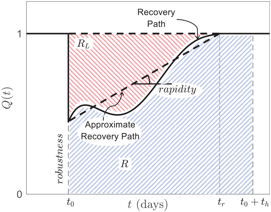
Schematic of a resilience triangle.

The value of $R_L$ is in the units of time. In terms of a desirable attribute, resilience $R$ is better defined as system functionality normalized with respect to uninterrupted functionality across the time horizon $t_h$ (also called control time of the system) (Bocchini and Frangopol, 2011; Cimellaro et al., 2010):

$$R=\frac{1}{t_h}{\int }_{t_0}^{t_0+t_h}Q(t)\mathrm{d}t.$$

(4)

The length of time horizon $t_h$ is based on the time span of interest. Longer values of $t_h$ are considered for community-based resilience, whereas smaller values are adopted for building-focused decisions.

In this article, the resilience metrics of three representative reinforced concrete (RC) moment frame buildings conforming to Canadian codes (CSA A23:3, 2014; NBCC, 2015) are assessed. The buildings are selected to represent the seismic behavior of a class of buildings (D’Ayala et al., 2014; FEMA P695, 2009). These buildings are designed and detailed for the seismicity of Vancouver, British Columbia. Housing occupancy has been considered as the performance metric for post-earthquake recovery of buildings. Effects of building heights on the resilience metrics are studied using 3-, 6-, and 9-story buildings. The nonlinear analytical models of buildings are subjected to two sets of ground motion records (FEMA P695, 2009), far-field (FF) and near-field (NF), to capture the effects of pulse and directivity in time history. The probabilistic framework for resilience assessment is applied by defining appropriate functional states (Burton et al., 2016). These functional states split the building recovery process into disjoint branches depending on the activities required to restore the building’s housing occupancy. Furthermore, a scenario earthquake of magnitude 7.3 in the Strait of Georgia at a distance of 30 km from the site is simulated to assess the recovery trajectory of buildings. Recovery trajectory of buildings in terms of housing occupancy as a function of time after the scenario earthquake is developed. Monte Carlo simulations are used to propagate the uncertainty in the resilience metric, starting with the seismic hazard to the building behavior to the lead time required for building recovery. Finally, the time required for buildings to achieve different recovery targets is assessed.

Adopted seismic resilience framework

Burton et al. (2016) extended the concepts of PBSD to assess seismic resilience considering the probabilistic performance of buildings. They considered housing occupancy, the capacity of buildings in terms of occupants, as a system performance metric. Housing occupancy for a building can broadly take one of the three functional states—no occupancy (NOcc), loss of occupancy (OccLoss), or full occupancy (OccFull). In the post-earthquake scenario, a building can follow different recovery paths to attain the same functional state. For example, a building remains unoccupiable while an inspection is due or if it is irreparably damaged and requires demolition and replacement. A set of disjoint event tree-based recovery paths is defined to incorporate the effects of externalities and socioeconomic factors in the recovery estimation. Figure 2 shows the adopted procedure for seismic resilience. An event tree approach with disjoint branches is considered. Depending on the extent of damage to the building and post-earthquake recovery activities, each branch is associated with a discrete damage state, $D{S}_i;i\in \{0,1,2,3,4,5\}$ . On two extremes, $D{S}_0$ indicates no damage to the building (operational), whereas $D{S}_5$ denotes collapse. Furthermore, Limit states, $L{S}_i;i\in \{1,2,3,4,5\}$ , are defined to demarcate among the different damage states. Following the PBSD framework, engineering demand parameters ( $\mathrm{EDP}$ ) are used to define thresholds for $L{S}_i$ . The probability of a building to achieve $D{S}_i$ after an earthquake event $I$ is expressed as

$$P[D{S}_i|I]=F[L{S}_i|I]-F[L{S}_{i+1}|I];i\in \{1,2,3,4\},$$

(5)

where $F[·]$ represents the cumulative density function and is obtained by fragility analysis. The tail probabilities are calculated trivially as $P[D{S}_0|I]=1-F[L{S}_1|I]$ and $P[D{S}_5|I]=F[L{S}_5|I]$ . Conditional housing capacity, $q(t)|D{S}_i$ , is assessed by breaking down different lead times needed for the post-earthquake activities to restore the building’s full occupancy.

Figure 2.

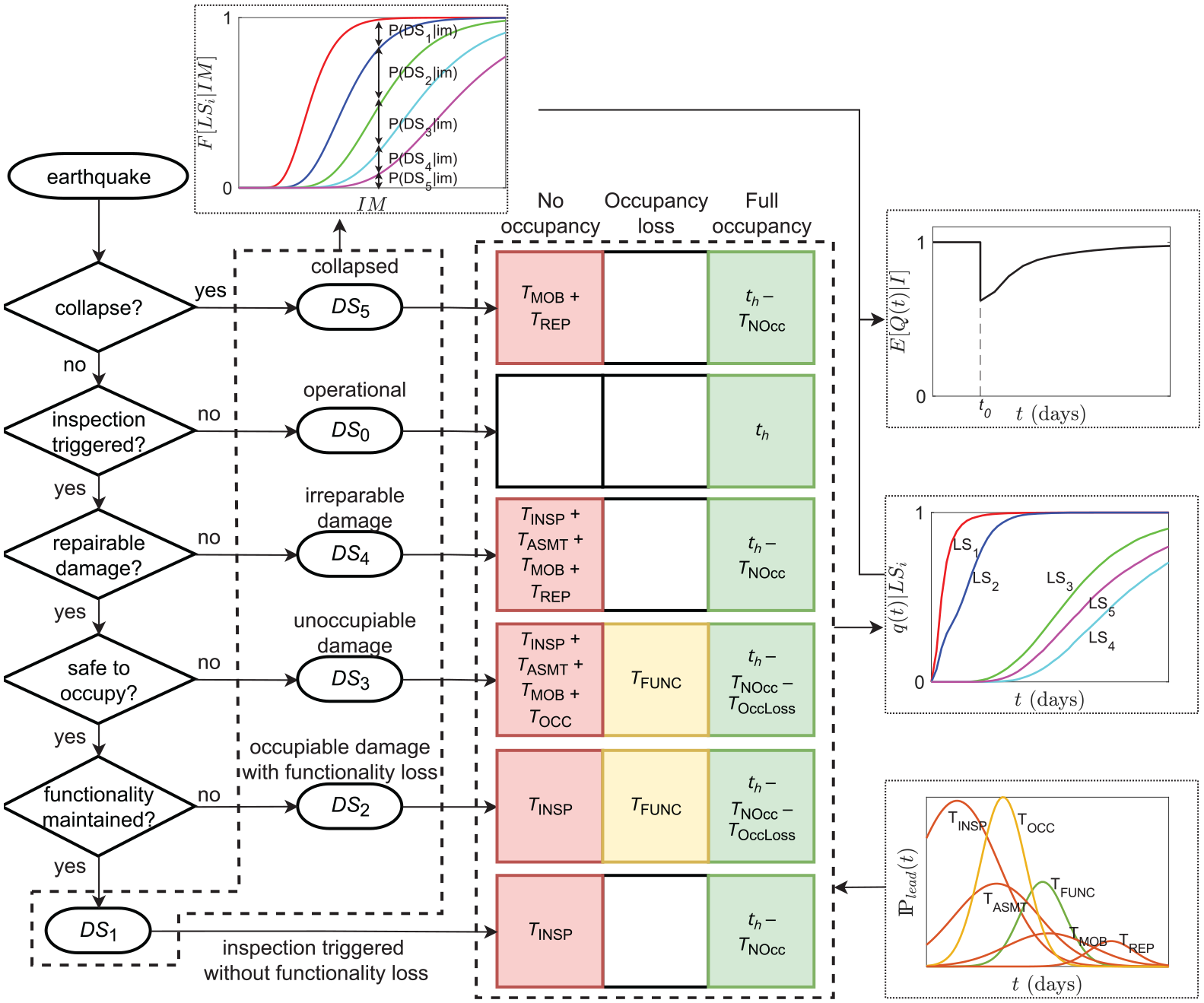
Procedure for probabilistic seismic resilience after an earthquake using an event tree approach.

Figure 2 shows a possible combination of necessary lead time components for each damage state. The time spent in NOcc and OccLoss are denoted by $T_{\mathrm{NOcc}}$ and $T_{\mathrm{OccLoss}}$ , respectively. After experiencing an earthquake, a building can achieve any of the six damage states from $D{S}_0$ to $D{S}_5$ with different probabilities as expressed by Equation 5. An inspection is triggered for all but two extreme damage states of $D{S}_0$ (operational) and $D{S}_5$ (collapse). The time variable for inspection is denoted by $T_{\mathrm{INSP}}$ . Time variable for functionality restoration, detailed assessment, mobilization of construction work, occupancy restoration, and building replacement are denoted by $T_{\mathrm{FUNC}}$ , $T_{\mathrm{ASMT}}$ , $T_{\mathrm{MOB}}$ , $T_{\mathrm{OCC}}$ , and $T_{\mathrm{REP}}$ , respectively. A high degree of uncertainty is associated with each activity. Several studies in the past (such as Almufti and Willford, 2013; Cook et al., 2022; FEMA P-58, 2012, etc.) have carried out realistic estimates of distribution of lead times and modeled them as lognormal random variables. The present study adopts this assumption from the literature. Fragility functions for each limit state is developed using incremental dynamic analysis (IDA) for a suitable ground motion set (Baker, 2015; Vamvatsikos and Cornell, 2002). If $q(t)|D{S}_i$ is housing occupancy conditional on damage state $D{S}_i$ , the total probability theorem can be used to determine the expected housing occupancy for that building as

$$E[Q(t)|I]=\sum _{i=0}^{n_{\mathrm{ls}}}[q(t)|D{S}_i]P[D{S}_i|I],$$

(6)

where $n_{\mathrm{ls}}$ is the number of the limit states and $E[·]$ is the expected value operator. While the impeding factors for building recovery can be captured following the REDi methodology (Almufti and Willford, 2013), the present study evaluates a benchmark resilience of typical code-conforming RC buildings in Canada, these factors are implicitly captured in the lead time variables and are not considered specific to each building. Effects of these externalities can be incorporated by modifying the lead times required for different recovery activities as discussed later. The equivalence between functionality loss and damage states is based on Burton et al. (2016). In the present study, damage state $D{S}_2$ corresponds to a maintained occupancy with functionality loss. For buildings in $D{S}_2$ , once the inspection is complete, functionality restoration activities can be directly initiated while the building remains partially occupied. The damage state $D{S}_1$ corresponds to the damage triggering inspection without loss of functionality. The damage state $D{S}_3$ is defined as unoccupiable building requiring evacuation until the restoration for occupancy is complete. When a building experiences $D{S}_3$ , inspection, detailed assessment, and mobilization of repair activities are undertaken. The building becomes partially occupied as soon as the occupancy restoration is complete and becomes fully occupied only after functionality recovery is complete. The damage state $D{S}_4$ corresponds to irreparable damage requiring the building to be replaced as soon as the inspection and assessment are complete. The damage state $D{S}_5$ corresponds to collapse. A building in $D{S}_5$ does not require an inspection and detailed assessment due to unambiguous collapse. A descriptive correspondence between functional damage states and performances is given by the Building Seismic Safety Council (BSSC, 2009) and described quantitatively in the section on Fragility in this article.

Example RC buildings conforming to Canadian standards

In the present study, three building configurations with 3, 6, and 9 stories have been selected to obtain a baseline resilience of typical code-conforming ductile RC moment-resisting frame (MRF) buildings in Canada (Noh and Tesfamariam, 2018). Selected buildings are assumed to be located at a hypothetical site in Vancouver City Centre with coordinates ${49}^{°}{15}^{\prime }{00}^{\prime \prime }\mathrm{N}$ , ${123}^{°}{6}^{\prime }{00}^{\prime \prime }\mathrm{W}$ . 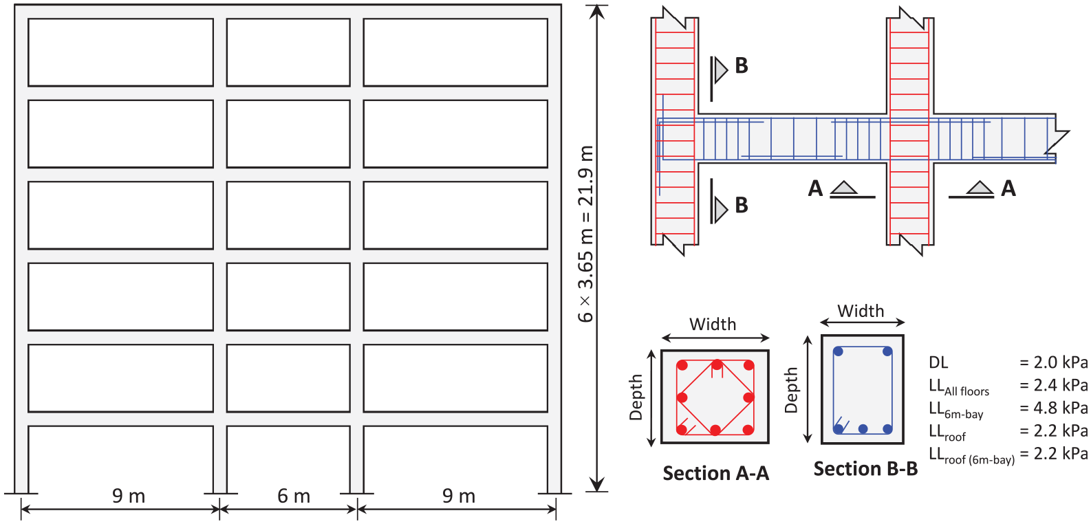Figure 3 shows the typical elevation of the buildings having three bays along the shorter direction. In the transverse direction, there are seven bays at 6 m spacing. Each story is 3.65 m in height. The selected buildings are founded on soft rock ( $V_{s30}=450\mathrm{m}/\mathrm{s}$ ). The seismic design of the buildings was carried out using the equivalent lateral force method as per NBCC (2015) and CSA A23:3 (2014).

Figure 3.

Details of the 6-story RC moment-resisting frame building under study (Noh and Tesfamariam, 2018).

The ductility and overstrength-related force modification factors are considered as $R_d=4.0$ and $R_o=1.7$ , respectively. Table 1 lists the basic design details of buildings. The approximate period $T_a$ specified by NBCC (2015) and design base shear coefficients for buildings are also given in Table 1. Design base shear value ranges from 3.6% to 7.8% of seismic weight. Concrete with compressive strength $f_c^{\prime }$ of 30 MPa and reinforcement steel of characteristic yield strength $f_y$ of 400 MPa were used as material for RC sections. More details on loads, design, and detailing for the buildings are provided in Table 1. The table also shows the maximum base shear capacity, $C_{s,\max }$ , based on nonlinear static analysis.

Table 1.

General building details for RC moment frame buildings

Number of stories	$T_a$ (s)	$T_1$ (s)	$C_{s,D}$ (%)	$C_{s,\max }$ (%)	$R_{o,p}$
3	0.45	0.83	7.8	29.5	3.8
6	0.76	1.68	4.5	12.4	2.7
9	1.03	2.41	3.6	8.4	2.3

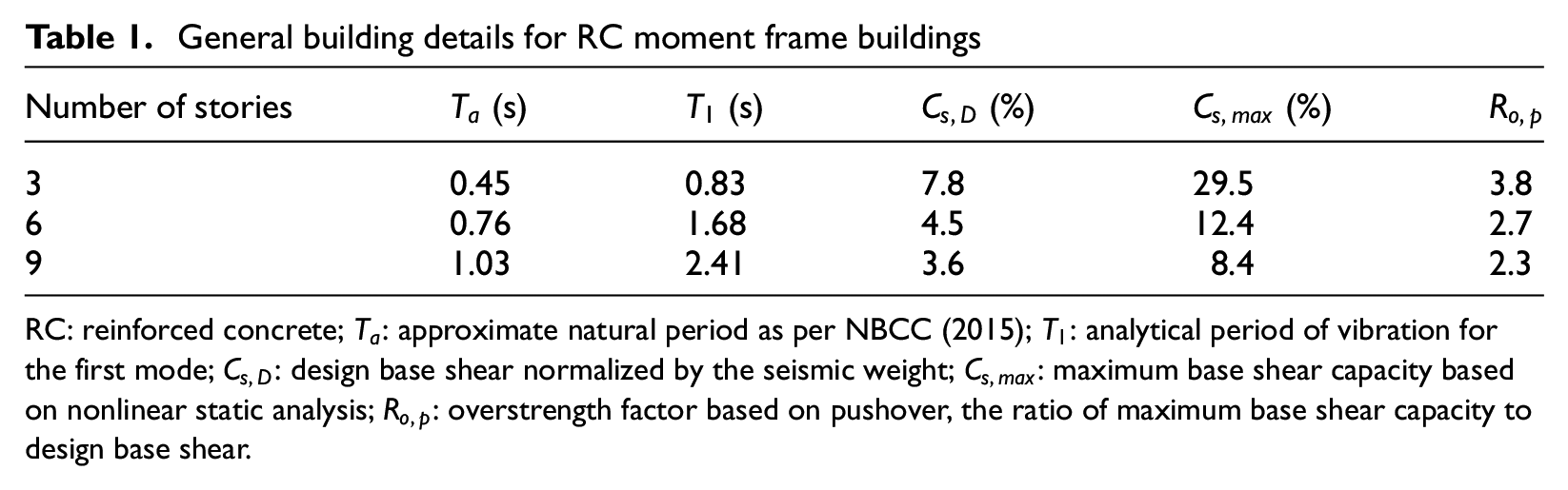
RC: reinforced concrete; $T_a$ : approximate natural period as per NBCC (2015); $T_1$ : analytical period of vibration for the first mode; $C_{s,D}$ : design base shear normalized by the seismic weight; $C_{s,\max }$ : maximum base shear capacity based on nonlinear static analysis; $R_{o,p}$ : overstrength factor based on pushover, the ratio of maximum base shear capacity to design base shear.

Nonlinear assessment model

A two-dimensional analytical model with concentrated plasticity is developed in OpenSees (McKenna et al., 2000) for numerical simulations. Due to the regularity of buildings, flexural hinges located on the beam–column joints have been considered to be sufficient for capturing nonlinear behavior. The effects of soil and foundation are accounted for using additional flexural hinges at the bottom. Their stiffness is approximated based on ASCE 41-17 (2017) for shallow foundations. Shear hinges are not modeled due to the capacity-based shear design of ductile RC columns per clause 21.3.2.7.1 of CSA A23:3 (2014). Several experimental (Ebrahimian et al., 2018; Jeong and Elnashai, 2004) and analytical studies (ATC 78-1, 2012; Badal and Sinha, 2022) support this modeling assumption by showing that the capacity-based shear design ensures a dominant flexural failure preceding the shear failure. The geometric nonlinearities (P-Δ effect) in columns are modeled using a leaning column that simulates additional gravity loads (Geschwindner, 2002). The backbone curve and hysteretic rules for frame members are defined following Ibarra–Medina–Krawinkler (IMK) model (Ibarra et al., 2005). The key parameters are determined using semi-empirical relations (Haselton et al., 2016; Panagiotakos and Fardis, 2001). These studies exploit a large available database of RC experiments (Berry et al., 2004). The yield moment and curvature are based on Panagiotakos and Fardis (2001), whereas the effective stiffness has been considered as secant stiffness to 40% of the yield value proposed by Haselton et al. (2016):

$$\frac{E{I}_{\mathrm{stf}40}}{E{I}_g}=-0.02+0.98\nu +0.09\frac{L_s}{H},\mathrm{where}0.35\le \frac{E{I}_{\mathrm{stf}40}}{E{I}_g}<0.80,$$

(7)

where $E{I}_{\mathrm{stf}40}$ is the secant stiffness to 40% yield moment, $E{I}_g$ is the gross stiffness, $\nu =P/f_c^{\prime }{A}_g$ is the axial load ratio for expected gravity loads, and $L_s/H$ is the ratio of shear span to the depth of the member. The capping moment capacity, $M_c$ is given as

$$\frac{M_c}{M_y}=1.25(0.89{)}^{\nu }(0.91{)}^{0.01f_c^{\prime }}.$$

(8)

Similarly, the plastic rotation component to the capping rotation ${\theta }_{\mathrm{cap},\mathrm{pl}}$ and the post-capping rotation ${\theta }_{\mathrm{pc}}$ are based on the axial load ratio and the volumetric transverse steel ratio, ${\rho }_{\mathrm{sh}}$ . The effect of bond-slip is captured in the estimation of plastic rotation capacity. Figure 4 shows the schematic diagram of a sub-assemblage of the analytical model. The finite size of the beam–column joint has been modeled using the compression strut mechanism (Lowes and Altoontash, 2003). Table 2 gives modeling details of members of example buildings on the ground floor. Rayleigh damping of 5% is employed in the first and the third modes. The damping is considered only in the pre-yielding members to avoid the numerical pitfalls that may result in excessive fictitious energy dissipation (Hall, 2006; Petrini et al., 2008). The maximum base shear capacity based on pushover analysis is shown in Table 1. The overstrength factor, $R_{o,p}$ , of the example buildings, defined as the ratio of maximum base shear capacity from pushover analysis to the design base shear, is found to be between 2.3 and 3.8, which is typical of modern lateral load-resisting frames (ASCE 7, 2016; NBCC, 2015).

Figure 4.

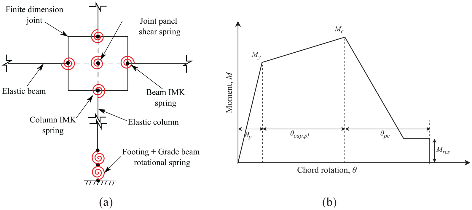
Schematic details of the nonlinear analytical model for ductile RC frames: (a) the sub-assemblage (Badal and Sinha, 2022) and (b) a typical backbone curve (Ibarra et al., 2005).

Table 2.

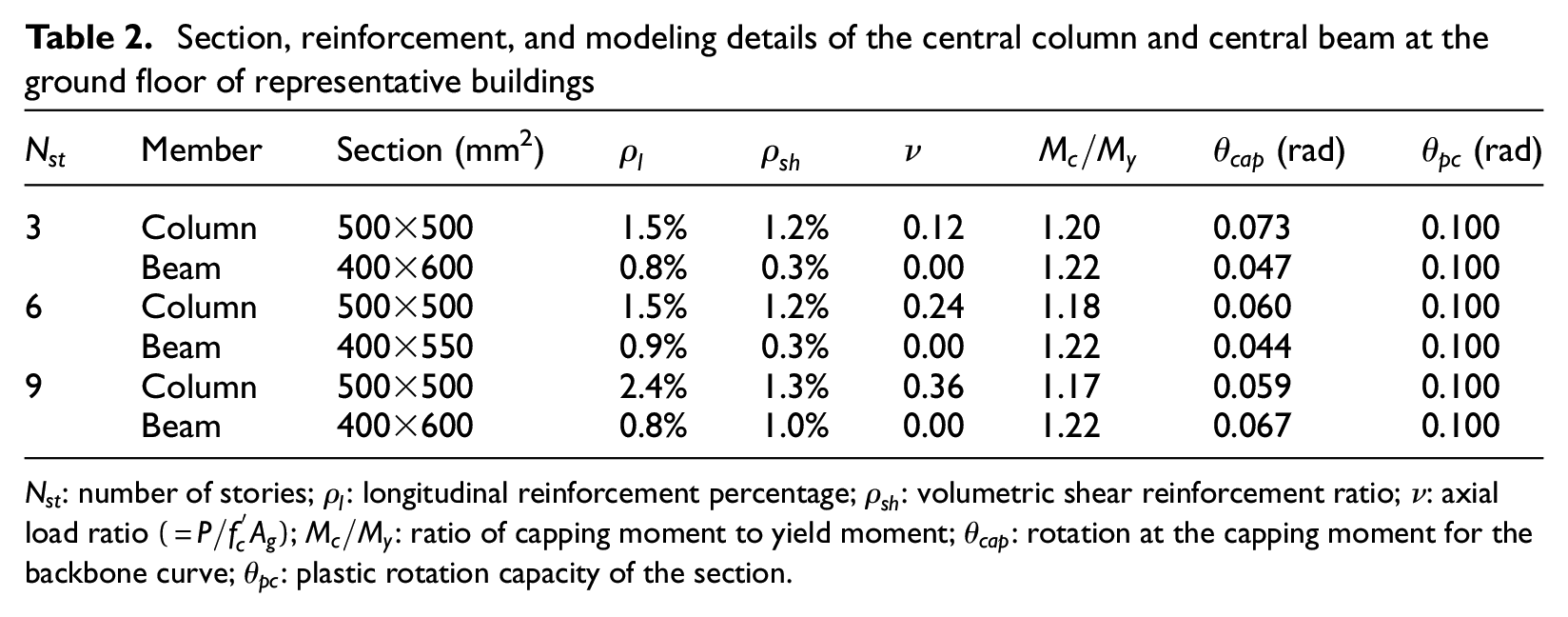
Section, reinforcement, and modeling details of the central column and central beam at the ground floor of representative buildings

$N_{\mathrm{st}}$	Member	Section (mm2)	${\rho }_l$	${\rho }_{\mathrm{sh}}$	$\nu$	$M_c/M_y$	${\theta }_{\mathrm{cap}}$ (rad)	${\theta }_{\mathrm{pc}}$ (rad)
3	Column	$500\times 500$	1.5%	1.2%	0.12	1.20	0.073	0.100
	Beam	$400\times 600$	0.8%	0.3%	0.00	1.22	0.047	0.100
6	Column	$500\times 500$	1.5%	1.2%	0.24	1.18	0.060	0.100
	Beam	$400\times 550$	0.9%	0.3%	0.00	1.22	0.044	0.100
9	Column	$500\times 500$	2.4%	1.3%	0.36	1.17	0.059	0.100
	Beam	$400\times 600$	0.8%	1.0%	0.00	1.22	0.067	0.100

$N_{\mathrm{st}}$ : number of stories; ${\rho }_l$ : longitudinal reinforcement percentage; ${\rho }_{\mathrm{sh}}$ : volumetric shear reinforcement ratio; $\nu$ : axial load ratio $(=P/f_c^{\prime }{A}_g)$ ; $M_c/M_y$ : ratio of capping moment to yield moment; ${\theta }_{\mathrm{cap}}$ : rotation at the capping moment for the backbone curve; ${\theta }_{\mathrm{pc}}$ : plastic rotation capacity of the section.

Fragility analysis

For a given building, fragility function $F_{L{S}_i}(\mathrm{im})$ gives its probability of exceeding the limit state $L{S}_i$ as a function of the intensity measure $\mathrm{IM}$ . Depending on the objective and rigor of the study, various methods are adopted to assess the fragility function (Baker, 2015). The present study has adopted an IDA approach (Vamvatsikos and Cornell, 2002). Under IDA, each record in a selected ground motion set is increasingly scaled until the building collapses or reaches extreme deformation levels. Seismic fragility is frequently expressed as a lognormal distribution. Intensity measure values required to exceed a limit state for each ground motion record in a suite are combined statistically to ascertain the median and record-to-record uncertainty of the fragility function. In addition to record-to-record variation, ${\beta }_{\mathrm{RTR}}$ , unaccounted sources of uncertainty are approximated using FEMA P-695 guidelines as follows: (1) uncertainty in modeling, ${\beta }_{\mathrm{MDL}}=0.35$ : Fair rating with medium confidence in RC special moment frame models, (2) uncertainty in test data, ${\beta }_{\mathrm{TD}}=0.20$ : Good rating due to well-calibrated RC beam–column data, and (3) uncertainty in design requirements, ${\beta }_{\mathrm{DR}}=0.10$ : Superior rating on account of capacity-based RC frame design. Four components are combined using the square root of the sum of their squares to obtain the total uncertainty, ${\beta }_{\mathrm{TOT}}$ . Two ground motion sets of FEMA P695 (2009) are considered for analyses. Based on the minimal difference in the predicted median capacity of 1-, 4-, and 12-story RC special moment frame buildings in Appendix A of FEMA P695 (2009), these sets are considered to be broadly applicable for the benchmark study of all buildings (3–9 stories tall) in the present study. The distance to the source was used to develop separate FF and NF ground motion sets. The high-velocity pulse anticipated in the NF sites is captured sufficiently using NF sets for various structures (Dimakopoulou et al., 2013; Jäger and Adam, 2013).

Figure 5a shows hazard curves for spectral acceleration at natural period of each building based on draft NBCC (2020) seismic hazard maps (Kolaj et al., 2020) for Vancouver ( ${49}^{°}{15}^{\prime }{00}^{\prime \prime }\mathrm{N}$ , ${123}^{°}{6}^{\prime }{00}^{\prime \prime }\mathrm{W}$ ) on a site with the average shear-wave velocity in the top 30 m of soil, $V_{s30}=450\mathrm{m}/\mathrm{s}$ . Figure 5b and c shows 22 pairs of FF and 28 pairs of NF ground motion records. The scaled response spectrum of Vancouver is also shown in the figure to compare the spectral shape of these records. The site hazard is scaled such that its $\mathrm{Sa}(T=1\mathrm{s})$ matches the median of $\mathrm{Sa}(T=1\mathrm{s})$ for each suite. This scaling is only carried out for the comparison of spectral shapes. A wide range of spectral ordinates in the elastic response spectrum indicate the inherent variability in the ground motion. A close match of Vancouver’s response spectrum with the median of FF records is also noted. The NF set exhibits a large uncertainty in the short period range, reflecting pulse effects in the time-history records.

Figure 5.

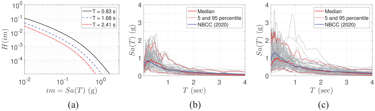
(a) Seismic hazard of Vancouver site as per proposed seismic maps of NBCC (2020), (b) 22 pairs of far-field, and (c) 28 pairs of near-field ground motion records (FEMA P695, 2009). Solid blue lines represent Vancouver’s response spectrum per NBCC (2020). To compare the spectral shape of records, the site’s $\mathrm{Sa}(T=1\mathrm{s})$ is scaled to match with the median of $\mathrm{Sa}(T=1\mathrm{s})$ for both suites.

Figure 6 shows IDA curves for 3-story buildings for both ground motion sets. A larger dispersion in the building capacity for a higher drift ratio is noted in the case of the NF records than in the FF records. The $\mathrm{Sa}(T_1)$ ( $T_1$ given in Table 1), is considered as $\mathrm{IM}$ . Furthermore, the geometric mean of spectral acceleration along two orthogonal directions is equally scaled for IDA (Whittaker et al., 2011). This scaling method is also consistent with the ground motion models, which usually estimate the geometric mean of spectral ordinates (Baker and Cornell, 2006). Finally, due to the use of two-dimensional models, the controlling component from each orthogonal pair of time–history records is used for the fragility.

Figure 6.

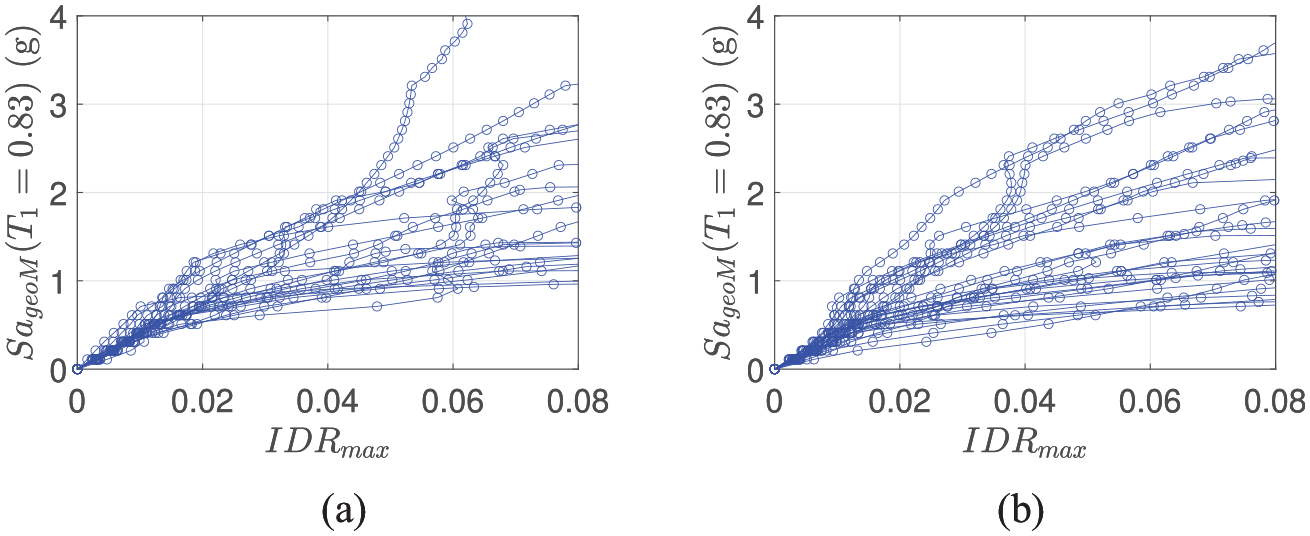
IDA curves of 3-story building for controlling components of (a) far-field and (b) near-field ground motion records. $\mathrm{ID}{R}_{\max }$ represents the maximum interstory drift ratio.

Figure 7 shows the fragility of all buildings using FF and NF records with ${\beta }_{\mathrm{RTR}}$ . In the present context of resilience assessment, limit state $L{S}_2$ is defined at the yield displacement of the idealized pushover curve. The limit state $L{S}_1$ is adopted as midway to $L{S}_2$ . The limit state $L{S}_3$ is defined when the rotation at any column hinge exceeds 50% of capping rotation capacity, given that the no floor has interstory drift of more than 2%. This limit ensures story-level damage, while the former captures element-level damages. The limit state $L{S}_4$ is defined when rotation at any column hinge exceeds the capping rotation capacity or the interstory drift on any floor exceeds 4%. The limit state $L{S}_5$ of collapse is established using IDA when the building experiences exorbitant story drifts or a sidesway instability due to story mechanism. These definitions are based on extensively studies in the literature (D’Ayala et al., 2014; Dolšek and Fajfar, 2008; Yepes-Estrada et al., 2016).

Figure 7.

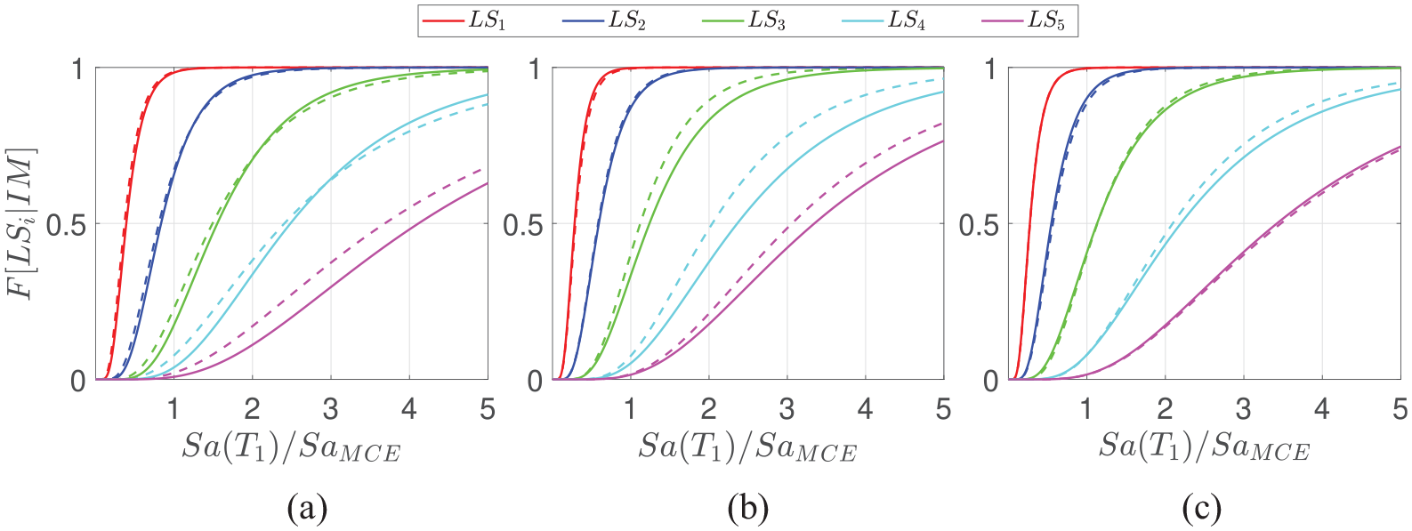
Fragility functions for (a) 3-story, (b) 6-story, and (c) 9-story buildings for far-field (FF) and near-field (NF) ground motion suites. Solid and dashed lines correspond to the fragility function using FF and NF ground motions, respectively. The fragility functions are plotted only with ${\beta }_{\mathrm{RTR}}$ components.

The median and record-to-record uncertainty parameters for the fragility functions are listed in Table 3. Median capacity ${\mu }_{L{S}_i}$ is normalized by the maximum considered earthquake (MCE) level design spectral acceleration, $\mathrm{Sa}(T_1{)}_{\mathrm{MCE}}$ , for the site. It is noted from the table that on an average, the MCE-level event (i.e. ${\mu }_{L{S}_i}/\mathrm{Sa}(T_1{)}_{\mathrm{MCE}}=1$ ) results all buildings to exceed limit state $L{S}_2$ . It is also noted that for 3- and 6-story buildings, the median collapse capacity ( ${\mu }_{L{S}_5}$ ) is smaller using the NF ground motion records compared with FF ground motion records. On the contrary, the fragility of the 9-story building for all limit states remains largely unchanged for both NF and FF ground motion records. For example, the 3-story building has a ${\mu }_{L{S}_5}/\mathrm{Sa}(T_1{)}_{\mathrm{MCE}}$ value of 4.11 for the FF ground motion set, which reduces to 3.68 for NF records. Furthermore, the probability of exceeding the irreparable damage state conditional on MCE ground motion $F_{L{S}_4}(\mathrm{MCE})$ is calculated to be 3.9% for FF ground motion and 7.7% for NF ground motion records. This indicates that the seismic capacity of low- and mid-rise buildings is significantly affected by ground motion records’ pulse and directivity effects.

Table 3.

Fragility function parameters for RC moment frame buildings for different limit states

$N_{\mathrm{st}}$	GM	$T_1$	${\mu }_{L{S}_i}/\mathrm{Sa}(T_1{)}_{\mathrm{MCE}}$					${\beta }_{\mathrm{RTR},L{S}_i}$
	Suite	(s)	$L{S}_1$	$L{S}_2$	$L{S}_3$	$L{S}_4$	$L{S}_5$	$L{S}_1$	$L{S}_2$	$L{S}_3$	$L{S}_4$	$L{S}_5$
3	FF	0.83	0.33	0.71	1.55	2.48	4.11	0.15	0.16	0.22	0.30	0.42
	NF	0.83	0.31	0.67	1.49	2.40	3.68	0.18	0.22	0.34	0.45	0.49
6	FF	1.68	0.28	0.60	1.24	2.36	3.34	0.13	0.18	0.28	0.33	0.37
	NF	1.68	0.28	0.59	1.12	2.04	3.06	0.14	0.17	0.20	0.27	0.33
9	FF	2.41	0.27	0.61	1.13	2.20	3.43	0.14	0.20	0.31	0.37	0.39
	NF	2.41	0.26	0.59	1.14	2.10	3.48	0.17	0.20	0.26	0.32	0.40

RC: reinforced concrete; FF: far-field; NF: near-field; GM: ground motion.

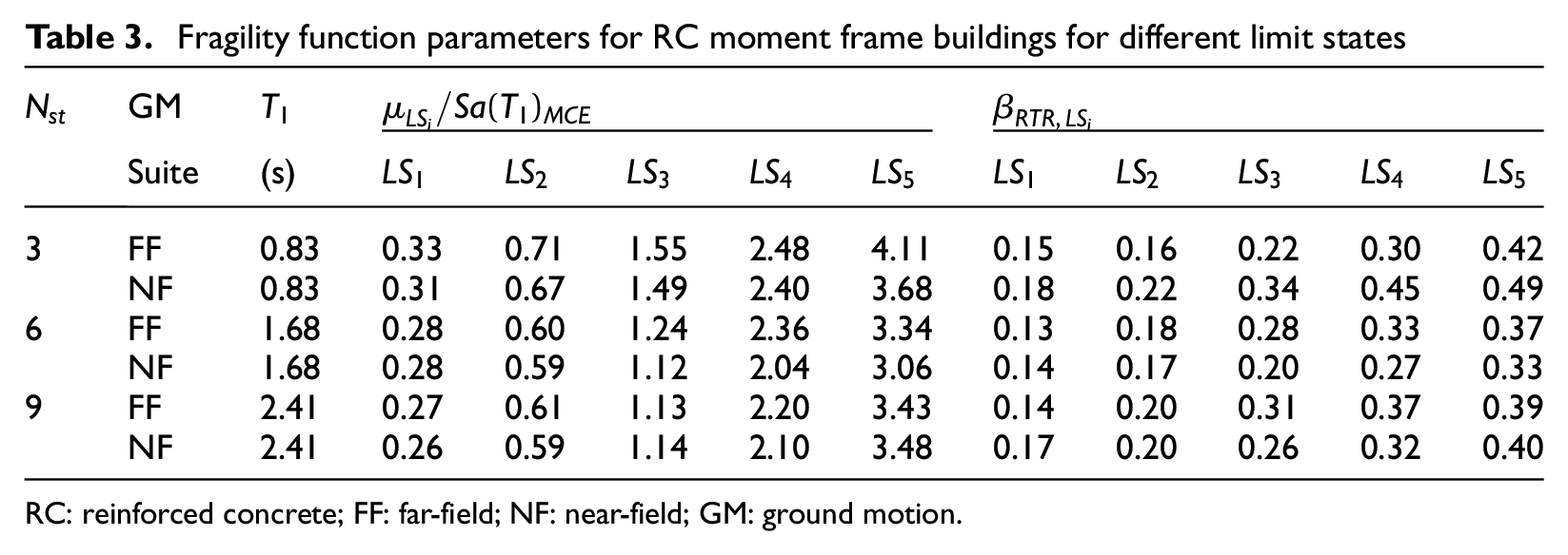
Seismic damages to nonstructural components of a building can lead to significant economic losses and downtime (Liel and Deierlein, 2013; Porter et al., 2001). Observations from past earthquakes substantiate these findings (Ding et al., 1990; McKevitt et al., 1995). A nonstructural component is typically classified as either drift-sensitive (interstory drift ratio, $\mathrm{IDR}$ ) or acceleration-sensitive (peak floor acceleration, $\mathrm{PFA}$ ). In the present study, the fragility for nonstructural components are developed based on the median $\mathrm{EDP}$ demand for different components as given by fragility database of FEMA P-58-3 (2018). As an example, Figure 8 shows the IDA curves for acceleration-sensitive components and the fragility for suspended ceilings (component ID C3032.001a) for 3-story building for FF ground motion records. Table 4 shows the median EDP demand and median capacity for different nonstructural components of all buildings corresponding to FF ground motion set. The nonstructural component were selected based on the normative quantity estimation tool (FEMA P-58-3, 2018) and local construction practices for buildings in Canada. At the end, the structural median capacity of buildings ascertained earlier is shown for comparison with nonstructural components. It is noted that for these buildings, nonstructural components are typically damaged at higher intensity measure values than the structural damage itself. Similar results (not shown here for brevity) are obtained for NF ground motion set.

Figure 8.

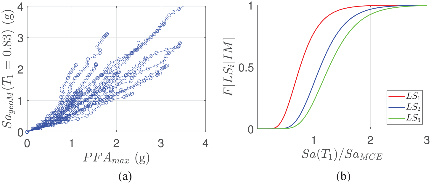
For the 3-story building, (a) IDA curves for peak floor acceleration PFA and (b) fragility functions using FF ground motions for suspended ceilings.

Table 4.

Fragility function parameters for nonstructural components of RC moment frame buildings for different limit states corresponding to far-field ground motion set

Component	$\mathrm{EDP}$	Median demand a			${\mu }_{L{S}_i}/\mathrm{Sa}(T_1{)}_{\mathrm{MCE}}$
		$L{S}_1$	$L{S}_2$	$L{S}_3$	3-story			6-story			9-story
					$L{S}_1$	$L{S}_2$	$L{S}_3$	$L{S}_1$	$L{S}_2$	$L{S}_3$	$L{S}_1$	$L{S}_2$	$L{S}_3$
Wall partition b	IDR (%)	0.5	1.0	2.1	0.39	0.84	1.61	0.28	0.59	1.30	0.27	0.55	1.19
Suspended ceiling c	PFA (g)	1.17	1.58	1.82	1.73	2.56	2.92	1.54	2.09	2.38	1.47	1.93	2.18
Potable piping d	PFA (g)	1.5	2.6	–	2.41	3.75	–	1.99	3.17	–	1.85	2.86	–
HVAC e	PFA (g)	1.5	2.25	–	2.41	3.42	–	1.99	2.85	–	1.85	2.56	–
Sprinkler piping f	PFA (g)	1.1	2.4	–	1.58	3.59	–	1.44	2.99	–	1.39	2.69	–
Sanitary piping g	PFA (g)	1.2	2.4	–	1.79	3.59	–	1.59	2.99	–	1.51	2.69	–
Structural	–	–	–	–	0.33	0.71	1.55	0.28	0.60	1.24	0.27	0.61	1.13

RC: reinforced concrete; IDA: interstory drift ratio; PFA: peak floor acceleration.

a

Based on FEMA P-58-3 (2018).

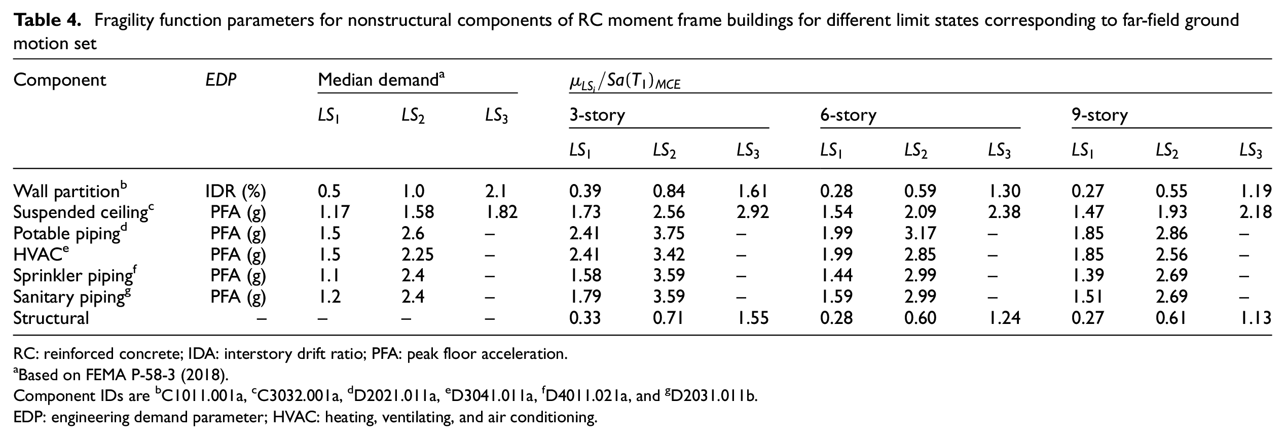
Component IDs are ^bC1011.001a, ^cC3032.001a, ^dD2021.011a, ^eD3041.011a, ^fD4011.021a, and ^gD2031.011b.EDP: engineering demand parameter; HVAC: heating, ventilating, and air conditioning.

Housing occupancy

Normalized housing occupancy is taken as the system performance metric in the present study. It is defined as the ratio of absolute housing occupancy to pre-earthquake housing capacity. In the probabilistic framework, recovery curves of buildings provide the mean system performance as a function of the time after the earthquake. Table 5 shows the lead time distribution for different recovery activities of the 6-story building based on Burton et al. (2016). The lead time for each activity is modeled as a lognormal random variable with parameters as given in Table 5. The times required for mitigation activities are estimated based on the sequence of repairs. The statistical distributions of lead times consider structural as well as nonstructural damages. This captures the effects of losses to nonstructural members. For example, the lead time required for mobilizing, $T_{\mathrm{MOB}}$ , accounts for the related nonstructural damages. Similarly, the time spent to maintain functionality, $T_{\mathrm{FUNC}}$ , includes the repair time for building contents, planning of repair, and so on. Thus, the parameters of both $T_{\mathrm{MOB}}$ and $T_{\mathrm{FUNC}}$ are dependent on the nonstructural damages. The logarithmic uncertainty ${\sigma }_{\ln }$ of 0.40 is considered in the lead times for functionality restoration, occupancy restoration, and replacement. Higher uncertainty in inspection, assessment, and mobilization is expected due to the increased demand in the aftermath of the earthquake. This is captured by assigning ${\sigma }_{\ln }$ of 0.75. The values of dispersion are based on FEMA P-58 (2012). The ${\sigma }_{\ln }$ values of 0.40 and 0.75 result in ≈ 84% observations (within 1 standard deviation) to be less than 1.5 and 2.0 times the median lead time, respectively. The replacement time for 3- and 9-story buildings are considered 210 and 400 days, respectively. The lead times required for preliminary inspection ( $T_{\mathrm{INSP}}$ ), engineering assessment ( $T_{\mathrm{ASMT}}$ ), and mobilization for construction ( $T_{\mathrm{MOB}}$ ) do not typically vary for low- and mid-rise buildings. Similarly, the activities for functionality and occupancy restoration allow access to different parts of buildings (event tree in Figure 2), and parallel repair activities can be undertaken for low- to mid-rise buildings. Thus, the associated lead times, $T_{\mathrm{OCC}}$ and $T_{\mathrm{FUNC}}$ , are considered to have the same distribution. It is worth noting that these lead times are a crude estimation of recovery activities and socioeconomic factors, including the location of the building. Such factors can be adjusted by amplifying the lead times based on real-life evidence.

Table 5.

Lead time distribution used for assessment of repair time for the 6-story RC building

Damage state	Median lead time
	$T_{\mathrm{INSP}}$ a	$T_{\mathrm{FUNC}}$ b	$T_{\mathrm{ASMT}}$ a	$T_{\mathrm{MOB}}$ a	$T_{\mathrm{OCC}}$ b	$T_{\mathrm{REP}}$ b
$D{S}_1$	30	–	–	–	–	–
$D{S}_2$	30	90	–	–	–	–
$D{S}_3$	30	120	60	150	45	–
$D{S}_4$	30	–	60	240	–	300
$D{S}_5$	–	–	–	240	–	300

RC: reinforced concrete.

a

${\sigma }_{\ln }=0.75$

b

${\sigma }_{\ln }=0.40$ .

Mean repair time

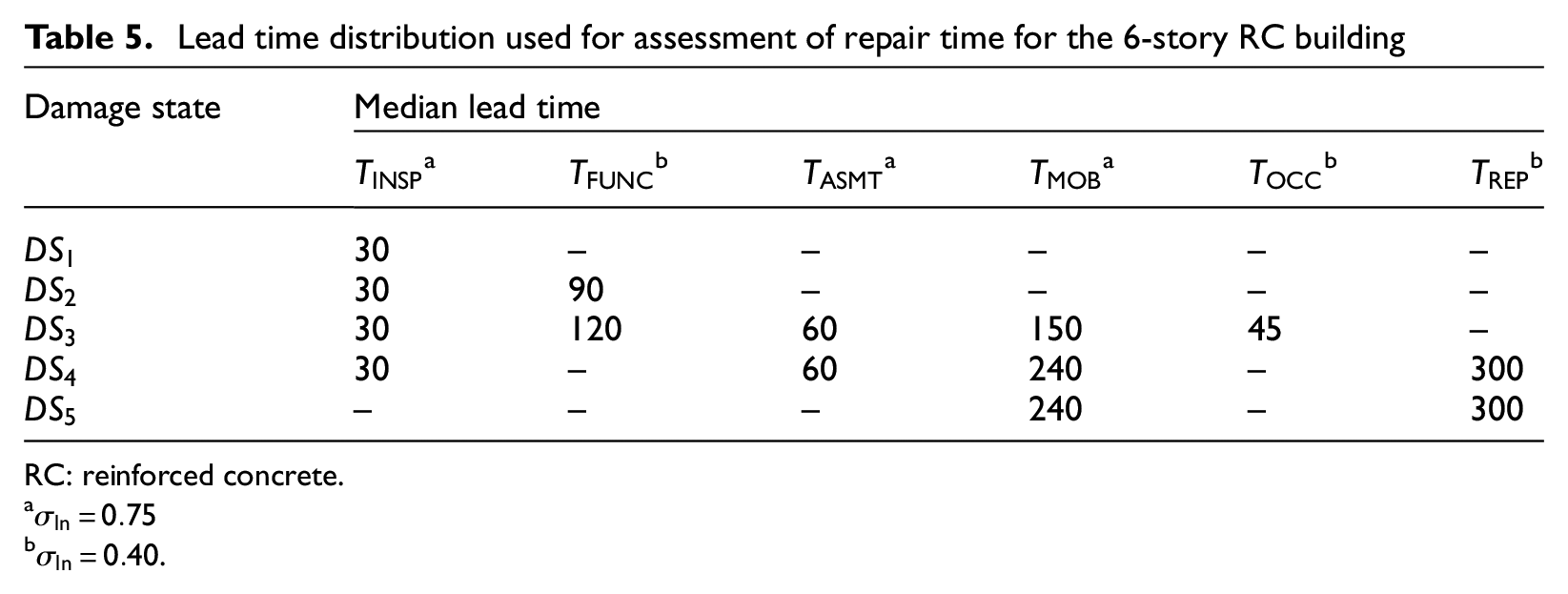
The mean repair time is the time required for the building to become fully occupiable after the inspection, assessment, and mobilization for the construction are complete. In practice, the time required before mobilization can be extraneously long (or, short) on account of safety cordons from nearby buildings, prioritization, or other owner-specific reasons. Hence, we present the mean repair time as a useful measure of the recovery process in the present section. For the normalized housing occupancy (in the following section), this effect is captured through a higher uncertainty associated with the distribution of $T_{\mathrm{INSP}}$ , $T_{\mathrm{ASMT}}$ , and $T_{\mathrm{MOB}}$ . Figure 11a shows the mean repair time as a function of intensity measure for all buildings under the study. The path to recovery is based on the event tree shown earlier in Figure 2. The mean repair time is calculated by combining the randomized realizations of lead times as follows:

$$\mathrm{Mean}\mathrm{repair}\mathrm{time}(\mathrm{im})=\sum _{i=1}^{n_{\mathrm{ls}}}P[D{S}_i|\mathrm{im}][T_{\mathrm{FUNC}\cup \mathrm{OCC}\cup \mathrm{REP}}|D{S}_i],$$

(9)

where $P[D{S}_i|\mathrm{im}]$ is defined earlier in Equation 5, and $T_{\mathrm{FUNC}\cup \mathrm{OCC}\cup \mathrm{REP}}|D{S}_i$ is the combined lead time required for occupancy, functionality restoration, and replacement conditional on the building exceeding damage state $D{S}_i$ . Monte Carlo simulations are used for the calculation of repair time. The intensity measure is normalized by the MCE-level spectral acceleration corresponding to 2% in 50-year probability. Different sources of uncertainty are considered in the assessment of repair time (and subsequently, resilience) by using the total uncertainty, ${\beta }_{\mathrm{TOT}},$ in the building fragility. The estimation of ${\beta }_{\mathrm{TOT}}$ values has been described previously. It is observed that an MCE-level intensity measure results in approximately 80–140 days of mean repair time for the example buildings. It is observed that the mean repair time does not exhibit a noticeable difference in FF and NF ground motion records for 3- and 9-story buildings. While this is attributed to the counteracting effects of a reduction in the median capacity and increase in dispersion for 3-story buildings (Table 3), the fragility parameters of the 9-story building are similar for both ground motion suites. Furthermore, uncertainty in the repair time is shown in Figure 11b. The process is noted to be heteroscedastic (changing variance with the intensity measure). The standard deviation varies between 0.4 and 0.2 with higher uncertainties for smaller intensity measures where damages are subjected to functionality restoration and occupancy restoration.

Housing occupancy for damaged buildings

Figure 9 shows the conditional housing occupancy $q(t)|D{S}_i$ for buildings subjected to different states after an earthquake. The probabilistic distribution of $q(t)|D{S}_i$ is determined using various lead time components for each damage state, as shown in Figure 2. Lead time components are assumed to be uncorrelated for simplicity. The figure shows clear segregation of the distributions for damages more severe than $D{S}_2$ . This is attributed to the time-consuming additional recovery activities, such as assessment, mobilization, occupancy restoration, and possibly, replacement of the building, required for these damage states. It is also observed from the figure that a building in damage state $D{S}_4$ takes longer than buildings in $D{S}_5$ . This is attributed to the additional time required for inspection and assessment of irreparably damaged buildings ( $D{S}_4$ ) than the unambiguously collapsed buildings ( $D{S}_5$ ).

Figure 9.

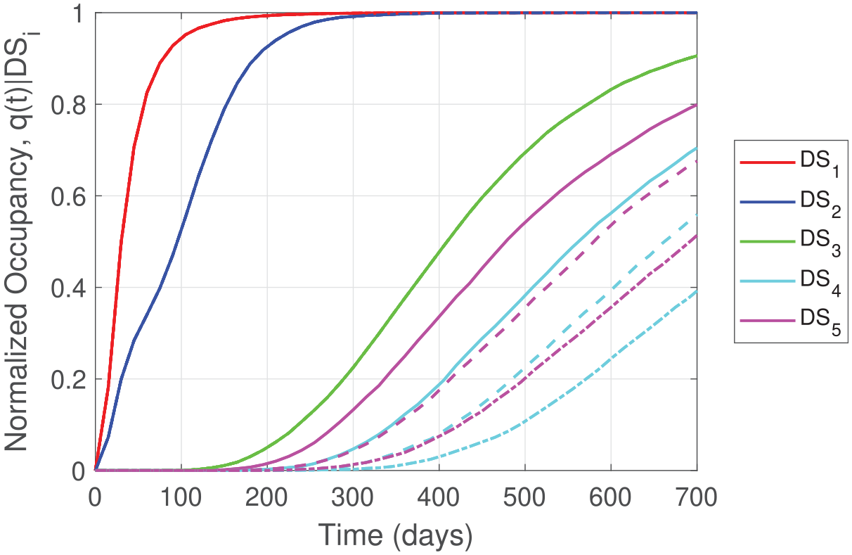
Distribution of normalized housing occupancy for different damage state as a function of time for 3-, 6-, and 9-story buildings. For damage states $D{S}_1$ , $D{S}_2$ , and $D{S}_3$ , all three buildings have the same conditional distribution of lead time. Solid and dashed lines correspond to the mean and uncertainty assessed using FF and NF ground motions, respectively.

Resilience of RC moment frame buildings for a scenario earthquake

Based on the historical seismicity of Vancouver, a 7.3 magnitude earthquake in the Strait of Georgia was characterized by Cassidy et al. (2000). This scenario was also considered by the City of Vancouver (2013) for earthquake preparedness and by Costa et al. (2022) for estimating population displacement. Thus, in the present section, resilience metrics of example RC frame buildings are assessed for the scenario earthquake of $M=7.3$ and a Joyner–Boore distance (the closest distance to the surface projection of an extended fault) of $R_{\mathrm{JB}}=30$ km.

Housing recovery trajectory

The scenario earthquake was simulated using the ground motion model proposed by Boore et al. (2014) for shallow crustal earthquakes. This ground motion model has also been used in the latest seismic hazard model of Canada (Kolaj et al., 2020). For a fixed magnitude–distance tuple, the uncertainty in the system performance metric propagates from the hazard (intensity measure distribution; captured using ground motion models) to the building fragility to the lead times for various recovery activities. In the present study, Monte Carlo simulations with 10,000 realizations are used to propagate the uncertainty. The total aleatory uncertainty function, representing the combination of between-event variability and within-event variability, is used for the simulations. For each realization, the housing occupancy following an earthquake is estimated using the building’s structural damage states (with different probabilities of being in damage states $D{S}_0$ through $D{S}_5$ ) and corresponding lead times for each event branch of the recovery tree. Depending on the accrued damage, a building will remain in one or more of the three functional states (Nocc, OccLoss, OccFull) for different durations. The housing occupancy in OccLoss, when the functionality restoration is ongoing, is assumed to be 40% of the pre-earthquake occupancy. Furthermore, using Equation 6 and the fragility functions (with ${\beta }_{\mathrm{TOT}}$ ) developed earlier, the expected recovery trajectory is calculated as a function of time $t$ .

Figure 10a shows the recovery trajectory for each building for normalized housing occupancy after the scenario earthquake. The figure shows the trajectory using both ground motion sets. The effect of two ground motion sets on the recovery path is minuscule. This is contrasted against the significantly different conditional probabilities of irreparable damage in the case of MCE-level events. It is observed from the figure that 9-story building experiences higher post-earthquake damages (less robust) and has a longer recovery period (reduced rapidity). It is anticipated that the 9-story building also has a higher loss of resilience over the time horizon. Furthermore, Figure 10b shows the uncertainty in the recovery trajectory. The standard deviation varies between 0.10 and 0.35 with higher uncertainties in the aftermath of the earthquake. The uncertainty reduces with the reduction in the burden of restoration activities.

Figure 10.

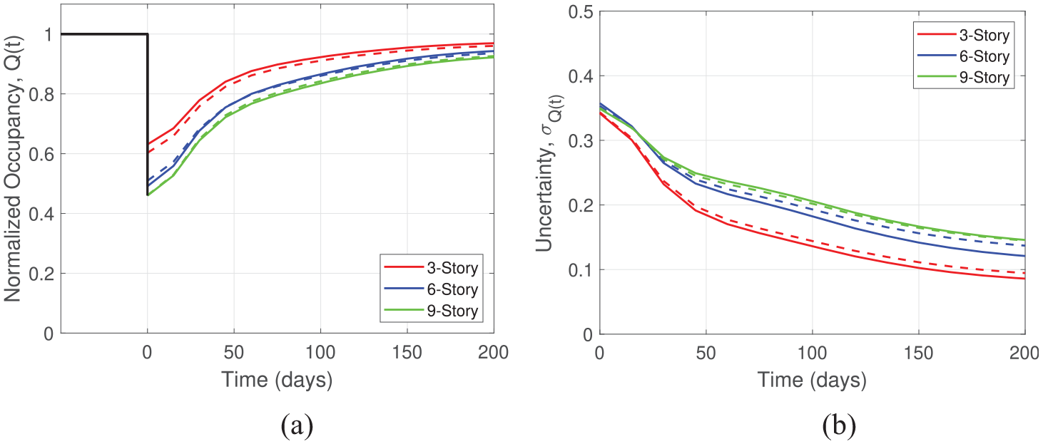
Housing recovery functions for Vancouver for a scenario earthquake of magnitude, $M=7.3$ , and distance, $R_{\mathrm{JB}}=30$ km, for 3-, 6-, and 9-story RC frame buildings. Solid and dashed lines correspond to the recovery function using FF and NF ground motions, respectively. (a) Mean and (b) uncertainty in the housing recovery function.

Resilience metrics and recovery targets

Table 6 shows three resilience metrics for example buildings. The 3-story building is more robust than the 6- and 9-story buildings. In the aftermath of the scenario earthquake, the housing occupancy of the 3-story example building is reduced by an average of 35%, whereas the housing occupancy of 6- and 9-story buildings is reduced by ~ 50%. The shape of the recovery path is closer to exponential as the relative rapidity reduces with time. This validates the assumptions made in other studies (e.g. Tirca et al., 2016). The rapidity is noted to be higher for taller buildings. This is attributed to the high levels of damage experienced by these buildings and hence, increased levels of recovery activities. The total resilience of buildings with housing occupancy as the system performance metric is shown in the last three columns of the table. The time horizon $t_h$ is decided with the building-related decisions in the short-term. Thus, $t_h$ is adopted equal to the duration after which resilience is estimated for each column. After 1 month of the event, approximately half of the 6- and 9-story buildings’ resilience is lost ( $R=$ 54%–58%). Three-story buildings experience a loss of approximately one-third of their resilience in this duration ( $R=$ 67%–69%). For a target resilience of 90%, the 3-story building requires approximately 6 months, whereas taller buildings take almost a year to achieve that level of resilience.

Table 6.

Robustness, rapidity, and resilience for the housing capacity in case of a scenario earthquake of magnitude, $M=7.3$ and distance, $R_{\mathrm{JB}}=30$ km

$N_{\mathrm{st}}$	GM	Robustness	Rapidity $(\mathrm{yea}{\mathrm{r}}^{-1})$			Resilience
	Suite		30 days	180 days	365 days	30 days	180 days	365 days
3	FF	65%	1.80	0.68	0.35	69%	88%	93%
	NF	62%	1.90	0.72	0.37	67%	86%	92%
6	FF	49%	2.26	0.90	0.48	57%	81%	88%
	NF	51%	2.11	0.85	0.45	58%	81%	88%
9	FF	46%	2.25	0.92	0.49	54%	78%	86%
	NF	46%	2.29	0.93	0.50	54%	78%	86%

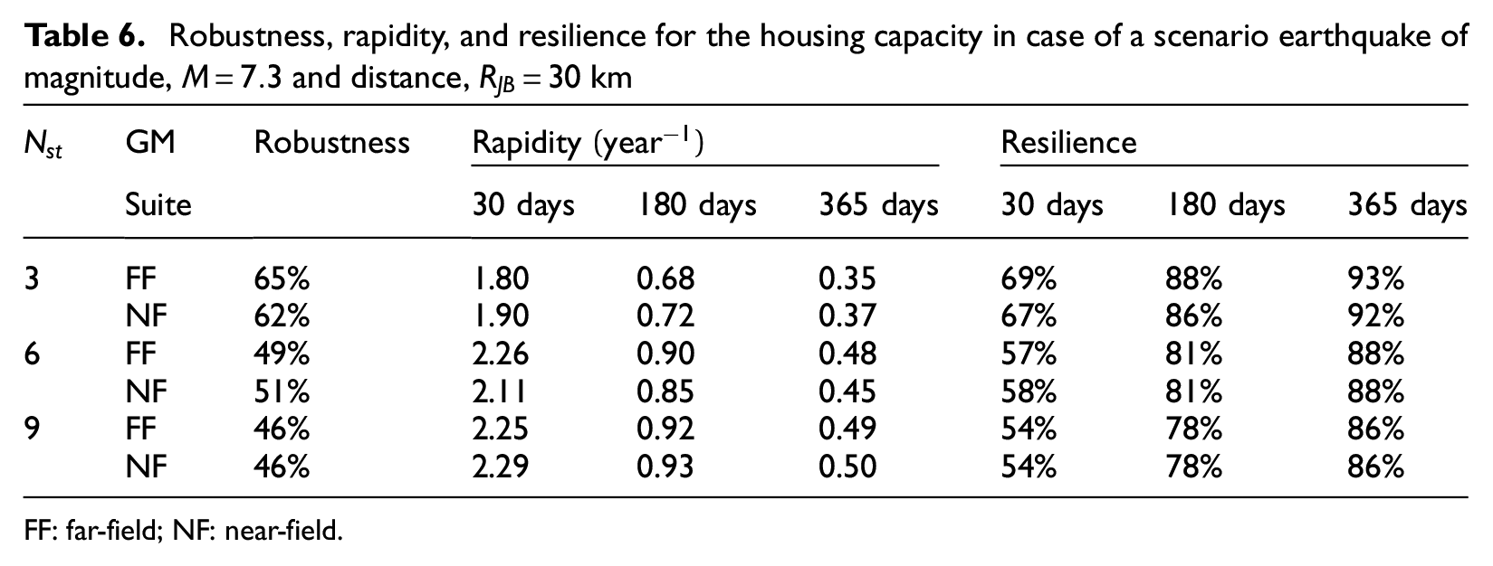
FF: far-field; NF: near-field.

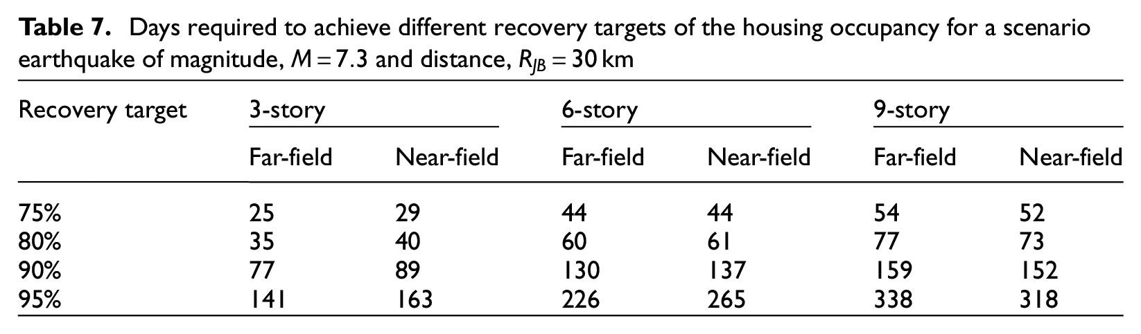
The recovery of a system represents its performance at a specified point in time, whereas its resilience represents the accumulated loss of performance over the time horizon. Table 7 shows the number of days required to meet different recovery targets. It is noted that for the scenario earthquake of 7.3 magnitude at a distance of 30 km, 90% of recovery in the housing capacity is attained within 3–5 months by all buildings. However, as noted earlier, it takes much longer (6 months to 1 year) for the building to achieve similar levels of resiliency.

Table 7.

Days required to achieve different recovery targets of the housing occupancy for a scenario earthquake of magnitude, $M=7.3$ and distance, $R_{\mathrm{JB}}=30\mathrm{km}$

Recovery target	3-story		6-story		9-story
	Far-field	Near-field	Far-field	Near-field	Far-field	Near-field
75%	25	29	44	44	54	52
80%	35	40	60	61	77	73
90%	77	89	130	137	159	152
95%	141	163	226	265	338	318

Comparison with field observations

In this section, we compare the analytically obtained repair time with the empirical field observations. Although the database used for the comparison is taken from American buildings, they provide insight into the estimated and observed repair times. For two major earthquakes on the North American pacific coast, 6.9 magnitude Loma Prieta (1989) and 6.7 magnitude Northridge (1994), extensive reconnaissance studies have been undertaken to assess economic losses and building damages (Eguchi et al., 1998; Kroll et al., 1991). However, limited empirical data on the recovery time and functionality restoration exist in the literature. Comerio and Blecher (2010) examined 4937 buildings tagged with red and yellow after the two earthquakes for their repair and re-occupancy time. The mean time to occupancy for multi-family buildings (considered suitable for comparison with 3- to 9-story buildings considered in the present study) after the Loma Prieta (1989) earthquake in Hollister, at $R_{\mathrm{JB}}=28\mathrm{km}$ from the epicenter, was reported as 14 months. For a Hollister—South & Pine site (RSN-776 in the PEER database) on the stiff rock, the ratio $\mathrm{Sa}(T_1)/S{a}_{\mathrm{MCE}}$ for 3-, 6-, and 9-story buildings (T₁ = 0.83, 1.68, and 2.41 s) is calculated as 1.15, 1.21, and 1.08, respectively (Ancheta et al., 2014). Due to a combination of the distance (i.e. $R_{\mathrm{JB}}\ge 20\mathrm{km}$ ) and the lack of pulse in time history, the comparison is made with FF ground motion set. From the present study, Figure 11a and b shows the mean repair time as a function of $\mathrm{Sa}(T_1)/S{a}_{\mathrm{MCE}}$ . For the FF ground motion suite, the predicted mean repair times are 185, 249, and 304 days (i.e. 6–10 months) for 3-, 6-, and 9-story buildings, respectively. This estimate is on the lower side than the empirically observed 14 months. Similarly, the mean time to occupancy after the Northridge (1994) earthquake in unincorporated Los Angeles county, at a distance of 32 km from the epicenter, was reported as 13 months. For the nearby site Sylmar—Converter Station East (RSN-1085 in the PEER database) on stiff rock, the ratio $\mathrm{Sa}(T_1)/S{a}_{\mathrm{MCE}}$ for 3-, 6-, and 9-story buildings (T₁ = 0.83, 1.68, and 2.41 s) is calculated as 2.34, 2.44, and 2.25, respectively (Ancheta et al., 2014). Using Figure 11a and b, the mean repair times are predicted as 100, 146, and 155 days (i.e. 3–5 months). This estimate is also on the lower side than the empirically observed 13 months for Northridge for sites near the recording station. The differences are attributed to the inferior quality of buildings at that time. Furthermore, the mixed building types, including premodern lateral load-resisting systems, are expected to sustain higher damages leading to longer repair time.

Figure 11.

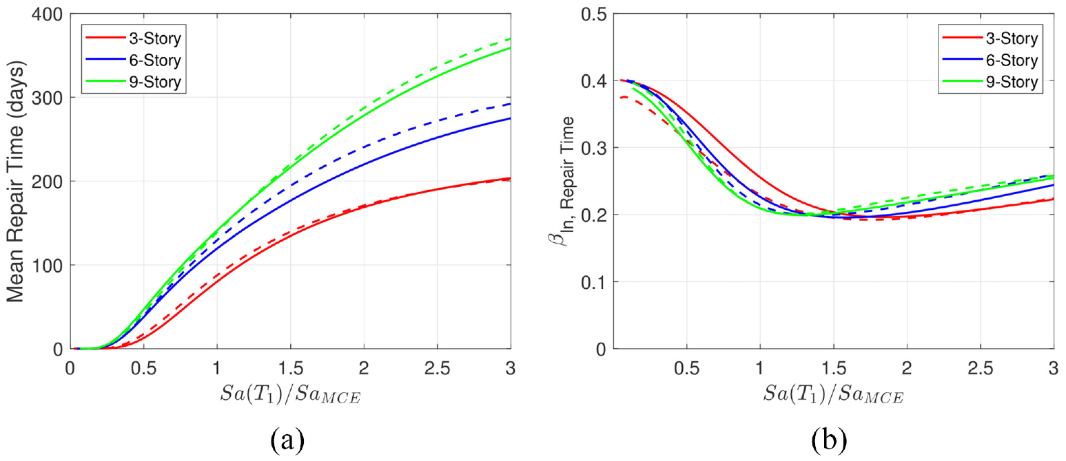
(a) Mean repair time as a function of normalized intensity measure for each building assessed for FF (far-field) and NF (near-field) ground motion suite, (b) logarithmic uncertainty in the repair time. Solid and dashed lines correspond to the mean and uncertainty assessed using FF and NF ground motions, respectively.

Summary and conclusion

Seismic design standards and the research community are gradually moving toward a performance-based design. Such methodology allows the design of buildings to meet specified levels of decision variables such as collapse, injury, dollar loss, or casualty. However, the variation of system performance (such as occupancy or functionality loss) over time in the aftermath of an event remains unknown. Various stakeholder groups like governments, housing communities, and owners can benefit from the information on the recovery and resilience of buildings to choose suitable design goals.

The present study evaluated the seismic resilience of ductile RC moment frame buildings conforming to Canadian seismic design and detailing standards (CSA A23:3, 2014; NBCC, 2015). Different resilience metrics for robustness, rapidity, and resilience are examined against a disruptive event. These metrics capture system’s reliability, speed of recovery, and socioeconomic impacts, respectively. Three representative buildings of 3-, 6-, and 9-stories in height are selected to assess the baseline resilience of code-conforming RC moment frames. Housing occupancy as a fraction of pre-earthquake occupancy has been considered as the system performance metric. Nonlinear time-history analyses are performed by subjecting buildings to two ground motion sets. Due to proximity to the active faults, NF effects are captured using the NF ground motion set. Damage states are defined for each event branch depending on the need for different activities such as inspection, detailed assessment, mobilization for construction, occupancy restoration, functionality restoration, and replacement. The distributions of normalized housing occupancy for each damage state as a time function are developed.

An earthquake of magnitude 7.3 in the Strait of Georgia at a distance of 30 km from the site is simulated to assess the recovery trajectory of buildings. The study uses the event tree approach to present the mean recovery path of the normalized housing occupancy following the simulated earthquake event. Large levels of uncertainty in the resilience metric exist even for a fixed magnitude–distance tuple. This uncertainty has been propagated from the hazard to the building fragility to the lead times for various recovery activities using Monte Carlo simulations. The resulting mean recovery path of each building represents the probabilistic trajectory of the housing occupancy in the scenario earthquake. Finally, the time required to achieve different recovery targets is estimated.

The following main conclusions are drawn from the study:

1. The mean repair time required to complete inspection, assessment, and mobilization for construction, for a 3-story RC moment frame building is lower than that for 6- and 9-story buildings. However, for an MCE-level event, the mean repair time of 3–4 months is comparable for all three buildings.

2. The effect of NF ground motion is pronounced in the low-rise buildings compared with taller buildings. The probability of irreparable damage conditional on an MCE-level event for the 3-story building is 3.9% for the FF ground motion set, whereas it increases to 7.7% for the NF ground motion set.

3. The normalized housing occupancy for different damage states as a function of time is developed for all buildings. These results, along with a suitable ground motion model, can be used to obtain a recovery trajectory for any scenario earthquake.

4. In the aftermath of a scenario earthquake of 7.3 magnitude at 30 km distance from the example site, the 3-story building is found to be ~ 65% robust, whereas taller buildings are ~ 50% robust.

5. For the scenario earthquake, 90% of housing recovery is attained within 3–5 months by all buildings, with taller buildings recovering slower than shorter ones. However, it takes much longer (6 months to a year) for system resilience to achieve similar levels across the time horizon.

6. Field observations from two similar earthquakes on the North American pacific coast, Loma Prieta (1989) and Northridge (1994), indicate that the recovery time for the special RC moment frame considered in the present study is lower than empirically observed data from these well-recorded past earthquakes.

Socioeconomic factors, including the location of the building, can affect different lead times significantly. In the aftermath of an earthquake, an imbalance in demand-supply for construction-related activities can decelerate the recovery. On the contrary, government intervention can alleviate some of the burdens. Appropriate adjustments for such factors can be made by amplifying or reducing the lead times based on real-life evidence. The present study made several assumptions to obtain a benchmark resilience of representative ductile RC moment frame buildings conforming to Canadian codes. Resilience assessment can be further improved by accurate assessment of the damage states and lead time distributions. At the same time, due to the large inherent uncertainty in the ground motion, building behavior, and repair activities, while releasing these assumptions will result in a fine-grained resilience estimate, it is not anticipated to deviate largely from the current estimate. In addition, the validity of assumptions is tested by comparing the obtained mean repair time estimates from field observations.

Findings from the present study can be extended to estimate the demand for temporary shelters and disaster relief activities. The derived housing recovery function can further be integrated to estimate the overall loss in terms of person-days. Following the approach in the present study, robustness and resilience targets can be specified for the design of the new buildings or rehabilitation of the old ones. As also proposed in the literature (Ademovic and Ibrahimbegovic, 2020; Cimellaro, 2013; Fung et al., 2022), this shift from performance-based design to resilience-based design rooted in social metrics like occupancy, downtime, and so on, will equip decision-makers and communities to understand their risk better and eventually become more resilient.