Sage Journals: Discover world-class research

Abstract

The performance-based earthquake engineering (PBEE) methodology allows designers to deaggregate expected seismic losses in a building to a component level. This deaggregated information provides the opportunity to tailor upgrade strategies to individual structures based on sources of losses. However, the optimization of an upgrade strategy becomes difficult because of the relationship between a structure and its nonstructural components; hence, multiple competing upgrade options must be considered. To address this obstacle, this article proposes a framework to guide the assessment of the viability of both structural and nonstructural upgrade strategies, while accounting for limited design resources likely encountered in the early stages of the design process. The framework utilizes the median shift probability (MSP) method, a modified version of the PBEE method introduced in this article, to rapidly summarize the effects of structural upgrades on nonstructural components by considering the impacts of structural modifications on the floor hazards. While accounting for this relationship, the MSP method utilizes the deaggregation of loss across different source categories to identify the benefit of combined structural and nonstructural upgrades, increasing a designer’s understanding of the impact of structural upgrades on losses and allowing for the rapid determination of optimized upgrade strategies unique to the owner’s conditions. A case study example of the implementation of the framework is provided, and the results obtained from the MSP method are compared with those obtained from more rigorous but resource-intensive optimization analysis. An implementation of the MSP method in Microsoft Excel is provided with this article.

Keywords

Performance-based earthquake engineering holistic seismic design cost-benefit analysis rapid design optimization structural and nonstructural upgrades

Introduction

The development of the performance-based earthquake engineering (PBEE) methodology by the Pacific Earthquake Engineering Research (PEER) Center (Miranda and Aslani, 2003) has provided a process for quantifying earthquake-induced losses using performance measures that can be understood by a wide range of stakeholders. This methodology has highlighted the importance of considering both structural and nonstructural seismic losses in seismic design and retrofit (Bradley et al., 2009; Miranda and Taghavi, 2003). In parallel with general loss reduction considerations, seismic design guidelines such as American Society of Civil Engineers (ASCE) 41 (ASCE, 2017) and the resilience-based earthquake design initiative (REDi) rating system (Almufti and Willford, 2013) have been developed based on seismic performance targets, ranging from collapse prevention to immediate occupancy, and are applied to both structures and nonstructural components. However, while the performance of the structure and the nonstructural components is often treated independently in these design guidelines, the PBEE methodology captures the relationships between them (Bradley et al., 2009; Günay and Mosalam, 2013; O’Reilly and Calvi, 2020; Perrone et al., 2019). These relationships must be considered when evaluating seismic upgrades to a building, as the effect of these relationships can include: a reduction of expected benefits from the implementation of higher performing seismic force-resisting systems (SFRSs) if seismic upgrades to the nonstructural components are not considered; the benefits provided by upgrading the nonstructural components not being wholly achieved if the structure is not similarly robust; and changes in the dynamic properties of a structure due to structural upgrades impacting the engineering demand parameters (EDPs) imposed on the nonstructural components. Current PBEE evaluation methodologies capture these relationships implicitly through scenario-based evaluations, but do not encourage the implementation of an integrated and optimized upgrade strategy because they require a trial-and-error approach aided only by guidance from experienced designers.

A further challenge facing decision makers when attempting to reduce exposure to seismic loss is optimizing the upgrade investment. Recently, several studies have presented methods for comparing the costs and benefits of structural upgrades and have shown that implementing a high-performing SFRS can provide a net positive benefit. Galanis et al. (2018) used the PBEE methodology to evaluate the cost-benefit of structural seismic upgrades and demonstrated its use on two case-study residential buildings in Europe. Hofer et al. (2018) applied the PBEE methodology to determine a profitability index associated with various seismic retrofit strategies for an industrial facility. Recent researches by Cardone et al. (2019), Bianchi et al. (2021), and Arifin et al. (2021) have considered the impact of both structural and non-structural upgrades on the overall life-cycle cost of buildings. Most studies that use life cycle assessment to determine the viability of a seismic upgrade use as their metric either a net present value (NPV) or a benefit-cost ratio (BCR) calculation:

NPV = (EA L_{O} - EA L_{U}) AM - UC

(1)

BCR = \frac{EA L_{O} - EA L_{U}}{UC} AM

(2)

where EAL_O is the expected annual loss of the original (non-upgraded) building, EAL_U is the expected annual loss of the upgraded building, UC is the upgrade cost, and AM is an amortization conversion expressed by:

AM = (1 - \frac{1}{{(1 + r)}^{t}}) r^{- 1}

(3)

where r is the internal rate of return or discount rate, and t is the expected occupancy time of the building in years. Both the NPV and BCR equations compare the reduction in loss and the upgrade cost, where a positive value of NPV or a BCR value exceeding unity indicates that the proposed upgrade strategy yields a reduction in seismic losses that exceeds the implementation cost and is, therefore, viable. However, the studies described above limit the scope of the upgrade strategy to structural modifications, neglecting the effect of upgrading the nonstructural components.

In the study by Steneker et al. (2020), a methodology was developed to systematically determine optimal upgrade strategies when considering both structural and nonstructural components. For this purpose, a genetic algorithm (GA) was used to define each “individual” in a potential upgrade generation as a string of bits. Both structural and nonstructural upgrades were considered in each individual, and each change of a bit from a value of 0 to 1 corresponded to a component being seismically upgraded, resulting in a change to both the capital cost and estimated building loss. The flexibility of the algorithm allowed multiple target metrics, such as minimizing economic costs or downtime, including both upgrade costs and reduction in seismic losses. While a GA provides a systematic way of determining optimal seismic upgrades and significantly reduces the computational effort when compared to a brute force approach, its implementation can still be onerous during the preliminary phases of an upgrade feasibility study, where the full scope of the possible upgrade strategies is not yet defined. Furthermore, previous work has mostly measured the gains obtained from various upgrade strategies by comparing the reduction in the final loss value obtained from the PBEE methodology, using either a scenario- or time-based assessment (FEMA, 2018). This comparison of final values only indicates overall viability of the proposed upgrade strategy and does not provide detailed reasoning on the design and selection of the combination of structural and nonstructural upgrades. Such guidance would be valuable at the preliminary stages of decision-making.

To address these needs, this article presents a framework to guide decision-making when contemplating seismic upgrades. The goal is to provide a more formalized and accessible evaluation framework for practicing engineers and stakeholders who use PBEE to evaluate the viability of an upgrade through increasing layers of analytical complexity. The article first introduces a three-level framework for assessing the viability of seismic upgrades. The first two levels of this framework utilize a novel and rapid modification to the PBEE evaluation process, referred to as the median shift probability (MSP) method. The MSP is introduced in this article along with a summary of the required PBEE equations. The third level of this framework is implemented using the GA optimization presented in the study by Steneker et al. (2020). Finally, a case study is presented to illustrate the application of the framework and MSP method by initially assessing the viability of several potential structural upgrade strategies, before comparing the results of this assessment with the results obtained from the more rigorous Level 3 optimization process utilizing the GA.

Overview of proposed framework

The proposed framework divides the upgrade design and viability assessment into three distinct levels, as shown in Figure 1, where each level has increasing analytical refinement. Information on the original conditions of the structure, such as probability distributions describing the collapse, residual and floor hazard curves, are required to serve as a point of comparison. In Level 1, the cost of a proposed structural upgrade is estimated, and the associated changes to each of these curves that would be required to produce a positive NPV are obtained. These required changes are then assessed by the designer based on engineering judgment to determine whether they are likely to be achievable based on the proposed upgrade type. If so, the investment of the engineering resources required for a Level 2 analysis is justified, and a design of each upgrade and the development of corresponding analytical models is used to refine each upgrade curve. The results of this structural analysis are then used to confirm the positive NPV result for the structural upgrade before deciding whether to invest the additional resources required to fully optimize the upgrade strategy in Level 3.

Figure 1.

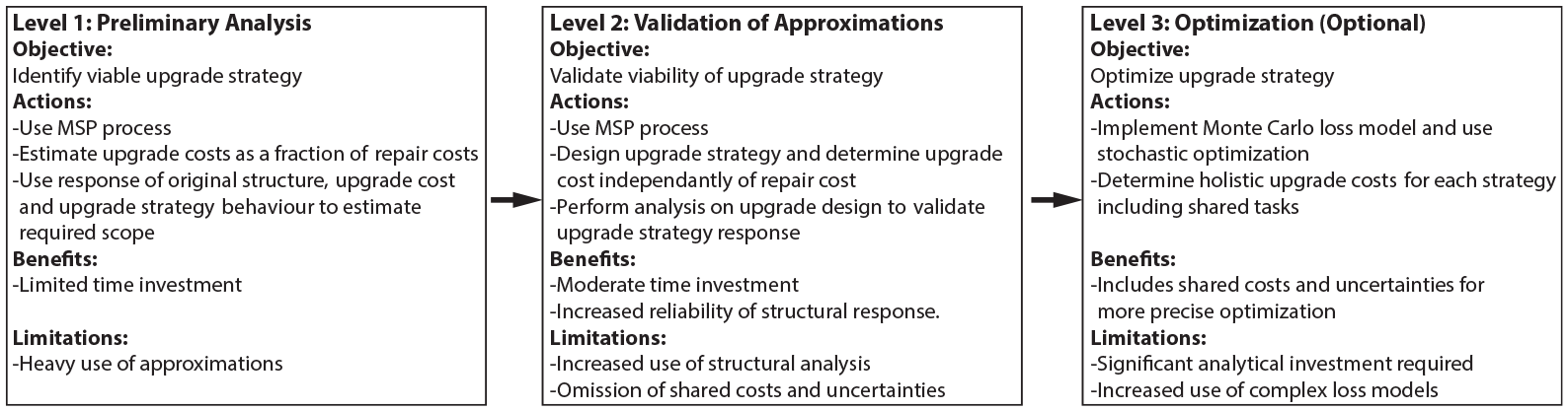
Levels of assessment of proposed framework to determine upgrade viability and optimization.

A modified PBEE method, the MSP method, is used for Levels 1 and 2 as it summarizes the change in structural performance by defining explicitly the relationship between changes to a structure and the resulting demands on nonstructural components. This provides an alternative to either the end-to-end total probability theorem (Günay and Mosalam, 2013) or Monte Carlo PBEE approaches (FEMA, 2018). The MSP method allows the viability of different upgrade strategies to be approximately quantified early in the decision-making process based on changes to single parameters of the probabilistic functions that describe key performance indicators. In particular, the relationship between changes to the behavior of the structure and the performance of the nonstructural components, defined as changes to the floor hazard curves, are expressed using these shifts in probabilistic functions. The importance of this relationship is further demonstrated by deaggregating the total change in loss with a particular upgrade strategy into distinct source categories.

Key parameters of MSP method

Performance of structures and nonstructural components

The seismic performance of structural systems or non-structural components is often quantified using a fragility curve that is represented by a lognormal cumulative distribution function (CDF):

p (D S_{k} | x) = Φ (\frac{\ln (\frac{x}{θ_{k}})}{β_{k}})

(4)

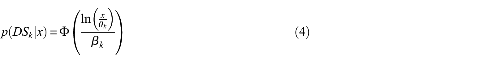
where p(DS_k|x) is the probability of occurrence of a specific damage state (DS) k (DS_k) given a hazard intensity x (e.g. ground spectral acceleration at first-mode period, peak floor acceleration), Φ is the standard Gaussian CDF, θ_k is the median intensity of x, and β_k is the standard deviation of the lognormal CDF. The probability of occurrence of events was used instead of the probability of exceedance to avoid the required subtraction of values when using probability of exceedance when determining specific event occurrence (FEMA, 2018). For structures, collapse fragility curves are used to define the probability of occurrence of structural collapse given a site hazard intensity measure (IM), typically represented by the spectral acceleration at the first-mode period (FEMA, 2009). This can be done based on incremental dynamic analysis or more computationally efficient alternatives, such as multiple stripe analysis (Baker, 2015), which generates the same two parameters that define the lognormal CDF (θ_k, β_k) using the maximum-likelihood estimation (MLE) method (Baker, 2015). For nonstructural components, similar lognormal CDFs are used to define the probability of occurrence of specific DSs given an EDP, instead of an IM. An extensive library of these curves for nonstructural components is included in the performance assessment calculation tool (PACT), developed as part of the FEMA P-58 project (FEMA, 2018). While some nonstructural components may be exposed to multiple simultaneous DSs (e.g. both guide rails and operational machinery being damaged for elevators), each with an independent probability of occurrence, the structural system and most nonstructural components have sequential and exclusive DSs (e.g. increasing quantities of plastic deformations in a connection) whose definition requires conditional probabilities. Capturing this exclusivity using the lognormal CDF functions is expressed as:

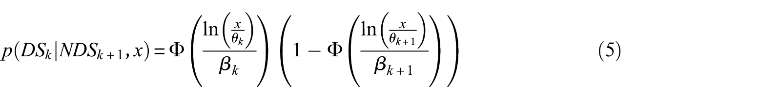
p (D S_{k} | ND S_{k + 1}, x) = Φ (\frac{\ln (\frac{x}{θ_{k}})}{β_{k}}) (1 - Φ (\frac{\ln (\frac{x}{θ_{k + 1}})}{β_{k + 1}}))

(5)

where p(DS_k|NDS_k₊₁,x) is the probability of occurrence of DS k conditional on intensity measure x and the non-occurrence of DS k+1. The MSP method stores these curves and uses two parameters of the lognormal CDF (θ_k, β_k) for each k DS, as well as a specification indicating simultaneous or exclusive DSs.

Site hazards and floor hazards

The seismic hazard at the site of a structure is defined by a frequency-intensity “site hazard curve” determined from probabilistic seismic hazard analysis and available from a national geological survey service (e.g. United States Geological Survey (USGS), 2014). The annual frequency of occurrence (f(IM)) is given by:

f (IM) = | \frac{dF (IM)}{dIM} |

(6)

where F(IM) is the annual frequency of exceedance of a ground motion intensity measure (IM).

The process for determining the hazard for a nonstructural component located at a floor level of the structure is not as well defined as for the site hazard but has received some attention in recent years. Bradley et al. (2009) and Günay and Mosalam (2013) defined the probability of exceedance of the peak floor acceleration and interstory drift ratio EDPs using total probability theorem within the PBEE methodology. Lucchini et al. (2017) and Sullivan et al. (2013) have developed approximate methods for estimating floor response spectra in linear structures. O’Reilly and Monteiro (2019) used approximate methods developed by Welch et al. (2014) for obtaining frequency-intensity EDP floor hazard curves, which provide the annual frequency of exceedance of the floor EDP for nonlinear structures. In contrast to these preceding works, the floor hazard curves used in this article are obtained from a multiple stripe analysis, defined as:

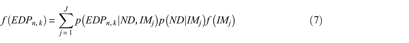
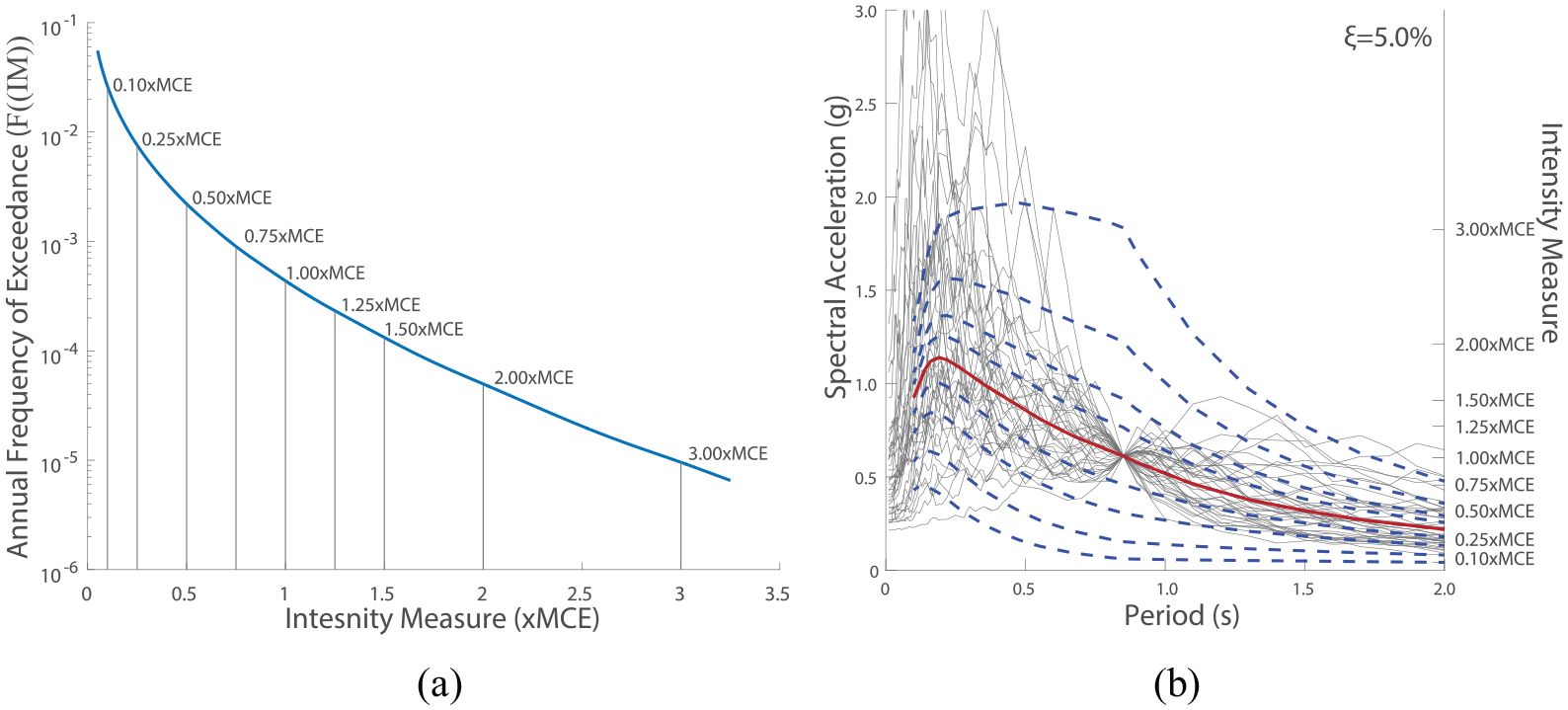
f (ED P_{n, k}) = \sum_{j = 1}^{J} p (ED P_{n, k} | ND, I M_{j}) p (ND | I M_{j}) f (I M_{j})

(7)

where f(EDP_n,k) is the annual frequency of occurrence of the EDP for the nth component’s kth DS, p(EDP_n,k|ND,IMj) is the probability of occurrence of the EDP at the jth ground motion intensity stripe conditional on non-demolition, p(ND|IM_j) is the probability of non-demolition of the building at the jth ground motion intensity stripe, and f(IM_j) is the annual frequency of occurrence of the jth ground motion intensity stripe. Figure 2 summarizes the inputs required to determine a floor hazard curve, where the EDPs obtained from the structural analysis of the building at various ground motion intensity levels are shown in Figure 2a, the probability of non-demolition is shown in Figure 2b, and the frequency of exceedance of the ground motion intensity, determined from the site hazard curve, is shown in Figure 2c.

Figure 2.

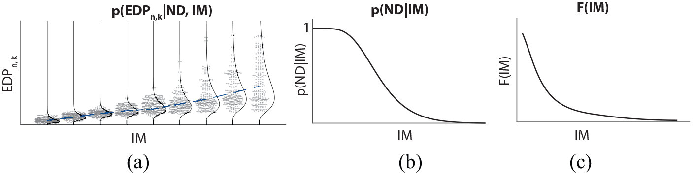
Input to the construction of a floor hazard curve (a) maximum EDP results obtained for different intensity stripes, (b) probability of non-demolition of structure, and (c) site hazard curve.

The probability of non-demolition is determined from the combined probability of non-collapse and reparable residual drifts as:

p (ND | IM) = 1 - p (D | IM) = 1 - (p (C | IM) + p (NR | NC, IM) (1 - p (C | IM)))

(8)

where p(D|IM) is the probability of demolition of the structure at a specific ground motion intensity (IM), p(C|IM) is the probability of collapse of the structure at a specific ground motion intensity (IM), and p(NR|NC,IM) is the probability of occurrence of non-reparable residual drifts at a specific ground motion intensity conditional on the non-collapse of the structure. For simplicity, the probability of demolition is taken as a function of only the residual drift in this study. While demolition may also be influenced by other considerations, such as the value of non-structural damage, including this within the formulation would create a circular relationship between Equations 7, 8, 12, and 14, as the extent of non-structural damage is a function of the frequency of floor EDP, which itself is a function of non-demolition. Furthermore, since the damage value that leads to demolition can vary widely in different contexts, it was omitted from this process. Finally, p(EDP_n,k|ND,IM_j) is the probability of occurrence of the EDP_n,k at the jth ground motion intensity conditional on non-demolition can be fitted using a lognormal probability distribution function (PDF), given as:

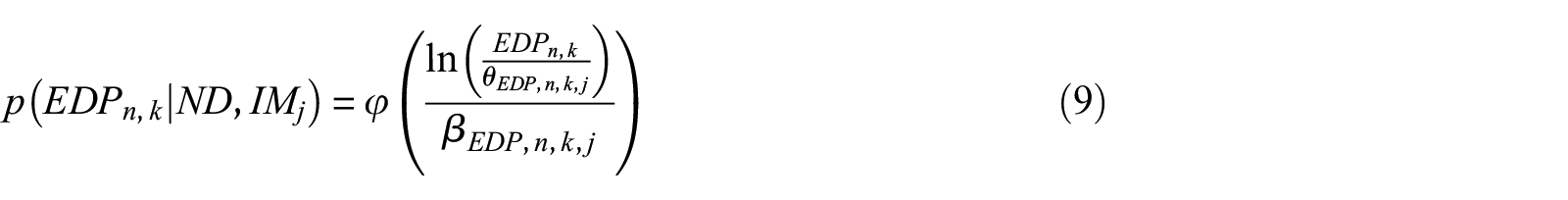
p (ED P_{n, k} | ND, I M_{j}) = φ (\frac{\ln (\frac{ED P_{n, k}}{θ_{EDP, n, k, j}})}{β_{EDP, n, k, j}})

(9)

where θ_EDP,n,k,j is the median EDP value occurring at the ground motion intensity j among non-demolished structures, and β_EDP,n,k,j is the lognormal standard deviation for the same PDF.

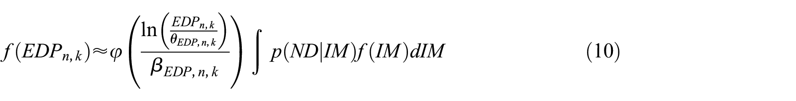
To quickly compare the change in floor hazards caused by structural upgrades, useful in the MSP method (Levels 1 and 2 of the framework in Figure 1), the f(EDP_n,k) curve is approximated using a single lognormal PDF for each EDP with parameters consisting of a median (θ_EDP,n,k) and lognormal standard deviation value (β_EDP,n,k) determined using the same MLE process as was used for the structural performance curves in the previous section. This curve is expressed as:

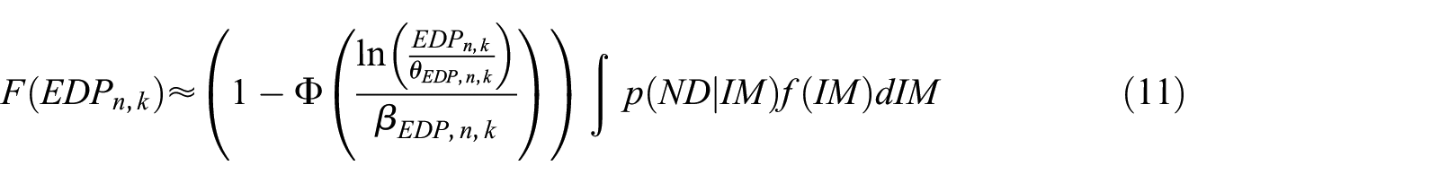
f (ED P_{n, k}) \approx φ (\frac{\ln (\frac{ED P_{n, k}}{θ_{EDP, n, k}})}{β_{EDP, n, k}}) \int p (ND | IM) f (IM) dIM

(10)

To assess the upgrade viability, values of θ_EDP,n,k and β_EDP,n,k are required for each EDP used for a fragility curve, typically consisting of peak floor interstory drifts and accelerations. The integration of Equation 10 provides the annual frequency of exceedance CDF of the EDP_n,k, providing a curve with similar properties to a site hazard curve, which is likely more familiar:

F (ED P_{n, k}) \approx (1 - Φ (\frac{\ln (\frac{ED P_{n, k}}{θ_{EDP, n, k}})}{β_{EDP, n, k}})) \int p (ND | IM) f (IM) dIM

(11)

Annual frequency of damage and mean annual loss

The EAL for a single component (or structure) n can be defined as:

EA L_{O, n} = \sum_{k = 1}^{K} (C C_{n, k}) λ (D S_{O, n, k})

(12)

EA L_{U, n} = \sum_{k = 1}^{K} (C C_{n, k}) λ (D S_{U, n, k})

(13)

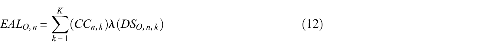
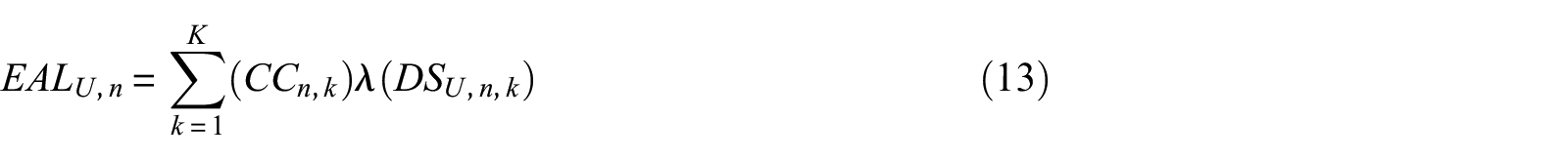
where CC_n,k is the consequence cost of DS k of component n, K is the total number of DSs considered, and λ(DS_O,n,k) and λ(DS_U,n,k) are the mean annual frequency of occurrence of the DS k of component n in its original and upgraded condition, respectively. The mean annual frequency of occurrence of damage is the integral of the function defining the annual frequency of occurrence of DS as a function of the hazard, defined as x in place of either IM for the structure or EDP for a nonstructural component:

λ (D S_{O, n, k}) = \int p (D S_{O, n, k} | x) f_{O} (x) dx

(14)

λ (D S_{U, n, k}) = \int p (D S_{U, n, k} | x) f U (x) dx

(15)

where p(DS_O,n,k|x) and p(DS_U,n,k|x) are the probabilities of occurrence of DS k of the original and upgraded component n, respectively, defined by the aforementioned fragility curves, and f_O(x) and f_U(x) are the annual frequency of occurrence of hazard (x) of the original or upgraded component, respectively.

Deaggregation of change in loss by hazard intensity

The change in mean annual frequency of occurrence of DS k of the component n can be computed from the integral of the change in the annual frequency of occurrence of damage at each hazard value x, which can be a result of a change in the probability of occurrence of damage (Δ_DS), a change in the frequency of occurrence of the hazard (Δ_H), or a change in both (Δ_DS&H). These are shown in Figure 3 and are expressed as:

Δ_{DS} (λ (D S_{n, k})) = \int Δ (p (D S_{n, k} | x)) f (x) dx'

(16)

Δ_{H} (λ (D S_{n, k})) = \int p (D S_{n, k} | x) Δ (f (x)) dx

(17)

\begin{matrix} Δ_{D S & H} (λ (D S_{n, k})) = \int^{} (Δ p (D S_{n, k} | x) f_{O} (x) + p (D S_{O, n, k} | x) Δ (f (x)) - \\ Δ (p (D S_{n, k} | x)) Δ (f (x))) d x \end{matrix}

(18)

Figure 3.

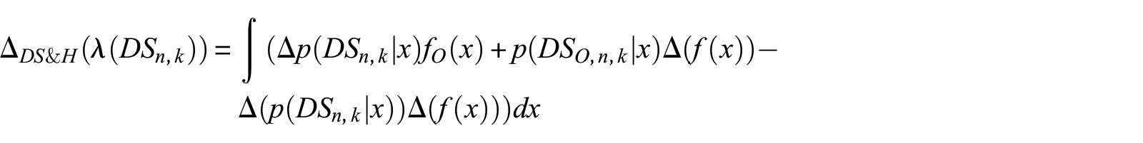
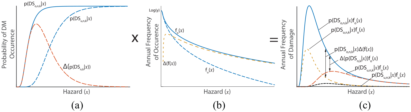
(a) Change in probability of damage state occurrence, (b) change in frequency of exceedance of hazard, and (c) change in annual frequency of occurrence of damage.

A particularly useful application of the deaggregation of change in damage functions shown above is when determining the BCR of the upgrade of a component whose upgrade has no other effects on the overall building loss, as when determining the viability of an individual nonstructural component upgrade in a structure with a given floor hazard curve. In these simplified cases, Equation 16 can be substituted into Equation 2 to define the BCR of component n as a function of hazard intensity (bcr_n(EDP_n,k)):

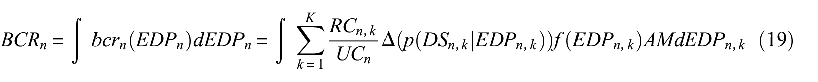
BC R_{n} = \int bc r_{n} (ED P_{n}) dED P_{n} = \int \sum_{k = 1}^{K} \frac{R C_{n, k}}{U C_{n}} Δ (p (D S_{n, k} | ED P_{n, k})) f (ED P_{n, k}) AMdED P_{n, k}

(19)

Equation 19 can be used to identify the hazard values where the change in component performance provided by the component upgrade has the largest benefit, and inversely, the hazard values where performance improvements would have the greatest influence.

Deaggregation of the influence of upgrades on losses

To quickly assess the upgrade viability, it is convenient to evaluate the change in EAL from an upgrade strategy across four categories: (1) change in loss caused by the changes to the collapse fragility of the structure, (2) change in loss caused by changes to the probability of demolition of the structure due to non-reparable residual drifts, (3) change in loss caused by changes to the floor EDPs that impact the nonstructural components, and (4) change in loss caused by changes to the nonstructural component fragilities. Each of these is characterized below.

Influence of changes to the collapse fragility of the structure

To quantify the change in annual frequency of collapse caused by modifications to the structural performance, the parameters of the lognormal CDFs of the original and upgraded collapse curves are required. Also using the site hazard curve (f(IM)), this change in annual frequency of occurrence is expressed as:

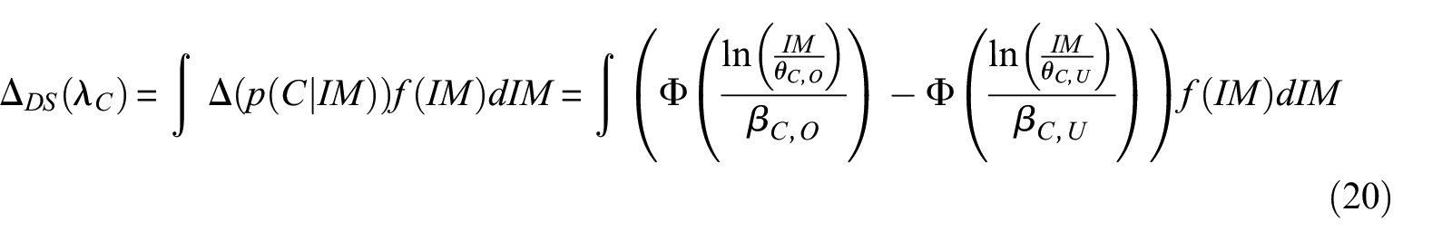
Δ_{DS} (λ_{C}) = \int Δ (p (C | IM)) f (IM) dIM = \int (Φ (\frac{\ln (\frac{IM}{θ_{C, O}})}{β_{C, O}}) - Φ (\frac{\ln (\frac{IM}{θ_{C, U}})}{β_{C, U}})) f (IM) dIM

(20)

where Δ_DS(λ_C) is the change in mean annual frequency of collapse caused by a change in structural performance, θ_C,O and θ_C,U are the median collapse intensity measure values for the original and upgraded structure, respectively, and β_C,O and β_C,U are the lognormal standard deviation of the collapse lognormal CDF of the original and upgraded structure, respectively.

The consequence cost of collapse is a combination of the building replacement value (BV) and the loss from the average number of casualties caused by collapse, which can be obtained using an equivalent continuous occupancy approximation (Comerio, 2000):

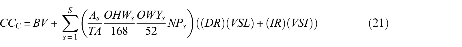
C C_{C} = BV + \sum_{s = 1}^{S} (\frac{A_{s}}{TA} \frac{OH W_{s}}{168} \frac{OW Y_{s}}{52} N P_{s}) ((DR) (VSL) + (IR) (VSI))

(21)

where BV is the building replacement value; A_s is the area of a specific occupancy type (s); TA is the total area of the building; OHW_s is the occupied hours per week for an average building occupant of occupancy type (s); OWY_s is the occupied weeks per year for an average building occupant of occupancy type (s); NP_s is the maximum number of occupants in the building of occupancy type (s); DR and IR are the death rate and injury rate per occupant, respectively; and VSL and VSI are the value of a statistical life and value of a statistical injury, respectively. Values for each of these variables can be obtained from a variety of sources (Department of Homeland Security (DHS)/Federal Emergency Management Agency (FEMA), 2007; United States Department of Transportation (DOT), 2016), or using information provided by the building owner. This results in the change to the EAL contributed by the collapse of the structure to be:

Δ (EA L_{C}) = C C_{C} (Δ_{DS} (λ_{C}))

(22)

The changes in EAL_C resulting from changes to the lognormal fragility curve defining structural collapse can be summarized by the change (ratio) in both the median (Q_θ,C) and lognormal standard deviation (Q_β,C) of the original to the upgraded curve, as shown:

Q_{θ, C} = \frac{θ_{C, U}}{θ_{C, O}}

(23)

Q_{β, C} = \frac{β_{C, U}}{β_{C, O}}

(24)

Since structural upgrades are not expected to cause large changes in β_C (FEMA, 2018; Liel et al., 2009), most of the change in EAL_C can be captured by Q_θ,C.

Influence of changes to non-reparable residual drift fragility of the structure

Similar to changes in collapse performance, the change in loss caused by non-reparable residual drifts resulting from a structural upgrade can be expressed as:

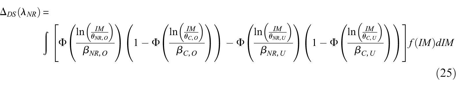
Δ_{D S} (λ_{N R}) = \int^{} [Φ (\frac{\ln (\frac{I M}{θ_{N R, O}})}{β_{N R, O}}) (1 - Φ (\frac{\ln (\frac{I M}{θ_{C, O}})}{β_{C, O}})) - Φ (\frac{\ln (\frac{I M}{θ_{N R, U}})}{β_{N R, U}}) (1 - Φ (\frac{\ln (\frac{I M}{θ_{C, U}})}{β_{C, U}}))] f (I M) d I M

(25)

where Δ_DS(λ_NR) is the change in mean annual frequency of occurrence of non-reparable residual drifts from a change in performance, θ_NR,O and θ_NR,U are the median non-reparable residual drifts intensity measures for the original and upgraded structure, respectively, and β_NR,O and β_NR,U are the lognormal standard deviation of the non-reparable residual drift lognormal CDF of the original and upgraded structure, respectively. A building with non-reparable residual drifts is assumed for simplicity not to have caused any casualties, the consequence cost for this DS is simply the building value, and thus the change in EAL is given by:

Δ (EA L_{NR}) = BV \int Δ (p (NR | IM)) f (IM) dIM

(26)

Similar to the representation of the change in EAL_C using Q_θ,C, the change in EAL_NR can be captured using Q_θ,NR and Q_β,NR, where Q_θ,NR is the change in median non-reparable residual drifts intensity value and Q_β,NR is the change in lognormal standard deviation non-reparable residual drifts intensity value, given by:

Q_{θ, NR} = \frac{θ_{NR, U}}{θ_{NR, O}}

(27)

Q_{β, NR} = \frac{β_{NR, U}}{β_{NR, O}}

(28)

Influence of changes to the floor hazard

Upgrades to the structural system can modify the dynamic properties of the structure, resulting in changes to the losses caused by damage to both nonstructural and reparable structural components. Since the MLE method was used to define the floor hazard curves using a lognormal distribution, as discussed in the “Hazards” subsection, the change in annual frequency of occurrence of a DS k of a component n as a function of the change in corresponding EDP is expressed as:

Δ_{H} (λ_{n, k}) = \int p (D S_{n, k} | ED P_{n, k}) Δ (f (ED P_{n, k})) dED P_{n, k}

(29)

Δ (f (E D P_{n, k})) = φ (\frac{\ln (\frac{E D P_{n, k}}{θ_{E D P, n, k, O}})}{β_{E D P, n, k, O}}) \int^{} p (N D_{O} | I M) f (I M) d I M - φ (\frac{\ln (\frac{E D P_{n, k}}{θ_{E D P, n, k, U}})}{β_{E D P, n, k U}}) \int^{} p (N D_{U} | I M) f (I M) d I M

(30)

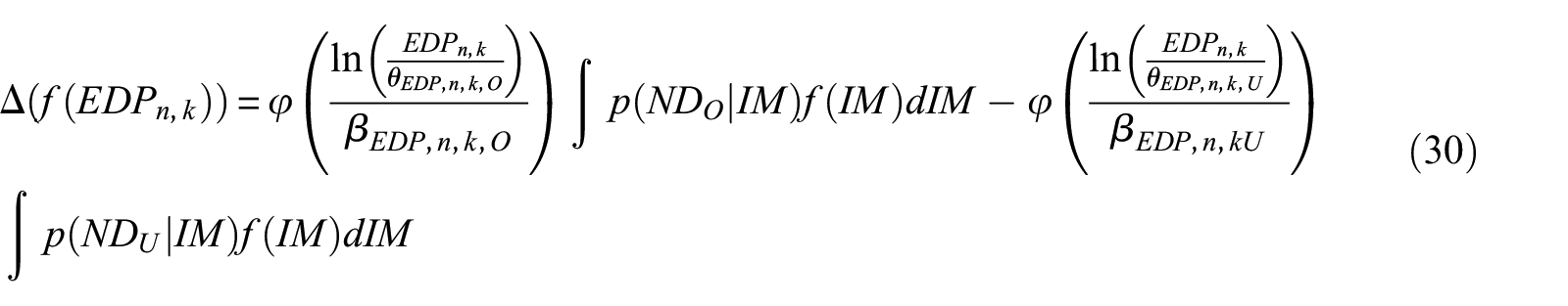
where Δ_H(λ_n,k) is the change in median annual frequency of occurrence of the kth DS of the nth component from a change in floor hazard; φ is the standard Gaussian PDF; p(ND_O|IM) and p(ND_U|IM) are the probability of non-demolition of the original and upgraded structure, respectively; θ_EDP,n,k,O and θ_EDP,n,k,U are the original and upgraded median EDP values of the floor hazard curves, respectively; and β_EDP,n,k,O and β_EDP,n,k,U are the lognormal standard deviation of the original and upgraded floor hazard curves, respectively. The consequence cost associated with each of these changes is the repair cost (RC) associated with the kth DS of the nth component, and thus the total change to the EAL caused by a structural upgrade can be defined by the summation of the change in annual loss across all components N, expressed as:

Δ_{H} (EA L_{NS}) = \sum_{n = 1}^{N} \sum_{k = 1}^{K} R C_{n, k} Δ_{H} (λ_{n, k})

(31)

Similar to the change in EAL_C and EAL_R, the change in EAL_NS of either acceleration or displacement sensitive nonstructural components from a change in their respective EDP floor hazard curves can be expressed by Q_θ,EDP,n,k and Q_β,EDP,n,k factors given by:

Q_{θ, EDP, n, k} = \frac{θ_{EDP, n, k, U}}{θ_{EDP, n, k, O}}

(32)

Q_{β, EDP, n, k} = \frac{β_{EDP, n, k, U}}{β_{EDP, n, k, O}}

(33)

Casualties caused by nonstructural components occurring outside of the building enveloped were not explicitly considered in the application of this methodology. However, if sufficient information about the occupancy type of the surrounding area is provided, a modification to the RC of a component could be introduced to capture this effect, similar to the consequence cost of collapse (CC) determined in Equation 21.

Influence of changes to the fragility of nonstructural components

The change in loss caused by an improvement to the performance of a nonstructural component $Δ_{DS} (λ_{n, k})$ can be expressed as:

Δ_{DS} (λ_{n, k}) = \int (p (D S_{O, n, k} | ED P_{n, k}) - p (D S_{U, n, k} | ED P_{n, k})) f (ED P_{n, k}) dED P_{n, k}

(34)

Equation 34 can be used when contemplating an upgrade strategy limited only to the nonstructural components, which will not modify the dynamic behavior of the structure. This is shown in Equation 35 as:

Δ (EA L_{NS only}) = \sum_{n = 1}^{N} \sum_{k = 1}^{K} R C_{n, k} Δ_{DS} (λ_{n, k})

(35)

However, when considering an upgrade strategy that includes both structural and nonstructural components, the possibility of simultaneous changes to the component performance and to the floor hazard $Δ_{DS ambasend H} (λ_{n, k})$ must be considered by:

\begin{matrix} Δ_{D S & H} (λ_{n, k}) = \int^{} (p (D S_{O, n, k} | E D P_{n, k}) Δ (f (E D P_{n, k})) + Δ (p (D S_{n, k} | E D P_{n, k})) f_{O} (E D P_{n, k}) \\ - Δ (p (D S_{n, k} | E D P_{n, k})) Δ (f (E D P_{n, k}))) d E D P_{n, k} \end{matrix}

(36)

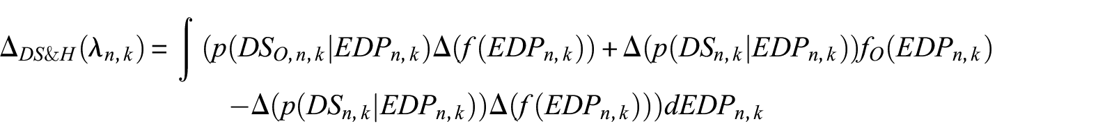
Thus, the change in EAL from nonstructural component damage when including both structural and nonstructural upgrades becomes:

Δ (EA L_{NS}) = \sum_{n = 1}^{N} \sum_{k = 1}^{K} R C_{n, k} Δ_{DS ambasend H} (λ_{n, k})

(37)

Discussion of framework levels

As mentioned in the “Overview” section, the use of multiple levels in the framework for assessing upgrade viability allows for increasing analytical accuracy by differing loss estimation analysis methods. The lower effort associated with the first two levels of the framework requires the organization of the equations outlined in the previous section into the MSP method, which quickly quantifies the approximate effect of a structural upgrade on the expected losses. This MSP method is explained in greater detail in this section, and aspects of this method are compared to the Level 3 PBEE Monte Carlo optimization.

Level 1: MSP method for feasibility study of upgrade strategy

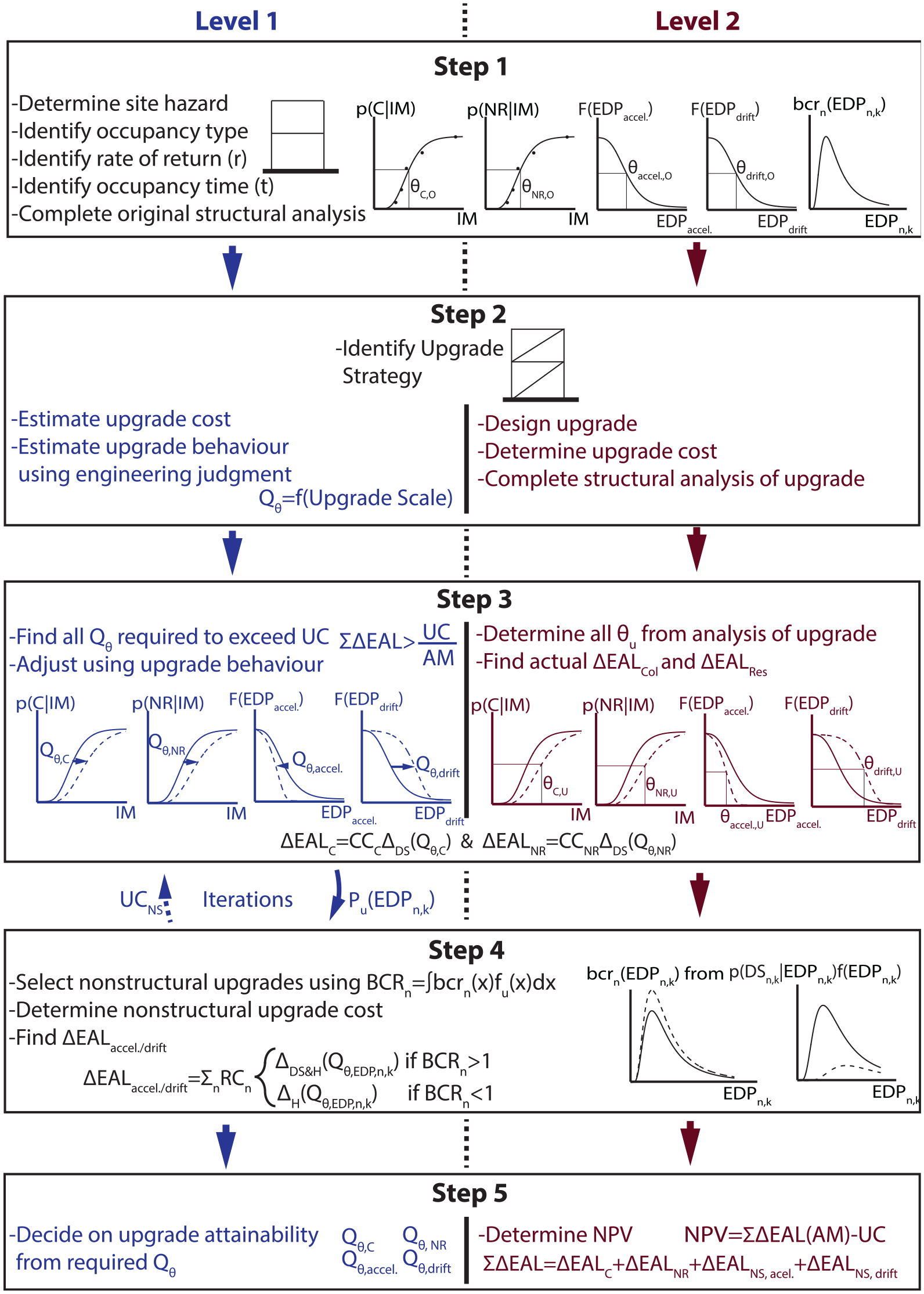
Both Levels 1 and 2 assessments use the MSP method to determine the viability of an upgrade strategy. The MSP method is structured to allow for the rapid initial estimation of the impact of structural modifications on various sources of loss. This relies on the assumption that the seismic structural responses presented as key parameters of the MSP method are lognormally distributed and uses the deaggregated changes in the performance curves presented in the “Deaggregation of change in loss by hazard intensity” section. While the MSP method used in Level 1 or Level 2 assessments is identical, as shown in Figure 4, the objective of the analysis and the quality of data used for each level differ. For a Level 1 analysis, the MSP method includes the following steps:

Identify original building conditions including structural system, nonstructural population, owner parameters, and site hazard to determine θ and β values for collapse, residual drift, and floor hazard curves for the original structure.

Select an upgrade strategy, estimate whether each associated Q_θ is greater than or less than one, and approximate the structural upgrade cost as a fraction of the building value.

Determine the required Q_θ value for each performance curve to obtain the required change in EAL, using Equations 20 to 23 for collapse and Equations 25 to 27 for non-reparable residual drift.

Identify the nonstructural components to upgrade by using Equation 19 with the updated floor hazard curve, adjusted with the Q_θ value for each EDP. Update the upgrade cost in Step 3 as needed and continue modifying the Q_θ values and the selection of nonstructural upgrades until the required change in EAL is obtained, determined using Equations 29 to 37 for nonstructural components, as applicable.

Estimate if the final Q_θ values are attainable with the proposed upgrade strategy.

Figure 4.

Flow chart for Levels 1 and 2 of MSP method of assessment of upgrade viability.

While it is recommended that the θ and β values for the collapse and residual drift curves in Step 1 be determined based on a nonlinear time history analysis (NLTHA), approximate methods to determine the collapse performance of a structure are available (Chopra, 2012; Moon et al., 2012) and could be used in a Level 1 type analysis. Similarly, θ and β for the floor hazard curve can either be fitted from NLTHA results or by using various approximate methods (Merino et al., 2019; O’Reilly and Calvi, 2020; Sullivan et al., 2014; Welch et al., 2014). A tool implemented in Microsoft Excel has been developed to quickly iterate between Steps 3 and 4 of the method and is included as a supplementary file to this article.

Level 2: MSP method for verification of schematic design of upgrade strategy

If the obtained Q_θ values for the upgrade strategy have been deemed achievable in the Level 1 of the MSP method, the use of more resource-intensive tools can be justified to determine the viability of the upgrade strategy in a Level 2 analysis. The verification of viability is completed using the same MSP method, but replacing the approximations in Step 2 with more detailed cost estimates and the results in Step 3 from an NLTHA. The steps for this method are summarized as follows:

Same step as in Level 1 but potentially utilizing more accurate models to determine θ and β values.

Design structural upgrade, obtain structural upgrade cost estimate, and perform NLTHA.

Determine actual curve parameters (θ and β) for the upgraded structure to determine change in collapse and non-reparable residual deformation EALs.

Determine nonstructural component upgrades using floor hazard curves obtained from NLTHA and determine change in nonstructural EAL.

Find NPV from Equation 1 using both the structural and nonstructural upgrade costs.

Level 3: optimization using Monte Carlo PBEE evaluation

The goal of a Level 3 analysis is to apply an end-to-end scenario-based PBEE method to further verify and optimize the upgrade strategies beyond the components identified using the MSP method in the Level 2 analysis. The GA in the study by Steneker et al. (2020), used to optimize the seismic upgrade of a building using the Monte Carlo–based PBEE method, is an example of a Level 3 analysis. The Monte Carlo scenario evaluation allows for the inclusion of several factors not considered in the MSP method, as discussed next.

First, by simultaneously considering all components selected for upgrade when determining the overall upgrade cost, the individual cost of the component upgrades can be reduced by identifying common tasks. Furthermore, as the Monte Carlo approach typically subdivides each component quantity into multiple subdivisions evaluated independently, the ability to capture both shared consequence functions across components and to determine economies-of-scale cost reductions is possible in Level 3. These are not reflected in the MSP method of the Level 2 analysis, as the EAL and BCR of all individual nonstructural components are evaluated with a single function for the entire component quantity. An iterative version of the MSP method (MSPIT) is introduced in the case study example to attempt to overcome this shortcoming of the MSP method, and is discussed further in this article.

Second, since the GA developed by Steneker et al. (2020) used a Monte Carlo implementation of PBEE, the consequence function and upgrade cost were defined using probabilistic distributions that captured variability in repair and upgrade costs. This factor, in combination with the randomness of the GA selection process, results in variation in the final optimal upgrade solution, as components with BCR values close to one are selected in a fraction of the repeated iterations. To identify these components, the optimization run is repeated several times, and the rate at which components are selected in the optimal solution at each value is recorded. In contrast, the MSP method produces a single deterministic selection of components in the optimal upgrade strategy.

Case study example

The case study example used to demonstrate the framework described above is the same scenario considered by Steneker et al. (2020) to illustrate a Level 3 analysis with GA. This section focuses on the implementation of Level 1 and Level 2 analyses, while results from the Level 3 analysis are summarized to allow comparisons.

Level 1 analysis

Step 1: original conditions

The original archetype structure is a three-story steel moment-resisting frame (MRF) with an office type occupancy, located in Seattle, Washington, on site class B soil. The owner profile used for the analysis is assumed to have a 2% rate of return and 40-year occupancy time, representative of a typical institutional building owner (Shilling and Wurtzebach, 2018). The population of nonstructural components included in this archetype structure consists of all 26 components identified by the FEMA P-58 Normative Quantity Tool (FEMA, 2018). The structure was designed according to the seismic provisions of the 1994 Uniform Building Code (UBC, 1994) and, with the exception of pre-Northridge Earthquake beam-to-column connections, satisfies current seismic design requirements (American Institute of Steel Construction (AISC), 2016). Plan and elevation views for this frame are shown in Figure 5. The building was assumed to have no torsional irregularities. The frame model for both the MSP method Level 1 and Level 2 analysis of this original structure was assembled in OpenSees (McKenna et al., 2000), with concentrated zero-length springs capturing element nonlinearity using the Ibarra–Medina–Krawinkler hysteretic model (Ibarra et al., 2005). The nonlinear behavior of the panel zones was also modeled using the Krawinkler Spring Box model with a trilinear backbone curve (Gupta and Krawinkler, 1999). The computed fundamental period of the frame was 0.87 s. Details of the modeling of the archetype structure are provided by Steneker (2020).

Figure 5.

(a) Plan view of archetype building and (b) elevation view of archetype building with modeling details.

The seismic hazard analysis for the archetype building’s site was obtained using the USGS Uniform Hazard Tool (USGS, 2014). A frequency–intensity curve was obtained for the original structure’s fundamental period, as shown in Figure 6a. A multiple stripe analysis (Baker, 2015) was used to evaluate the structural performance of the frame, with nine intensity stripes, each with 40 ground motions selected and scaled to match different conditional mean spectra (Baker and Lee, 2017). For each stripe, ground motions were selected from the far-field NGA-West2 Database (PEER Center, 2013) to match rupture parameters identified by the site seismic hazard deaggregation information corresponding to the frequency of occurrence of each stripe’s intensity. Details on the ground motion selection is provided by Steneker (2020).

Figure 6.

(a) Archetype building’s site frequency–intensity curve and (b) conditional mean spectra for multiple stripe analysis.

The results of the multiple stripe analysis were represented by five lognormal CDFs whose parameters were determined using the MLE method. The fragility curves for collapse and for non-reparable residual drifts conditional on non-collapse are shown in Figure 7a. The probability of building demolition, p(D|IM), and the probability of non-reparable residual drifts are also included. Figure 7b shows the peak floor and roof acceleration hazard curves and includes the values obtained directly from the NLTHA results, as well as the approximate lognormal CDF fitted to the NLTHA results using the MLE method. Two acceleration curves were used since the floor and roof levels have different populations of nonstructural components. The distinctive drops in values of the acceleration hazard curves in Figure 7b are caused by the increasing probability of demolition of the original building at larger intensity stripes. Finally, Figure 7c shows the floor hazard curve for the peak interstory drifts before collapse. In all instances, the assumption of lognormality of the floor hazards obtained from the sample of NLTHA at all intensities passed the one-sample Kolmogorov–Smirnov test having an alpha value of 5% (Chakravarti et al., 1967).

Figure 7.

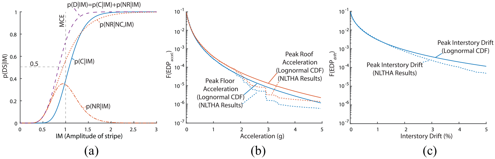
Performance curves for original structure (a) structural fragility curves, (b) roof and floor acceleration hazard curves, and (c) floor drift hazard curve.

Step 2: upgrade cost and structural behavior

This case study example considered three structural upgrade strategies of the archetype building and one strategy that limited upgrades to the nonstructural components only. All three structural strategies are commonly recommended in practice for steel MRFs with pre-Northridge connections (ASCE, 2017; FEMA, 2000). A short description of the assumed effect of each strategy on the four loss categories is provided below and an estimate of cost is listed in Table 1. This step required the most assumptions in Level 1 of the MSP method, and a more accurate estimation of cost and behavior is considered in Level 2.

Table 1.

Summary of upgrade strategies and assumed Q_θ values for Level 1 of MSP method

Upgrade strategy	Structural cost estimate(% of BV)	Structural and nonstructural cost estimate (% of BV)	Collapse Q_θ	Residual drift Q_θ	Flooracceleration Q_θ	Floordrift Q_θ
1. Increase in strength and stiffness	5	11	1.4	1.2	1.4	0.4
2. Increase in ductility/self-centering	10	14	1.6	1.8	1.1	1.1
3. Addition of supplemental viscous damping	15	17	1.0	1.0	0.7	0.8
4. Upgrade of nonstructural components	0	6.6	1.0	1.0	1.0	1.0

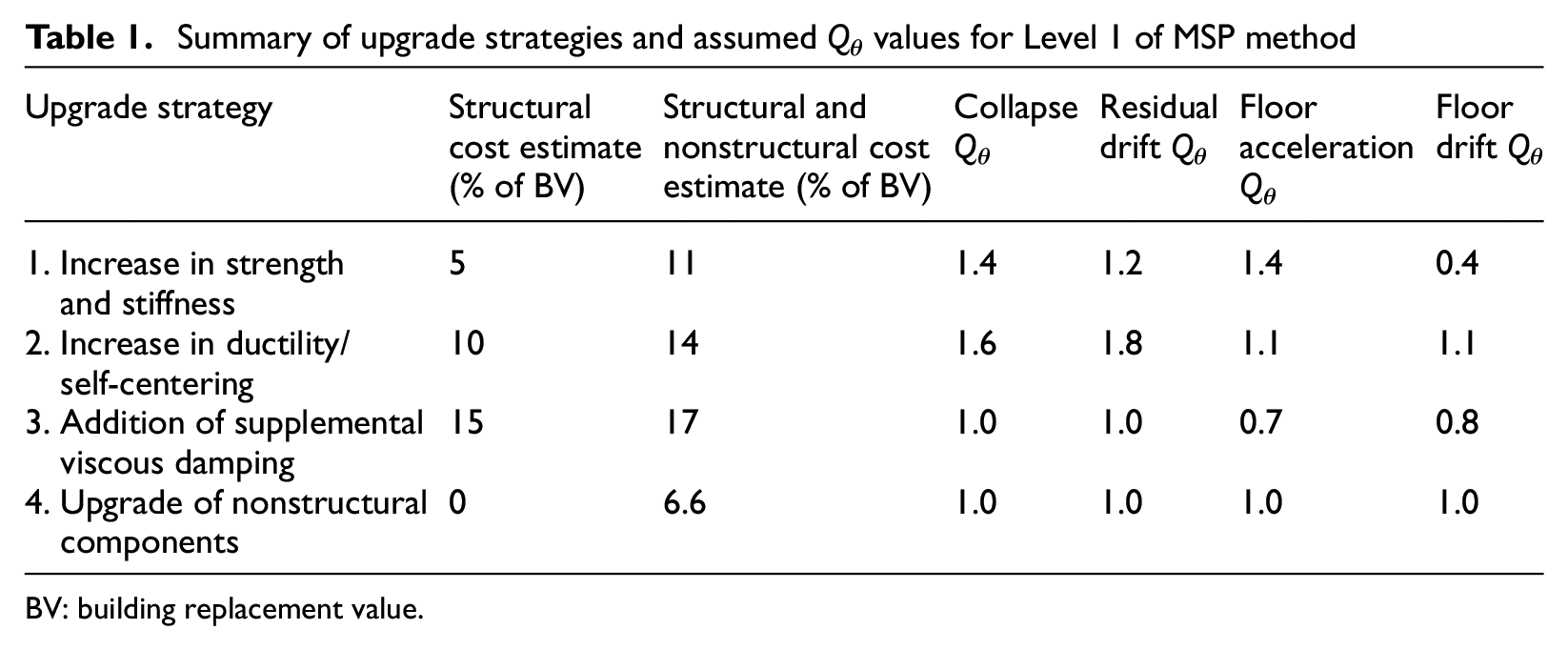
BV: building replacement value.

Structural upgrade strategy 1: Increase strength and stiffness. This strategy is typically achieved with the addition of seismic force-resisting elements, such as braces. The main objectives of this strategy are to increase collapse resistance and reduced residual drifts. This characteristic also typically results in smaller interstory drifts but higher floor accelerations (Flores et al., 2015; Mayes et al., 2013).

Structural upgrade strategy 2: Increase ductility and/or self-centering. This strategy is typically achieved by modifying the beam–column connections to provide greater displacement capacity. This strategy increases the collapse resistance and may reduce residual drifts. However, the increase in the probability of non-demolition at higher ground motion intensities also increases the frequency of occurrence of both large accelerations and interstory drift EDPs (Steneker et al., 2021; Yeow et al., 2018).

Structural upgrade strategy 3: Addition of supplemental viscous damping. This strategy is typically achieved with the addition of viscous dampers (VDs). This strategy increases the collapse resistance and may reduce residual drifts. The addition of VDs s usually also reduces both interstory drifts and floor accelerations (Mayes et al., 2013).

Structural upgrade strategy 4: Upgrades to nonstructural components. This strategy consists of upgrading all nonstructural components with a BCR_n value larger than one (Equation 19) in the original structural condition. The strategy was not considered to change any of the Q_θ values but still reduced the EAL.

Steps 3 and 4: required change in EAL and approximation of Q_θ values

A required minimum change in EAL was determined based on the estimated upgrade cost for each strategy and the amortization value obtained for the building owner profile. The changes in EAL obtained from shifts in Q_θ value were evaluated using Equations 20 to 23 for collapse and Equations 25 to 27 for non-reparable residual drifts. Each shift in Q_θ values for either the floor acceleration (PFA) or floor interstory drift EDPs in Equation 32 was considered in Step 4 to determine all accompanying nonstructural component upgrades, and any modification in upgrade cost of these components was included in the upgrade cost used in Step 3 through an iterative process. Table 1 lists all the Q_θ values assumed in Level 1 of the MSP method based on engineering judgment. Using the Excel tool provided in Appendix A in Supplementary Material of this article, a nonstructural component n was upgraded when the integral of the product of bcr_n(EDP) from Equation 19 and the upgraded floor hazard resulting from the Q_θ value Δ(f(EDP_n,k)) exceeded 1, leading to the change in EAL for component n being evaluated using Equation 36 instead of Equation 29. The relevant nonstructural repair (RC_n) and upgrade costs (UC_n) used in Equation 19 are summarized in Table 2 as a fraction of the total building value for all 26 component types. The nonstructural upgrades followed the FEMA E-74 guidelines (FEMA, 2012) and the upgrade costing was determined using the RSMeans commercial software estimating tools (RSMeans, 2018). The iterative process was completed once the total change in EAL exceeded the upgrade cost divided by the amortization conversion.

Table 2.

Summary of nonstructural normalized repair and upgrade costs for case study structure

Component (n)	Quantity (unit)	Demand parameter	Source offragilityfunction	Consequence function	$R C_{n}$ (% of BV)	Upgrade	UC_n (% of BV)
Chiller	1300 Ton	PRA (g)	FEMA P-58	Replacement	11.00	Reseating on seismic snubbers	1.48
Cooling tower	1300 Ton	PRA (g)	FEMA P-58	Replacement	11.00	Reseating on seismic snubbers	1.48
Air handling unit	12,800 CFM	PRA (g)	FEMA P-58	Repair attaching ducts	0.40	Installation of flexible coupling	1.04
				Replacement	15.00	Reseating on seismic snubbers	1.03
Motor controller	13 units	PRA (g)	FEMA P-58	Replacement	0.40	Proper anchorage	0.11
Low voltage transformer	6 units	PRA (g)	FEMA P-58	Replacement	1.50	Proper anchorage	0.07
Distribution panel	3 units	PRA (g)	FEMA P-58	Replacement	0.70	Proper anchorage	0.07
Control panel	5 units	PRA (g)	FEMA P-58	Replacement	0.15	Proper anchorage	0.10
Lighting	1900 units	PFA (g)	FEMA P-58	Replacement	13.5	Safety cable	1.00
Desktop equipment	450 units	PFA (g)	FEMA P-58	Replacement	4.78	Proper anchorage	1.10
Office furniture	450 units	PFA (g)	Filiatraultet al. (2004)	Replacement	4.78	Proper anchorage	0.81
Large HVAC duct	1285 LF	PFA (g)	FEMA P-58	Repair support	0.02	Installation of bracing or trapeze	0.58
				Replace section	0.22
Small HVAC duct	4815 LF	PFA (g)	FEMA P-58	Repair support	0.05	Installation of bracing or trapeze	0.73
				Replace section	0.60
HVAC diffuser	580 units	PFA (g)	FEMA P-58	Replacement	1.35	Safety wires	1.33
Cold piping	5390 LF	PFA (g)	FEMA P-58	Repair	0.16	Installation of bracing or trapeze	0.61
				Replace (flooding)	5.05
Large diameter piping	1925 LF	PFA (g)	FEMA P-58	Repair	0.10	Installation of bracing or trapeze	0.50
				Replace (flooding)	1.84
Small diameter piping	5390 LF	PFA (g)	FEMA P-58	Repair	0.16	Installation of bracing or trapeze	0.90
				Replace (flooding)	5.05
Sanitary piping	3660 LF	PFA (g)	FEMA P-58	Replace (flooding)	3.50	Installation of bracing	0.71
Sprinkler piping	12,840 LF	PFA (g)	Soroushianet al. (2015)	Repair	0.26	Installation of bracing or trapeze	1.54
				Replace (flooding)	12.00
Sprinkler head	580 units	PFA (g)	Soroushianet al. (2015)	Repair	0.02	Installation of flexible piping	1.04
				Replace (flooding)	0.30
				Replace (flooding)	5.27
Suspended ceiling	57,780 SF	PFA (g)	FEMA P-58	Repair 5%	0.71	Installation of wire bracing, cross runners	5.04
				Repair 30%	5.57
				Repair 100%	11.50
Raised floor	481 SF	PFA (g)	FEMA P-58	Repair	0.47	Pedestal bracing	0.28
Curtain glazing	19,260 SF	Drift (%)	Behr (1998)	Replace cracked glass	10.00	Replace with shatter proof glass	6.80
				Replace broken glass	10.00
Wall partitions	6420 LF	Drift (%)	Retamaleset al. (2013)	Re-tape joints	1.55	Partial height, Installation of lateral bracing	3.16
				Replace 10%	3.10
				Replace 50%	4.77
Roofing tiles	21850	PRA (g)	FEMA P-58	Minor reinstall	3.70	Installation of veneer anchor	4.48
				Major reinstall	10.10
Concrete stairs	24 units	Drift (%)	Bull (2011)	Repair cracks	0.17	Installation of proper seismic joint at landing	1.16
				Major repair	0.92
				Replacement	6.78
Elevator	6 units	PRA (g)/PFA (g)	FEMA P-58	Repair controls	0.37	Proper anchorage of rails and equipment	0.56
				Repair rails	1.59
				Repair car	0.21

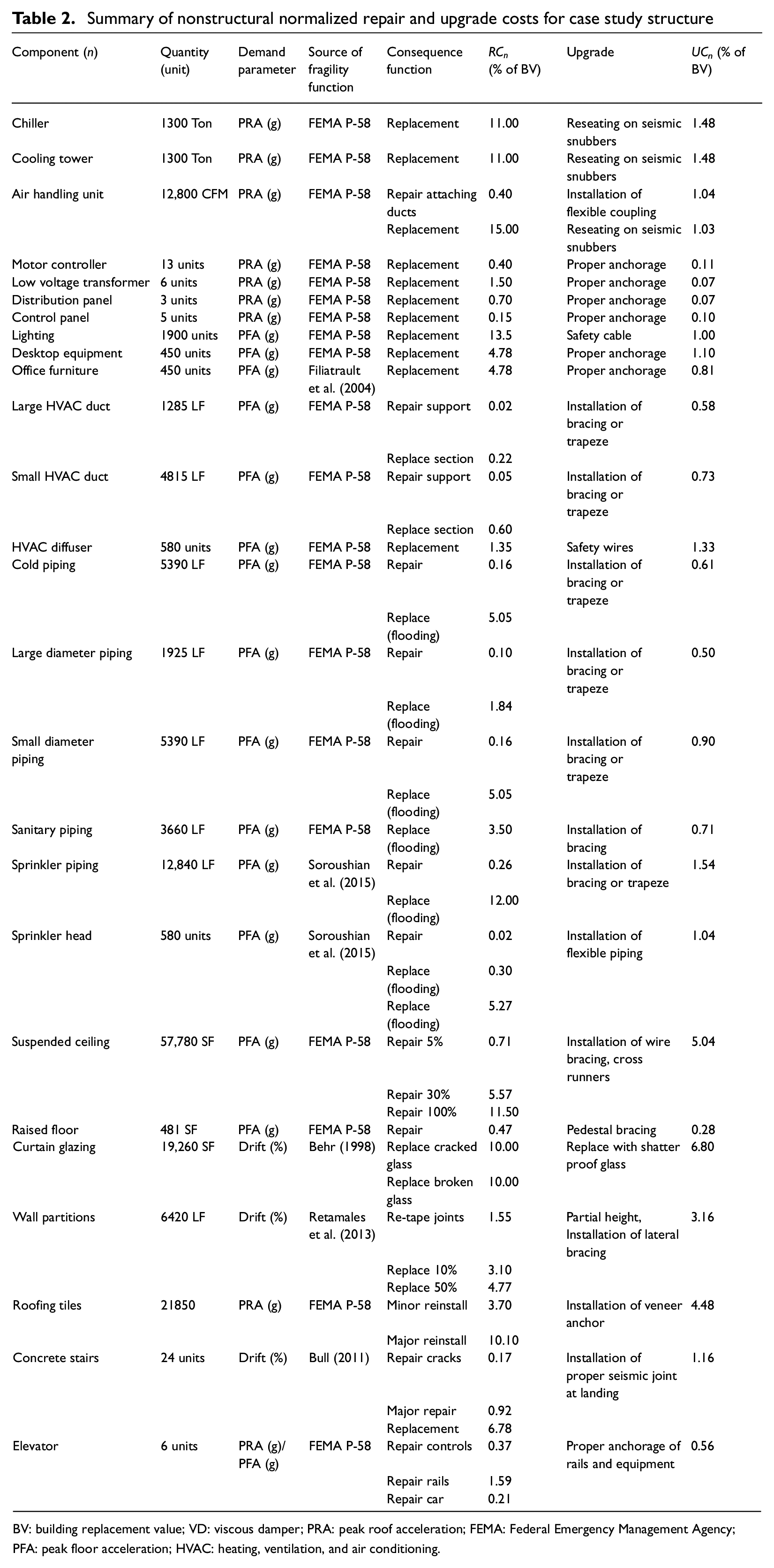
BV: building replacement value; VD: viscous damper; PRA: peak roof acceleration; FEMA: Federal Emergency Management Agency; PFA: peak floor acceleration; HVAC: heating, ventilation, and air conditioning.

Step 5: determination of attainability of Q_θ values

Relevant engineering experience and further research would have provided more accurate guidance on estimating Q_θ for each upgrade strategy. Owner profiles with shorter occupancy times and higher rates of return lead to a need for larger Q_θ values for a viable retrofit, which would be deemed less attainable. However, in this case study, the values shown in Table 1 were all considered achievable based on engineering judgment, so each upgrade strategy was considered for a Level 2 analysis.

Level 2 analysis

Step 1: original conditions

Since a detailed model of the original building was used in the Level 1 analysis, the same model was used for the Level 2 analysis. No further refinement of the numerical results was required.

Step 2: upgrade design, cost, and performance

The increase in stiffness and strength was implemented using the installation of buckling restrained braces (BRBs) in the MRFs. The design process for the BRB structural upgrade used an iterative implementation of the equivalent lateral force procedure as outlined in ASCE 7-16, where the design period of the structure was determined from modal analysis of the combined MRF/BRB system, but with the BRBs designed to take 100% of the lateral loads. The increase in ductility and the addition of self-centering behavior was implemented by replacing the pre-Northridge connections with low-damage self-centering sliding hinge joint (SCSHJ) connections (Khoo et al., 2012) without changing the beam section. The design of the SCSHJ connections targeted 100% self-centering capability in each beam–column connection, and the activation moment was set to allow for the full connection mechanism to develop before yielding of the existing beam (Steneker, 2020). The addition of supplemental damping was realized using diagonal linear VDs that were designed to provide either 10% or 25% damping in the first mode of the structure using the process outlined by Christopoulos and Filiatrault (2006). In both the 10% and 25% VD designs, the number of dampers in each frame was minimized to provide the required damping level, but the size of the dampers was limited to avoid yielding in adjacent original structural elements. The implementation of all structural upgrades, with the exception of the BRBs, was also considered with the possibility of an incremental floor implementation where the upgrades was installed at only the first floor, or only the first two floors, or at all three floors. Since the installation of the BRBs at only a limited number of floors would cause a vertical stiffness and strength irregularity, its implementation at a subset of floors was not considered. The design details for each upgrade option for a single frame of the structure are presented by Steneker (2020), and the estimated costs for all 10 structural upgrade options are summarized in Table 3.

Table 3.

Summary of structural repair and upgrade costs for Level 2 of MSP method

Component (n)	Quantity (unit)	Demand parameter	Source of fragilityfunction	Consequence function	$R C_{n}$ (% of BV)	Upgrade	UC_n (% of BV)
Total building	1 unit	Drift (%)	Structuralanalysis	Building replacement and casualties	100 + 250	1, 2, and 3 BRB	6.6
						1 10% VD	7.9
						1 and 2 10% VD	8.9
						1, 2, and 3 10% VD	10.5
		Residual drift (%)	Structural analysis	Building replacement	100	1 25% VD	7.5
						1 and 2 25% VD	10.3
						1, 2, and 3 25% VD	12.2
Prenorth MRFconnections	72 units	Rotation (rad)	FEMA P-58	Repair	11	1 SCSHJ	7.3
						1 and 2 SCSHJ	9.0
						1, 2, and 3 SCSHJ	10.0
Gravity connections	276 units	Rotation (rad)	FEMA P-58	Repair	33

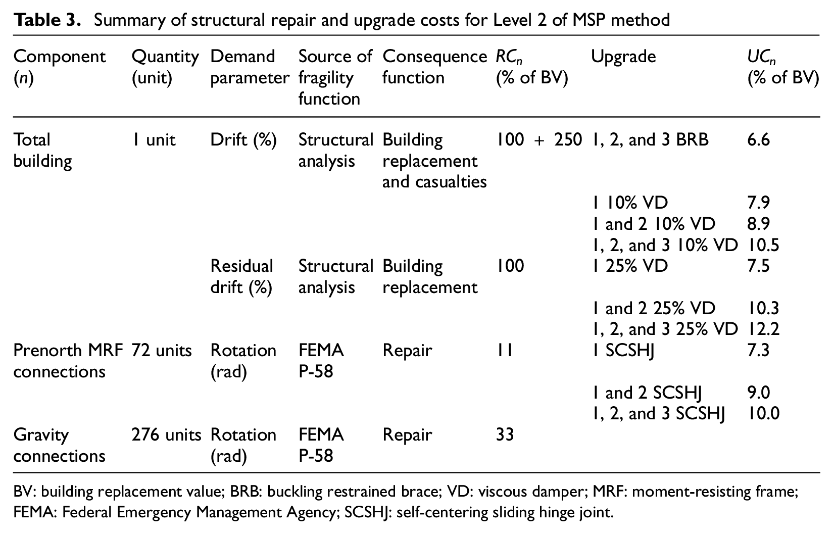
BV: building replacement value; BRB: buckling restrained brace; VD: viscous damper; MRF: moment-resisting frame; FEMA: Federal Emergency Management Agency; SCSHJ: self-centering sliding hinge joint.

Step 3: analysis of upgrade designs

The performance of each structural upgrade design was evaluated using the same multiple stripe analysis process used for the original structure but with updated first-mode periods when required. Table 4 summarizes the obtained Q_θ values for each structural upgrade design and also includes the values of Q_β to demonstrate the validity of approximating Q_β as 1.0 in the MSP method.

Table 4.

Calculated Q_θ values for Level 2 of MSP method

Upgrade design	CollapseQ_θ,C (Q_β)	Residual drift Q_θ,NR (Q_β)	Floor acceleration Q_θ,accel (Q_β)	Floor driftQ_θ,drift (Q_β)
BRB	1.45 (1.03)	1.31 (1.07)	1.45 (1.14)	0.41 (1.07)
1 SCSHJ	1.40 (0.81)	1.39 (0.88)	1.12 (1.02)	1.28 (1.03)
1 and 2 SCSHJ	1.30 (0.80)	1.34 (0.87)	1.20 (1.01)	1.29 (1.03)
1, 2, and 3 SCSHJ	1.51 (0.79)	1.54 (0.90)	1.25 (1.02)	1.31 (1.05)
1 10% VD	1.57 (0.93)	1.40 (1.03)	0.58 (1.00)	0.43 (1.03)
1 and 2 10% VD	1.68 (0.97)	1.56 (0.99)	0.51 (1.02)	0.25 (1.02)
1, 2, and 3 10% VD	1.85 (0.99)	1.64 (0.98)	0.45 (1.03)	0.21 (1.04)
1 25% VD	1.60 (0.92)	1.52 (0.97)	0.58 (0.99)	0.25 (1.05)
1 and 2 25% VD	1.78 (0.90)	1.73 (0.94)	0.52 (0.99)	0.19 (1.01)
1, 2, and 3 25% VD	2.39 (0.95)	1.96 (0.91)	0.43 (1.02)	0.16 (1.01)
Nonstructural only	1.00 (1.00)	1.00 (1.00)	1.00 (1.00)	1.00 (1.00)

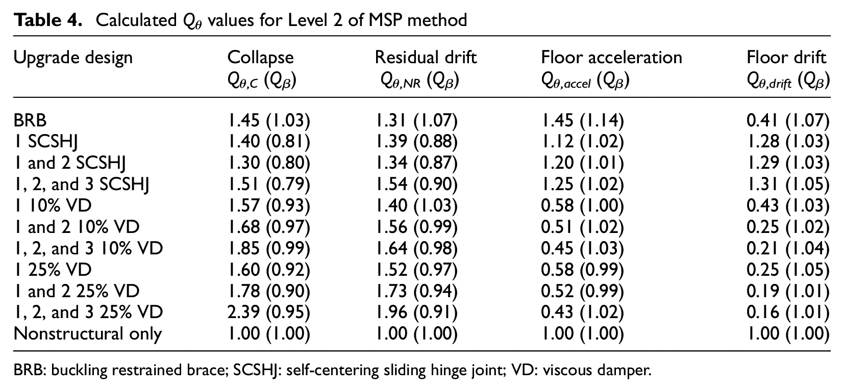
BRB: buckling restrained brace; SCSHJ: self-centering sliding hinge joint; VD: viscous damper.

EAL values for all four loss categories are shown in Figure 8 for all structural configurations in both scenarios (original and upgraded) as a function of their respective Q_θ values. A function correlating EAL to Q_θ values was fitted for each of the loss categories and shown in Figure 8. While the type of function is determined from the nature of the calculation of the annual frequency of occurrence of damage (λ(DS)), as described in the “Annual frequency of damage and mean annual loss” subsection, the regression constants of each function are unique to this case study. Furthermore, the cause for the imperfect correlation of the EAL(Q_θ) functions is the result of the small deviations in lognormal standard deviation from the original to the upgraded curves, as shown in Table 4. When considering only net benefit from the structural upgrade designs without the inclusion of the nonstructural options, the results shown in Figure 8 indicate that the various viscous damping designs are the only structural upgrades that lower the EAL in all four categories. While all structural upgrade designs provide reductions in losses caused by both collapse and non-reparable residual drifts by increasing the median value of both curves, the BRB and SCSHJ upgrades increase some of the floor hazard values resulting in increased EALs, as shown in Figure 8. The BRB upgrade increases the peak floor accelerations, causing the increase in EALs associated with the acceleration-sensitive nonstructural components to outweigh the total decreases in EAL from the other three loss categories, resulting in a net negative change in EAL due to structural changes alone.

Figure 8.

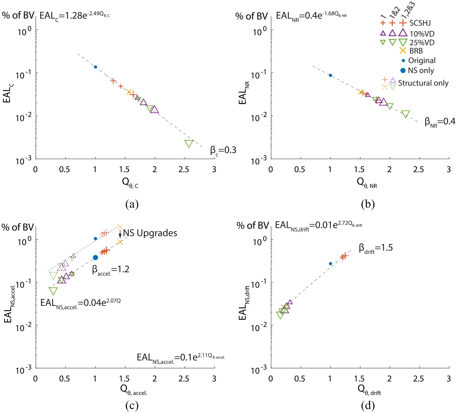
EAL values for all four loss categories.

Step 4: nonstructural upgrades

The selection of nonstructural components for upgrade was identical to Step 4 of Level 1, with the distinguishing feature of using the floor hazard curve calculated using the results of the multiple stripe analyses, as described in the “Hazards” subsection. For all upgrade designs, only acceleration-sensitive nonstructural component upgrades had BCR values exceeding one at this amortization value, as will be discussed in the Level 3 subsection. Since the BRB and SCSHJ structural upgrades induced the largest floor hazards, these structural upgrades led to the most extensive implementation of nonstructural upgrades as their larger values of f(EDP) increase the BCR value in Equation 19 for all nonstructural component upgrades. Since the results used in Figure 8 do not indicate the viability of each structural upgrade design, the changes in EAL values as well as the upgrade costs are summarized in Table 5 for each of the 10 structural upgrade designs. Each row shown in Table 5 is the result for that structural upgrade design at the specific amortization value, with each nonstructural upgrade being selected only when it provided a net positive benefit to the NPV for that particular structural upgrade strategy.

Table 5.

Summary of change in EAL for each structural upgrade and net positive nonstructural upgrade

Upgrade design	Storyimplementation	Δ(EAL_C)(% of BV)	Δ(EAL_NR)(% of BV)	Δ(EAL_accel.)(% of BV)	Δ(EAL_drift)(% of BV)	Δ(EAL_T)(% of BV)	Cost(% of BV)	BCR 2%/40years	NPV withnonstructuralupgrade (% of BV)r = 2%, t = 40 years	NPV without nonstructural upgrade(% of BV) r = 2%,t = 40 years
NS only	1, 2, and 3	0	0	0.67	0	0.67	6.43	2.85	11.90	0.0
SCSHJ	1	0.06	0.06	0.56	−0.11	0.57	13.64	1.14	1.95	−13.3
	1 and 2	0.05	0.05	0.52	−0.12	0.50	15.38	0.89	−1.70	−17.51
	1, 2, and 3	0.08	0.06	0.48	−0.14	0.48	16.60	0.79	−3.47	−19.96
BRB	1, 2, and 3	0.08	0.05	0.18	0.26	0.57	12.99	1.20	2.60	−21.97
10% VD	1	0.09	0.06	0.79	0.25	1.19	12.94	2.52	19.61	10.94
	1 and 2	0.09	0.06	0.87	0.26	1.28	13.85	2.53	21.17	14.43
	1, 2, and 3	0.10	0.07	0.90	0.26	1.33	15.46	2.35	20.92	14.90
25% VD	1	0.09	0.06	0.80	0.26	1.21	12.60	2.63	20.50	12.43
	1 and 2	0.10	0.07	0.87	0.27	1.31	15.28	2.35	20.56	13.43
	1, 2, and 3	0.11	0.08	0.89	0.27	1.35	15.01	2.46	21.92	17.39

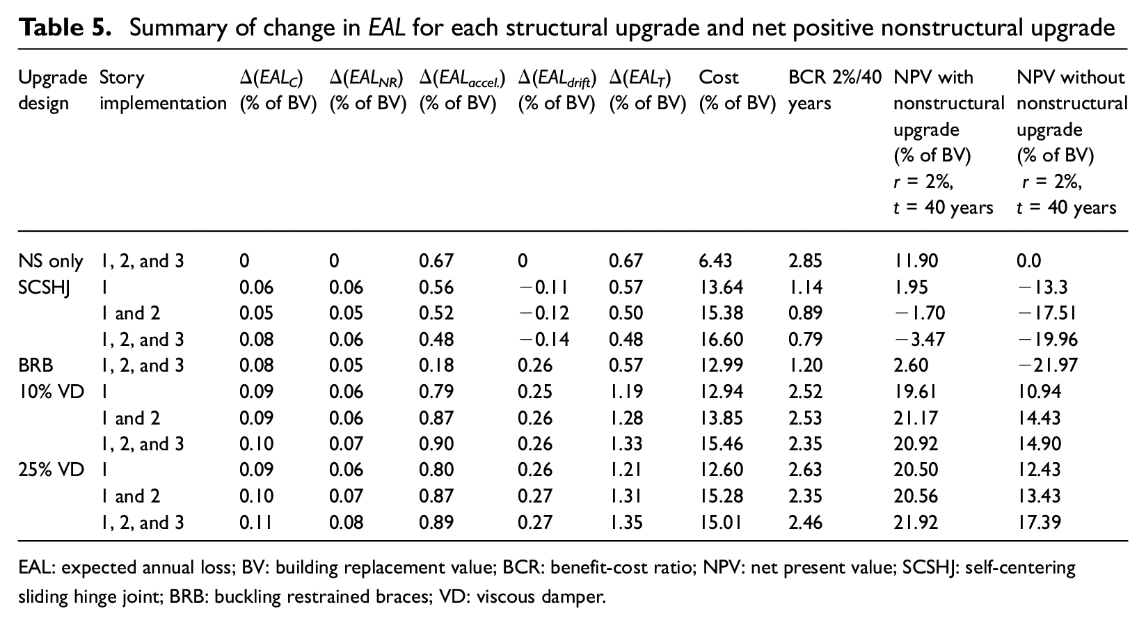
EAL: expected annual loss; BV: building replacement value; BCR: benefit-cost ratio; NPV: net present value; SCSHJ: self-centering sliding hinge joint; BRB: buckling restrained braces; VD: viscous damper.

Step 5: evaluation of NPV

The final step in the Level 2 analysis is the evaluation of the NPV of each upgrade design. This consists of the summation of all changes in EAL obtained from the previous step (Δ(EAL_T)), as well as the summation of all upgrade costs identified in Steps 2 and 4. Using these values, along with the amortization of the owner profile, the NPV was calculated using Equation 1 and is presented as a percentage of the building value. These values are shown in Table 5 for each upgrade design, along with an overall BCR value, which indicates the most efficient upgrade designs. To illustrate the effect of structural and nonstructural upgrades, the change in losses associated with each of the 11 designs (10 structural and 1 nonstructural only) was calculated with and without the inclusion of the nonstructural upgrades.

For this case study example, the upgrade design considering only nonstructural components has the highest BCR value of all upgrade designs, suggesting that this upgrade design is the most efficient. However, the NPV indicates that the largest net benefit is obtained when implementing the viscous damper upgrade with 25% damping in all three stories. The difference in which upgrade strategy seem most desirable according to the BCR versus the NPV indicates a diminishing return on investment when the BCR reduces but is still greater than 1.00. The NPV of the scenario considering only structural upgrades highlights the net negative result obtained when implementing the BRB and SCSHJ upgrades discussed earlier. The benefit of including nonstructural upgrades with each structural upgrade design is identified by comparing the two NPV value columns, where the MSP method identifies nonstructural upgrades with a net benefit of 11.9% when considering the original structure, 24.5% with the BRB upgrade, but only 4.5% for the 25% viscous damping upgrade at all stories because fewer nonstructural components are susceptible to the reduced demands in this case. However, including nonstructural component upgrades indicates that 9 of the 11 considered structural upgrade designs result in a positive NPV, so these could be included as options in a Level 3 analysis. The list of options to consider could be further shortened by considering only a subset of options that have the best expected NPV (i.e. viscously damped in this example) or are the most practical for the situation.

Potential modification to Step 4: iteration of BCR in MSP method

To improve the accuracy of a Level 2 analysis, an iterative BCR evaluation process was implemented in the Level 2 MSP method to account for the shared upgrade tasks across upgrades, as mentioned in the “Level 3: optimization using Monte Carlo PBEE evaluation” subsection. The addition of upgrade cost iterations to the MSP method, referred to as MSPIT, began from the initial BCR values previously obtained for each individual upgrade. The tasks required for all upgrades are then identified, and the upgrade cost of all components are reduced by removing duplications of the same tasks. The BCR values are then recalculated with the reduced costs. This iteration process is repeated until no new upgrades are identified. However, the shared consequence functions and costs reductions due to economies of scale, both of which are captured in the Level 3 analysis (see “Level 3: optimization using Monte Carlo PBEE evaluation” subsection), are still not reflected in this proposed MSPIT method.

Level 3: optimizing upgrades using genetic algorithm

The archetype structure and the maximization of the economic NPV in Equation 1 at the 2% rate of return and 40-year occupancy is identical to the archetype scenario presented by Steneker et al. (2020) and that study serves herein as the Level 3 analysis. The GA optimization run was repeated 100 times, and the rate at which components were selected in the optimal solution at each value was recorded. These are summarized in Figure 9 and range from values of 100 for components whose upgrade was selected in every analysis, to 0 for components whose upgrade was never selected. Figure 9 also lists the results obtained from the MSP method used in the Level 2 analysis and the modified MSPIT method presented in the “Potential modification to step: iteration of BCR in MSP method” subsection. All three approaches resulted in the selection of 25% viscous damping as the optimal structural upgrade design, and the identification of various nonstructural mechanical equipment for upgrade. However, while all three approaches have some similarities in component selection, the systemic differences caused by the factors presented in the “Level 3: optimization using Monte Carlo PBEE evaluation” subsection become apparent across the selected components. By taking advantage of the task sharing accounting, the GA and MSPIT identified several additional nonstructural component upgrades as optimal when compared to the MSP method, such as the piping systems that can be installed using common suspended trapeze restraint systems.

Figure 9.

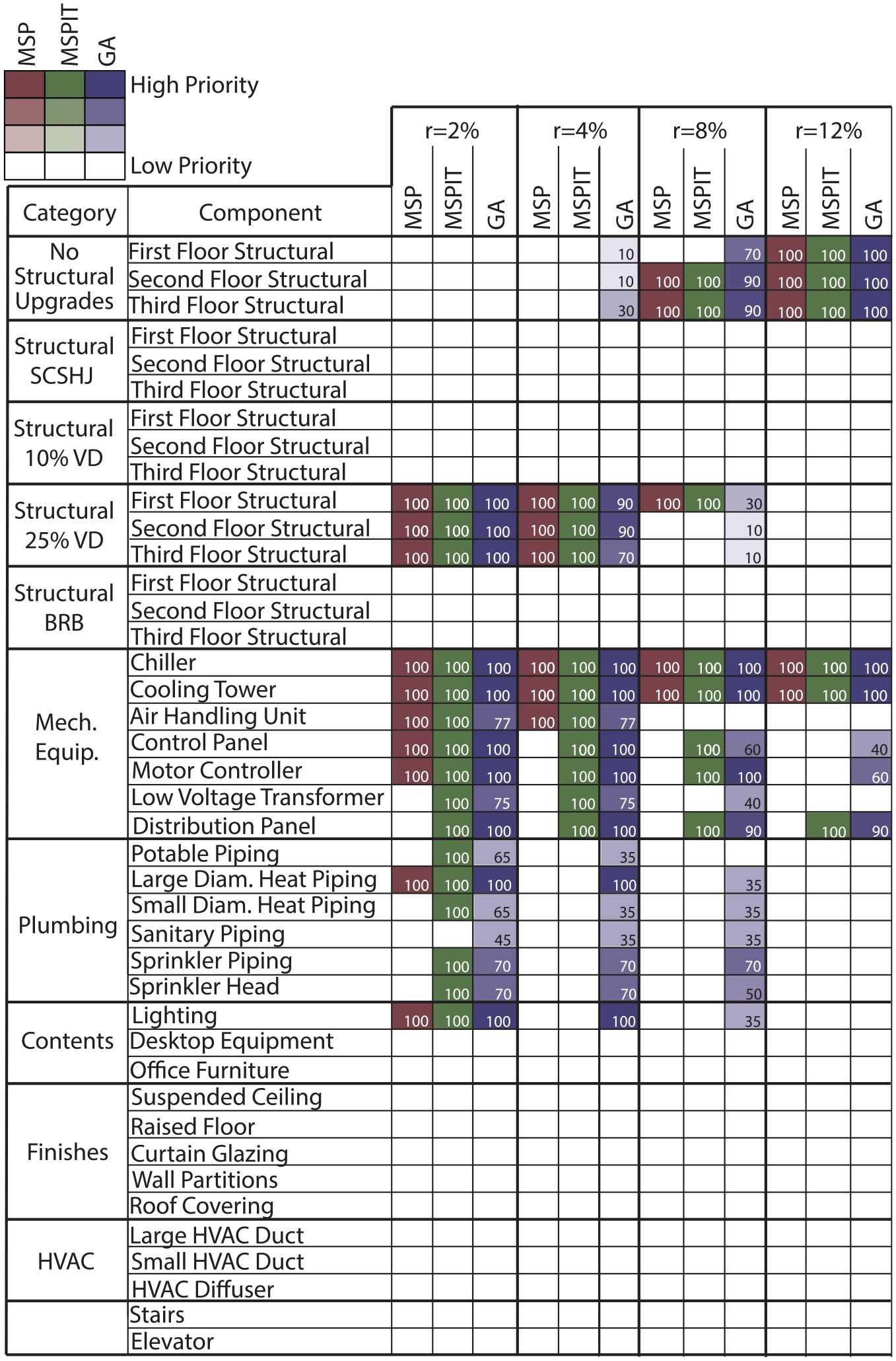
Comparison of selected upgrades (for occupancy time = 40 years).

Influence of rates of return

Figure 9 also includes the selection of components and designs for the optimal upgrade selected by the MSP, MSPIT, and GA methods at three other rates of return, representing increasing levels of risk accepted by the building owner, as mentioned in the study by Steneker et al. (2020). The differences in optimal selection between the MSP analysis and the GA analysis noted above for the 2% rate of return become more apparent at higher rates, where the BCR values obtained by Equation 19 reduces for all nonstructural components, leading to the de-prioritization of some in the GA and their non-selection in the MSP method. The MSPIT method identifies upgrades to the piping system at the lower rates of return but does not identify as many nonstructural components as candidates for upgrade as the GA at the higher rates.

Figure 10 summarizes the comparison between the MSP, MSPIT, and GA method by quantifying the total upgrade cost of the optimal solution obtained from all three methods at rates of return ranging from 2% to 16% with an occupancy time of 40 years. For the GA method, the upgrade costs are the mean value of the 100 solutions obtained at each rate. The results of each method are shown fitted with an exponential decay curve. The differences in identified optimal upgrade costs, visualized in Figure 10, show that the Level 3 GA method leads to the highest upgrade cost at all rates of return, followed by the MSPIT, which underestimates the optimal upgrade cost by 1% to 3% at all rates of return but mirrors the GA results in both scope and component upgrade selection. Finally, while the MSP curve identifies all of the upgrades with the largest benefit to cost ratio, it only captures approximately two-thirds of the total optimal solution obtained by the Level 3 GA method, missing potentially worthwhile upgrades that have a relatively small positive contribution to the upgrade NPV. This indicates that the MSP method is a viable tool for the Level 1 and Level 2 goals of assessing the viability of seismic upgrades, and can become more accurate with the addition of an iterative approach to determine upgrade costs. However, a Level 3 analysis using a scenario-based optimization approach, such as the GA, still provides further optimization refinement.

Figure 10.

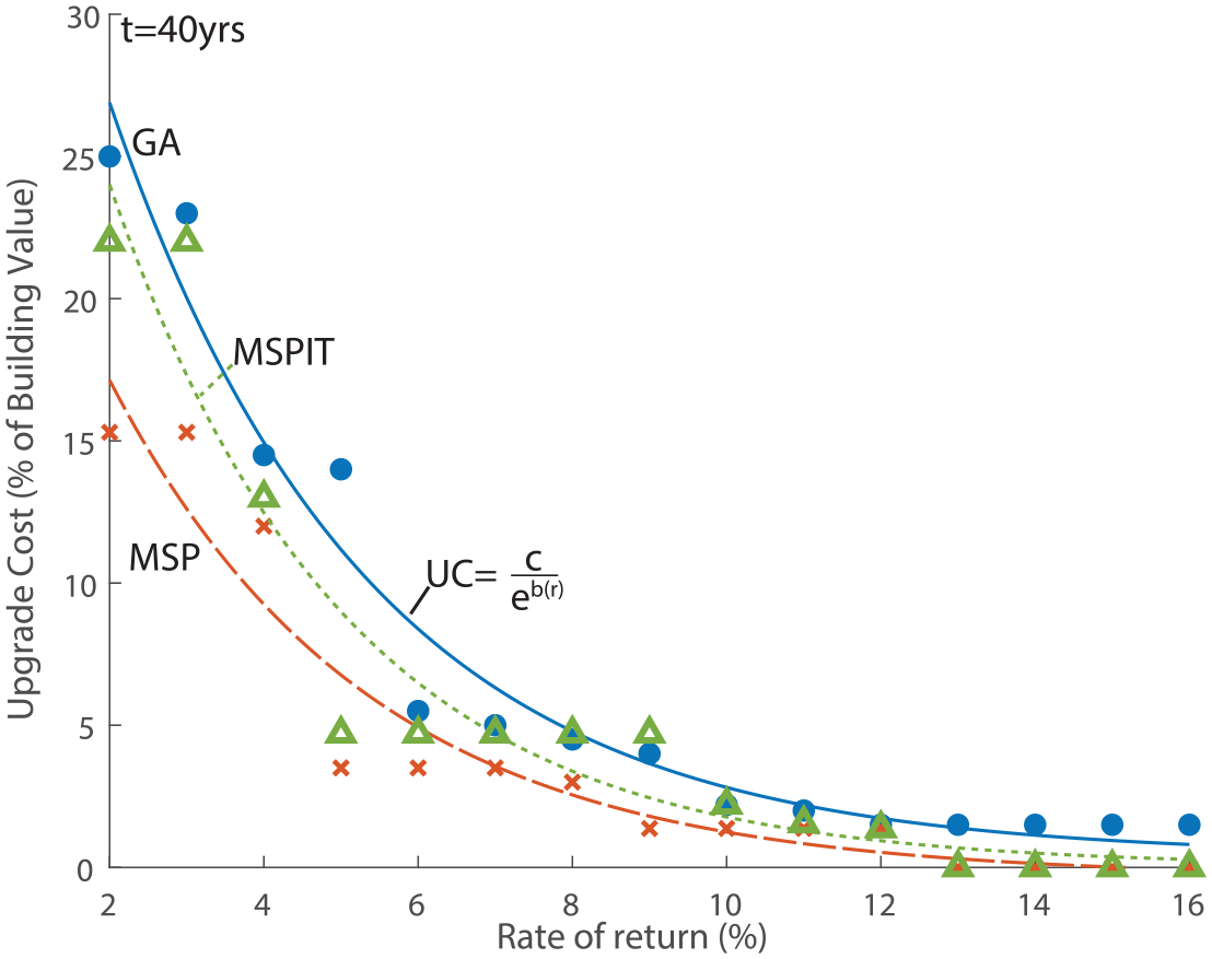
Total optimal upgrade cost obtained from each method.

Conclusion

This article provides a framework to identify and assess the viability of seismic upgrades considering both structural and nonstructural components options. The three-level framework is structured to initially require relatively low computational resources and provides quantifiable milestones to indicate the continued estimated viability of the seismic upgrades being considered. This provides a tiered workflow that encourages milestone conversations between the design professional and the client before further resources are committed. While the third level of the framework utilizes a previously developed GA optimization implementation structured around the Monte Carlo PBEE analysis, the initial two levels of the framework use the MSP method, a rapid PBEE implementation method introduced in this article. The MSP method measures the losses caused by different structural and nonstructural DSs while formalizing the relationships between structural and nonstructural component performance through the consideration of probability distributions, which define both structural performance and floor hazards. Each upgrade option is quantified by a shift in the median value of these curves. A case study example of the first two levels of the framework using a three-story steel MRF archetype structure led to an optimized solution for a upgrade strategy, which was then compared with results from a Level 3 analysis previously published by the authors. These observations indicate that the preliminary analysis provided by the use of the MSP method in the first two levels of the framework provided good indications of the optimal and viable upgrade strategy for a fraction of the computational effort required for the detailed Level 3 optimization.

As this framework provides a formal interpretation of the impact of structural modifications on the viability of seismic upgrades, continued research is required to provide guidance on the influence of various structural upgrades applied to different probability distributions of common archetype structures. The assumed shift in performance due to an upgrade (the Q_θ factors in Step 3 of the MSP process in Level 1) is a critical step in determining the viability of a structural upgrade, so developing guidance to more accurately estimate the behavior associated with an upgrade during preliminary design would allow for more certainty of a positive result before conducting Level 2 analysis. This would be possible if future studies of seismic structural upgrade approaches included quantification of structural response in terms of a shift in median probability distribution values (Q_θ). Furthermore, the required use of NLTHA for a Level 2 analysis can be considered cumbersome by practitioners. A method of obtaining floor EDP hazard curves with simplified analytical models, such as with the use of equivalent SDOF, could provide a viable alternative to this resource intensive process. Finally, future case studies would also provide examples from which empirical guidelines on future upgrade implementations can be determined. The final target use of this methodology is to encourage all stakeholders to invest in improving the seismic resiliency of buildings by identifying strategies having a net positive impact on the interest of all parties.

Footnotes

Declaration of conflicting interests

The author(s) declared no potential conflicts of interest with respect to the research, authorship, and/or publication of this article.

Funding

The author(s) received no financial support for the research, authorship, and/or publication of this article.

Supplemental material

Supplemental material for this article, including Appendix A, is available online.

ORCID iD

Lydell Wiebe

References

Almufti

Willford

(2013) Resilience-Based Earthquake Design Initiative (REDi^™) Rating System. London: Advanced Technology and Research (ARUP) Publications.

American Institute of Steel Construction (AISC) (2016) Specification for Structural Steel Buildings (ANSI/AISC 360-16). Chicago, IL: AISC.

American Society of Civil Engineers (ASCE) (2017) Seismic Evaluation and Retrofit of Existing Buildings (ASCE 41-17). Reston, VA: ASCE.

Arifin

Sullivan

MacRae

Kurata

Takeda

(2021) Lessons for loss assessment from the Canterbury earthquakes: A 22-storey building. Bulletin of Earthquake Engineering 19: 2081–2104.

Baker

(2015) Efficient analytical fragility function fitting using dynamic structural analysis. Earthquake Spectra 31(1): 579–599.

Baker

Lee

(2017) An improved algorithm for selecting ground motions to match a conditional spectrum. Journal of Earthquake Engineering 22(4): 708–723.

Behr

(1998) Seismic performance of architectural glass in mid-rise curtain wall. Journal of Architectural Engineering 4(3): 94–98.

Bianchi

Ciurlanti

Pampanin

(2021) Comparison of traditional vs low-damage structural and non-structural building systems through a cost/performance-based evaluation. Earthquake Spectra 37(1): 366–385.

Bradley

Dhakal

Cubrinovski

MacRae

Lee

(2009) Seismic loss estimation for efficient decision making. Bulletin of the New Zealand Society for Earthquake Engineering 42(2): 96–110.

10.

Bull

D. K.

(2011). “Stairs and Access Ramps between Floors in Multi-storey Buildings. A report o the Canterbury Earthquakes Royal Commission.”, Holmes Consulting Group, Christchurch, N.Z., 8.

11.

Cardone

Gesualdi

Perrone

(2019) Cost-benefit analysis of alternative retrofit strategies for RC frame buildings. Journal of Earthquake Engineering 23(2): 208–241.

12.

Chakravarti

Laha

Roy

(1967) Handbook of Methods of Applied Statistics, vol. 1. New York: John Wiley & Sons, pp. 392–394.

13.

Chopra

(2012) Dynamics of Structures. 4th ed. London: Pearson Education.

14.

Christopoulos

Filiatrault

(2006) Principles of Passive Supplemental Damping and Seismic Isolation. Pavia: IUSS Press.

15.

Comerio

(2000) The Economic Benefits of a Disaster Resistant University: Earthquake Loss Estimation for UC Berkeley. Berkeley, CA: Department of Architecture, University of California, Berkeley.

16.

Department of Homeland Security (DHS)/Federal Emergency Management Agency (FEMA) (2007) Multi-Hazard Loss Estimation Methodology: Earthquake Model, Hazus^®-MH MR3 Technical Manual. Washington, DC: National Institute of Building Sciences (NIBS), FEMA.

17.

Federal Emergency Management Agency (FEMA) (2000) Recommended seismic evaluation and upgrade criteria for existing welded steel moment-frame buildings. Report no. FEMA-351, June. Washington, DC: FEMA.

18.

Federal Emergency Management Agency (FEMA) (2009) Quantification of building seismic performance factors. Report no. FEMA P-695, June. Washington, DC: FEMA.

19.

Federal Emergency Management Agency (FEMA) (2012) Reducing the risks of nonstructural earthquake damage—A practical guide. Report no. FEMA E-74, January. Washington, DC: FEMA.

20.

Federal Emergency Management Agency (FEMA) (2018) Seismic performance assessment of buildings—Methodology. Report no. FEMA P-58, August. Washington, DC: FEMA.

21.

Filiatrault

Kuan

Tremblay

(2004) Shake table testing of bookcase—Partition wall systems. Canadian Journal of Civil Engineering 31: 664–676.

22.

Flores

Lopez-Garcia

Charney

(2015) Floor accelerations in buildings having different structural systems. In: Proceedings of the ASCE structures congress, Portland, OR, 23–25 April.

23.

Galanis

Sycheva

Mimra

Stojadinovic

(2018) A framework to evaluate the benefit of seismic upgrading. Earthquake Spectra 34: 527–548.

24.

Günay

Mosalam

(2013) PEER performance-based earthquake engineering methodology, revisited. Journal of Earthquake Engineering 17(6): 829–858.

25.

Gupta

Krawinkler

(1999) Seismic demands for performance evaluation of steel moment resisting frame buildings. Report no. 132, June. Stanford, CA: Department of Civil and Environmental Engineering, Stanford University.

26.

Hofer

Zanini

Faleschini

Pellegrino

(2018) Profitability analysis for assessing the optimal seismic retrofit strategy of industrial productive processes with business-interruption consequences. Journal of Structural Engineering: ASCE 144(2): 04017205.

27.

Ibarra

Medina

Krawinkler

(2005) Hysteretic models that incorporate strength and stiffness deterioration. Earthquake Engineering & Structural Dynamics 34: 1489–1511.

28.

Khoo

H-H

Clifton

Butterworth

MacRae

Gledhill

Sidwell

(2012) Development of the self-centering Sliding Hinge Joint with friction ring springs. Journal of Constructional Steel Research 78: 201–211.

29.

Liel

Haselton

Deierlein

Baker

(2009) Incorporating modeling uncertainties in the assessment of seismic collapse risk of buildings. Structural Safety 31: 197–211.

30.

Lucchini

Franchin

Mollaioli

(2017) Uniform hazard floor response spectra for linear structures. Earthquake Engineering & Structural Dynamics 46(7): 1121–1140.

31.

McKenna

Fenves

Scott

(2000) Open System for Earthquake Engineering Simulation. Berkeley, CA: University of California, Berkeley.

32.

Mayes

Wetzel

Weaver

Tam

Parker

Brown

Pietra

(2013) Performance based design of buildings to assess damage and downtime and implement a rating system. Bulletin of the New Zealand Society for Earthquake Engineering 46(1): 40–55.

33.

Merino

Perrone

Filiatrault

(2019) Consistent floor response spectra for performance-based seismic design of nonstructural elements. Earthquake Engineering & Structural Dynamics 49(3): 261–284.

34.

Miranda

Aslani

(2003) Probabilistic response assessment for building-specific loss estimation. PEER report no. 2003/03, September. Berkeley, CA: Pacific Earthquake Engineering Research (PEER) Center, University of California, Berkeley.

35.

Miranda

Taghavi

(2003) Estimation of seismic demands on acceleration-sensitive nonstructural components in critical facilities. ATC-29-2 report, 23–24 October. Redwood City, CA: Applied Technology Council (ATC).

36.

Moon

K-H

Han

Lee

Seok

(2012) Approximate MPA-based method for performing incremental dynamic analysis. Nonlinear Dynamics 67: 2865–2888.

37.

O’Reilly

Calvi

(2020) Quantifying seismic risk in structures via simplified demand–Intensity models. Bulletin of Earthquake Engineering 18: 2003–2022.

38.

O’Reilly

Monteiro

(2019) Probabilistic models for structures with bilinear demand-intensity relationships. Earthquake Engineering & Structural Dynamics 48(2): 253–268.

39.

PEER (2013) PEER NGA-West2 Database. PEER Report No. 2013/03, May. Pacific Earthquake Engineering Research Center, Berkeley, CA, USA

40.

Perrone

Cardone

O’Reilly

Sullivan

(2019) Developing a direct approach for estimating expected annual losses of Italian buildings. Journal of Earthquake Engineering. Epub ahead of print 19 September. DOI: 10.1080/13632469.2019.1657988.

41.

Retamales

Davies

Mosqueda

Filiatrault

(2013) Experimental seismic fragility of cold-formed steel framed gypsum partition walls. Journal of Structural Engineering: ASCE 139(8): 1285–1293.

42.

RSMeans (2018) Commercial Renovation Cost Data. Norwell, MA: Reed Construction Data.

43.

Shilling

Wurtzebach

(2012) Is value-added and opportunistic real estate investing beneficial? If so, why? Journal of Real Estate Research 34(4): 429–461.

44.

Soroushian

Zaghi

Maragakis

Echevarria

Tian

Filiatrault

(2015) Analytical seismic fragility analyses of fire sprinkler piping systems with threaded joints. Earthquake Spectra 31(2): 1125–1155.

45.

Steneker

(2020) Towards more optimized and resilient seismic design of buildings with steel moment resisting frames. PhD Thesis, McMaster University, Hamilton, ON, Canada.

46.

Steneker

Filiatrault

Wiebe

Konstantinidis

(2020) Integrated structural-nonstructural performance-based seismic design and retrofit optimization of buildings. Journal of Structural Engineering: ASCE 146: 04020248.

47.

Steneker

Wiebe

Filiatrault

(2021) Seismic response comparison of steel MRFs with yielding and low-damage connections. Journal of Constructional Steel Research 179: 106502.

48.

Sullivan

Calvi

Nascimbene

(2013) Towards improved floor spectra estimates for seismic design. Earthquakes and Structures 4(1): 109–132.

49.

Sullivan

Welch

Calvi

(2014) Simplified seismic performance assessment and implications for seismic design. Earthquake Engineering and Engineering Vibration 13: 95–122.

50.

Uniform Building Code (UBC) (1994) Structural Engineering Design Provisions, vol. 2. Lansing, MI: International Conference of Building Officials (ICBO).

51.

United States Department of Transportation (DOT) (2016) Guidance on Treatment of the Economic Value of a Statistical Life (VSL) in US Department of Transportation Analyses – 2016 Adjustment. Washington, DC: DOT.

52.

United States Geological Survey (USGS) (2014) Unified Hazard Tool (version 4.1.9, Lat: 47.6, Long: -122.3, T: 1.0 Sec). Reston, VA: USGS.

53.

Welch

Sullivan

Calvi

(2014) Developing direct displacement-based procedures for simplified loss assessment in performance-based earthquake engineering. Journal of Earthquake Engineering 18: 290–322.

54.

Yeow

Orumiyehei

Sullivan

MacRae

Clifton

Elwood

(2018) Seismic performance of steel friction connections considering direct-repair costs. Bulletin of Earthquake Engineering 16: 5963–5993.

A framework for the rapid assessment of seismic upgrade viability using performance-based earthquake engineering

Abstract

Keywords

Introduction

Overview of proposed framework

Key parameters of MSP method

Performance of structures and nonstructural components

Site hazards and floor hazards

Annual frequency of damage and mean annual loss

Deaggregation of change in loss by hazard intensity

Deaggregation of the influence of upgrades on losses

Influence of changes to the collapse fragility of the structure

Influence of changes to non-reparable residual drift fragility of the structure

Influence of changes to the floor hazard

Influence of changes to the fragility of nonstructural components

Discussion of framework levels

Level 1: MSP method for feasibility study of upgrade strategy

Level 2: MSP method for verification of schematic design of upgrade strategy

Level 3: optimization using Monte Carlo PBEE evaluation

Case study example

Level 1 analysis

Step 1: original conditions

Step 2: upgrade cost and structural behavior

Steps 3 and 4: required change in EAL and approximation of Qθ values

Step 5: determination of attainability of Qθ values

Level 2 analysis

Step 1: original conditions

Step 2: upgrade design, cost, and performance

Step 3: analysis of upgrade designs

Step 4: nonstructural upgrades

Step 5: evaluation of NPV

Potential modification to Step 4: iteration of BCR in MSP method

Level 3: optimizing upgrades using genetic algorithm

Influence of rates of return

Conclusion

Footnotes

Declaration of conflicting interests

Funding

Supplemental material

ORCID iD

References

Steps 3 and 4: required change in EAL and approximation of Q_θ values

Step 5: determination of attainability of Q_θ values