Sage Journals: Discover world-class research

Abstract

Propositional logic (as other logics) can be seen as a way to represent sets of states of the world (by the sets of models of formulas). Representation of variations from a set of states of the world to another is motivated by studies on case-based reasoning (CBR): the comparison of two problems and the way a solution is transformed into another solution can be seen as variations from a set of states to another. This has led to a notation for representing these variations (a syntax) and this article studies how to associate to this notation a semantics based on model theory in which an interpretation is an ordered pair of interpretations in propositional logic. The article presents a classical study of this logic (syntax, semantics, properties, a formal system, etc.). It also explains how CBR can benefit from this logic, in particular through the representation of adaptation rules and to a case-based inference algorithm using such rules.

Keywords

knowledge representation representing variations case-based reasoning adaptation rules

1. Introduction

Case-based reasoning (CBR; Riesbeck & Schank, 1989) is a reasoning based on a case base $CB$ where a case is, in general, given by an ordered pair $(x, y)$ where $x$ represents a problem (of the application domain under consideration) and $y$ represents a solution to this problem. A CBR session takes as input a problem $x^{tgt}$ to be solved (the target problem) and consists usually of two reasoning steps: retrieval and adaptation. Retrieval consists in selecting a case $(x^{s}, y^{s}) \in CB$ such that $x^{s}$ is deemed similar to $x^{tgt}$ . Adaptation consists in modifying $y^{s}$ with the aim of solving the target problem. A principle often used for adaptation is based on the intuitive notion of variations between problems and between solutions:

(1)
Computation of the variation from $x^{s}$ to $x^{tgt}$ , denoted by $Δ x$ ;
(2)
Computation of $Δ y$ , the variation from $y^{s}$ to the solution to be found, on the basis of $Δ x$ ;
(3)
Computation of $y^{tgt}$ , from $y^{s}$ and $Δ y$ , where $y^{tgt}$ is a plausible solution to $x^{tgt}$ . Note that, in general, CBR is a hypothetical reasoning: the solution it provides solves plausibly the target problem.

Step (2) above is typically based on adaptation knowledge which is often represented by adaptation rules. In general, the premises of such a rule contain the variation between problems and, its conclusion, a variation between solutions: “If two problems change according to $Δ x$ then their solutions change according to $Δ y$ .” Such rules can be learned from the case base, according to a principle introduced in Hanney and Keane (1996) and that is sometimes called the case difference heuristics (e.g., in Leake et al., 2021). The idea is to apply a learning process using as learning set the ordered pairs $(Δ x^{i j}, Δ y^{i j})$ where $(x^{i}, y^{i}), (x^{j}, y^{j}) \in CB$ and $Δ x^{i j}$ (resp., $Δ y^{i j}$ ) is the variation from $x^{i}$ to $x^{j}$ (resp., from $y^{i}$ to $y^{j}$ ).

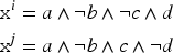
In some applications of CBR, problems and solutions can be represented by Boolean properties (or translated into this representation), that can be coded as conjunction of literals in propositional logic. For example, let us consider the two following problems:
$\begin{aligned} x^{i} & = a \land \neg b \land \neg c \land d \\ x^{j} & = a \land \neg b \land c \land \neg d \end{aligned}$
The variation from $x^{i}$ to $x^{j}$ has been noted in the following way in some studies on adaptation knowledge learning using the case difference heuristics:
$Δ x^{i j} = a^{= 1} \land b^{= 0} \land c^{+} \land d^{-}$
where $x^{v}$ means that the Boolean property $x$ varies according to $v$ , where $v = = 1$ (resp. $v = = 0$ ) means “stays true (resp. false)” and $v = +$ (resp. $v = -$ ) means “change from false to true (resp. from true to false).”

For instance, adaptation knowledge learning has been studied for $Taaable$ , a CBR system in the cooking domain (Cordier et al., 2014). Suppose that, in a recipe book (constituting a case base), ordered pairs $(c^{i}, c^{j})$ of dessert recipes can be found such that, $c^{i}$ has apple and cinnamon as ingredients and $c^{j}$ has pear and chocolate (but no pear and chocolate in $c^{i}$ and no apple and cinnamon in $c^{j}$ ). From these ordered pairs, the following adaptation rule can be learned:
In recipes of desserts with apples and cinnamon, these ingredients can be replaced by pears and chocolate.

This adaptation rule can be written by the following expression:
$AR = {rDessert}^{= 1} \land {iApple}^{-} \land {iCinnamon}^{-} \land {iPear}^{+} \land {iChocolate}^{+}$
(1)
(where $rDessert$ is the property to be a recipe of dessert, $iApple$ , the property to be a recipe with apple as ingredient, etc.)

The expressions such as the one presented above were only used as notations: the syntax was defined but not the semantics that would enable to draw inferences. The first objective of this article is to define this semantics and to study its properties. Starting from finite propositional logic $(L P, ⊨)$ , the logic $(Δ L P, ⊨)$ is defined, such that its syntax contains formulas such as the one introduced above and semantics is defined in a model-theoretic way. Then this logic is studied according to various aspects. The second objective is to study some benefits of using this logic for CBR, beyond the mere notation from which it originates.

The article is organized as follows. After some preliminaries (Section 2), the logic $(Δ L P, ⊨)$ is presented: its syntax, its semantics, and some general results related to it (Section 3). In Section 4, a formal system for this logic is presented, which is proven to be sound and complete. Section 5 deals with algorithmic aspects of this logic. This work originates from a notation used in CBR and Section 6 details two important issues of CBR through this logic: the representation of adaptation rules and a novel algorithm for CBR, including an efficient case retrieval step that is exact with respect to adaptation. Section 7 discusses some related works and Section 8 concludes the article and presents some future work. For some results, the proofs are given in Appendix Section A, in order to improve the readability of the article.
2. Preliminaries

These preliminaries are about propositional logic (Section 2.1) and CBR (Section 2.2).

2.1. Propositional Logic

$(L P, ⊨)$ is the basic logic on which $(Δ L P, ⊨)$ will be defined.

Let $V$ be a finite set of symbols; an element of $V$ is called propositional variable (or simply variable). A formula of $(L P, ⊨)$ is either a propositional variable or has one of the following forms: $\neg β$ , $β_{1} \land β_{2}$ , and $β_{1} \lor β_{2}$ , where $β$ , $β_{1}$ , and $β_{2}$ are propositional formulas. The following abbreviations are used ( $\underline{i a a f}$ is read “is an abbreviation for”):

⊤ \underline{i a a f} a \lor \neg a ⊥ \underline{i a a f} a \land \neg a β_{1} \to β_{2} \underline{i a a f} \neg β_{1} \lor β_{2} with an arbitrary variable a and β_{1}, β_{2} \in L P

A literal of

(L P, ⊨)

is a formula

a

\neg a

(for an

a \in V

). A cube in this logic is a conjunction of literals where every variable occurs at most once. A cube is complete if every variable occurs in it. The set of variables occurring in

α \in L P

is denoted by

V (α)

The semantics in model theory is defined as follows. An interpretation in propositional logic is a mapping $I : V \to {0, 1}$ , where ${0, 1}$ is the set of Booleans ( $0$ stands for false and $1$ stands for true). Let $Ω$ be the set of interpretations. Let $I \in Ω$ and $α \in L P$ . The relation “ $I$ satisfies $α$ ” (also read “ $I$ is a model of $α$ ” and denoted by $I ⊨ α$ ) is defined recursively as follows:

$I ⊨ a$ if $I (a) = 1$ for a variable $a$ ;

$I ⊨ \neg α$ if $I ⊭ α$ for an $α \in L P$ ;

$I ⊨ α_{1} \land α_{2}$ if $I ⊨ α_{1}$ and $I ⊨ α_{2}$ for $α_{1}, α_{2} \in L P$ ;

$I ⊨ α_{1} \lor α_{2}$ if $I ⊨ α_{1}$ or $I ⊨ α_{2}$ for $α_{1}, α_{2} \in L P$ .

The set of models of $α$ is written $M (α)$ . If $B$ is a finite set of formulas, $M (B)$ is the intersection of the $M (α)$ for $α \in B$ , which allows to assimilate $B$ to the conjunction $⋀ B$ of its elements. The relation $B$ entails $β$ ( $B ⊨ β$ ) is defined by $M (B) \subseteq M (β)$ , and the relation $α ⊨_{B} β$ is defined by $B \cup {α} ⊨ β$ . A formula $α$ is satisfiable when $M (α) \neq \emptyset$ (which is equivalent to $α ⊭ ⊥$ ). A formula $α$ is a tautology (denoted by $⊨ α$ ) if $M (α) = Ω$ . Finally, with $α, β \in L P$ , $α \equiv β$ if $M (α) = M (β)$ .

2.2. Case-Based Reasoning

Generalities. CBR is a type of reasoning relying on a case base, where a case is a representation of a problem solving episode. An application domain for CBR is given by a triplet $(P, S, ⇝)$ where $P$ and $S$ are sets and $⇝$ is a binary relation on $P \times S$ . An element $x \in P$ is called a problem, an element $y \in S$ , a solution, and $x ⇝ y$ is read “ $x$ has for solution $y$ ” or “ $y$ solves $x$ .”

In general, the relation $⇝$ is not completely known by the CBR system: the objective of the latter is to build a hypothesis of solution $y^{tgt}$ to a given problem, the target problem, denoted by $x^{tgt}$ .

It is often assumed (in particular, in this article) that a case is given by an ordered pair $(x, y) \in P \times S$ where $x ⇝ y$ : the relation $⇝$ is only known for a finite set that constitutes the case base. An element of the case base is denoted by $(x^{s}, y^{s})$ and is called a source case ( $x^{s}$ is the source problem).

The most common process of CBR consists in a retrieval step (selection of $k$ elements of the case base deemed similar to the target problem) and an adaptation step (reuse of the retrieved cases for solving $x^{tgt}$ ). In this article, only single case retrieval and single case adaptation are considered, that is, $k = 1$ . This means in particular that an adaptation problem is given by a source case and a target problem: it is noted $((x^{s}, y^{s}), x^{tgt})$ in the following.

Two ways of considering adaptation exist, that are inspired by the difference between transformational analogy and derivational analogy, two notions introduced by J. G. Carbonell (see Carbonell, 1983, 1986):

Transformational adaptation aims at solving the adaptation problem by reading it under the form “The solution searched for, $y^{tgt}$ , is to $y^{s}$ as $x^{tgt}$ is to $x^{s}$ .” It can be interpreted as follows: from variations between $x^{s}$ and $x^{tgt}$ , denoted by $Δ x$ , the variation between the solution $y^{s}$ and the unknown $y^{tgt}$ , denoted by $Δ y$ , is inferred, then, $y^{tgt}$ is inferred from $y^{s}$ and $Δ y$ .

Generative adaptation aims at solving the adaptation problem by reading it under the form “The solution searched for, $y^{tgt}$ , is to $x^{tgt}$ as $y^{s}$ is to $x^{s}$ .” It relies on the highlighting of the links between $x^{s}$ and $y^{s}$ and on the “replay” of this link on $x^{tgt}$ .

This article focuses on transformational adaptation: the study of the application of $(Δ L P, ⊨)$ to generative adaptation constitutes a potential future work.

CBR Knowledge Model. Usually, it is considered that the knowledge base of a CBR system is composed of four knowledge containers: the case base $CB$ , the domain knowledge $DK$ , the retrieval knowledge $RK$ , and the adaptation knowledge $AK$ (Richter & Weber, 2013). $CB$ and $AK$ have been mentioned above. $RK$ is often represented by a similarity measure or a distance function between problems. $DK$ can be considered as a conjunction of integrity constraints, where each of these constraints gives a necessary condition for a case to be licit. The inferences in the case representation formalism are usually made according to the domain knowledge: the relation $⊨_{DK}$ is used instead of simply $⊨$ .

Representing Cases in Propositional Logic. In some applications, cases can be represented in $(L P, ⊨)$ : the set $V$ is partitioned into ${V_{P}, V_{S}}$ and a problem $x$ (resp. a solution $y$ ) is represented by a formula whose variables belong to $V_{P}$ (resp. to $V_{S}$ ). A source case $(x^{s}, y^{s})$ is represented by the conjunction $x^{s} \land y^{s}$ . Sometimes, as it will be seen in the running example of Section 6, the partitioning in problem variables and solution variables is only done once the adaptation problem is specified: knowing $x^{tgt}$ and the source case $c^{s}$ , $V_{P}$ and $V_{S}$ are determined and then, $c^{s}$ can be written $x^{s} \land y^{s}$ .

In many applications, the source cases and the target problem are considered as specific, that is, coming from a particular experience and thus completely instantiated. In this situation, for a source case $(x^{s}, y^{s})$ and a target problem $x^{tgt}$ , the problems $x^{s}$ and $x^{tgt}$ can be written under the form $\underset{a \in V_{P}}{⋀} ℓ (a)$ and the solution $y^{s}$ under the form $\underset{a \in V_{S}}{⋀} ℓ (a)$ , where $ℓ (a) \in {a, \neg a}$ . Then, the formula $x^{s} \land y^{s}$ is a complete cube so $| M (x^{s} \land y^{s}) | = 1$ .

Adaptation Knowledge Learning. Adaptation is often based on adaptation knowledge. This knowledge can be acquired from experts (see, e.g., d’Aquin et al., 2006). It can also be learned from the case base, according to the principle called “difference heuristics” in Jalali et al. (2017) and initially defined in Hanney and Keane (1996). This principle relies on the principle of transformational adaptation: given two different source cases $(x^{i}, y^{i})$ and $(x^{j}, y^{j})$ , the variations $Δ x^{i j}$ , from $x^{i}$ to $x^{j}$ , and $Δ y^{i j}$ , from $y^{i}$ to $y^{j}$ , are built. Adaptation knowledge learning uses a set of ordered pairs $(Δ x^{i j}, Δ y^{i j})$ to produce a model of a mapping $Δ x \mapsto Δ y$ , which makes it possible, from a problem variation to obtain a solution variation, which is useful during a transformational adaptation process.

Some work in this framework has used the notation $a^{v}$ , where $a$ is a problem or solution attribute and where $v$ represents a relation between values of the domain of this attribute. Then, this notation makes it possible to encode these variations, for the purpose of adaptation rule learning using techniques such as closed itemset extraction (see d’Aquin et al., 2007, for a description of such a process). For example ${age}^{add (5)}$ indicates a variation of $+ 5$ for the attribute $age$ . The result of a frequent closed itemset extraction is a set of itemsets, an itemset in this adaptation rule learning process being a set of expressions $a^{v}$ . Considering only Boolean attributes, these $a^{v}$ are formulas of the logic $(Δ L P, ⊨)$ , which motivates the study of this logic.

3. The Logic of Propositional Variations

This section presents the logic $(Δ L P, ⊨)$ : its syntax (Section 3.1), its semantics (Section 3.2), some general results associated with it (Section 3.3), and two operators on this logic (Section 3.4).

3.1. Syntax of $(Δ L P, ⊨)$

A formula $φ \in Δ L P$ is an expression of one of the following forms: $α ▹ β$ (that can be read “ $α$ becomes $β$ ”), $\neg ψ$ , $ψ_{1} \land ψ_{2}$ and $ψ_{1} \lor ψ_{2}$ , where $α, β \in L P$ and $ψ, ψ_{1}, ψ_{2} \in Δ L P$ . The following abbreviations are used: When the context is not ambiguous, $⊤_{Δ}$ and $⊥_{Δ}$ are simply noted $⊤$ and $⊥$ . Let $D_{0} = {= 1, = 0, +, -}$ ; the elements of $D_{0}$ are called primitive variation symbols. The set $D_{1} = {=, \neq \neq, 0 ∙, 1 ∙, ∙ 0, ∙ 1}$ is the set of non primitive variation symbols. $D = D_{0} \cup D_{1}$ is therefore the set of variation symbols.

A literal of $(Δ L P, ⊨)$ is a formula of the form $a^{v}$ where $a \in V$ and $v \in D$ . A cube of this logic is a conjunction of literals in which any variable appears at most once. A cube is said primitive if every variation symbol occurring in it is primitive. A cube is complete if it is primitive and if every variable occurs in the cube.

For $φ \in Δ L P$ , $x \in V$ and $α \in L P$ , $φ [x ∖ α]$ is the result of the substitution of $x$ with $α$ in $φ$ defined in the usual way. The set of variables occurring in $φ$ is denoted by $V (φ)$ . The size of $φ$ , noted $| φ |$ , is the number of occurrences of connectives of $φ$ . A knowledge base of $(Δ L P, ⊨)$ is a finite subset of $Δ L P$ .

3.2. Semantics of $(Δ L P, ⊨)$

Two definitions of the semantics are given below: one with interpretations based on propositional logic interpretations and an alternative one based on the primitive symbols of variation. They define the same entailment relation. The former will be used more often, the latter is used mainly in some proofs.

3.2.1. A First Definition of Entailment

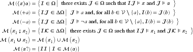
Let $Δ Ω = Ω \times Ω$ . An element $(I, J)$ of $Δ Ω$ is called interpretation (for this logic) and is simply written $I J$ . For $φ \in Δ L P$ , $I J ⊨ φ$ is defined as follows (where $α, β \in L P$ , $ψ, ψ_{1}, ψ_{2} \in Δ L P$ ):

$I J ⊨ α ▹ β$ if $I ⊨ α$ and $J ⊨ β$ .

$I J ⊨ \neg ψ$ if $I J ⊭ ψ$ .

$I J ⊨ ψ_{1} \land ψ_{2}$ if $I J ⊨ ψ_{1}$ and $I J ⊨ ψ_{2}$ .

$I J ⊨ ψ_{1} \lor ψ_{2}$ if $I J ⊨ ψ_{1}$ or $I J ⊨ ψ_{2}$ .

The set of models of

φ

is denoted by

M (φ) = {I J \in Δ Ω | I J ⊨ φ}

. It can be noted that

M (α ▹ β) = M (α) \times M (β)

. The notions of satisfiability, logical entailment (

⊨

), tautology, and logical equivalence (

\equiv

) are defined in the same way as in propositional logics.

3.2.2. An Alternative Definition of Entailment

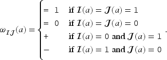
The relation $⊨$ between a knowledge base $B$ and a formula $φ$ of propositional variation logic can be redefined using four “truth values” given by the elements of $D_{0} = {= 1, = 0, +, -}$ .

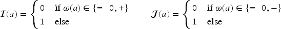
Let ${Δ Ω}_{alt}$ be the set of functions $ω : V \to D_{0}$ . Let $⊨_{alt}$ be the relation between an $ω \in {Δ Ω}_{alt}$ and a $φ \in Δ L P$ defined by:

ω ⊨_{alt} φ if \underset{a \in V}{⋀} a^{ω (a)} ⊨ φ

(2)

Let

M_{alt} (φ) = {ω \in {Δ Ω}_{alt} | ω ⊨_{alt} φ}

. For example, if

V = {a, b}

M_{alt} (a^{=} \land b^{+}) = {ω_{1}, ω_{2}}

where

ω_{1} (a) = = 1

ω_{2} (a) = = 0

, and

ω_{1} (b) = ω_{2} (b) = +

. For a knowledge base

B

, let

M_{alt} (B) = ⋂_{φ \in B} M_{alt} (φ)

. Then, the relation

⊨_{alt}

between a knowledge base

B

and a formula

φ

is defined by

B ⊨_{alt} φ

M_{alt} (B) \subseteq M_{alt} (φ)

This relation $⊨_{alt}$ does not define a new semantics of the logic of variations as the proposition below show; it only gives an alternative definition of this semantics.

Proposition 1

For every knowledge base $B$ of $(Δ L P, ⊨)$ and every $φ \in Δ L P$ , $B ⊨_{alt} φ$ iff $B ⊨ φ$ .

Proof.

Given $I J \in Δ Ω$ , let $ω_{I J} \in {Δ Ω}_{alt}$ be such that, for $a \in V$ ,

ω_{I J} (a) = {\begin{cases} = 1 & if I (a) = J (a) = 1 \\ = 0 & if I (a) = J (a) = 0 \\ + & if I (a) = 0 and J (a) = 1 \\ - & if I (a) = 1 and J (a) = 0 \end{cases} .

The function

I J \in Δ Ω \mapsto ω_{I J} \in {Δ Ω}_{alt}

is bijective and its inverse function is defined as follows. To

ω \in {Δ Ω}_{alt}

, it maps

I J \in Δ Ω

such that, for

a \in V

\begin{aligned} I (a) & = {\begin{cases} 0 & if ω (a) \in {= 0, +} \\ 1 & else \end{cases} J (a) = {\begin{cases} 0 & if ω (a) \in {= 0, -} \\ 1 & else \end{cases} \end{aligned}

(it can be shown that it is a bijection by using the fact that

| {Δ Ω}_{alt} | = | Δ Ω | = 4^{| V |}

and by checking that, for

ω \in {Δ Ω}_{alt}

, by associating to it

I J

as described above, the equality

ω_{I J} = ω

holds).

It is shown then that, for $I J \in Δ Ω$ and $φ \in Δ L P$ , $I J ⊨ φ$ iff $ω_{I J} ⊨_{alt} φ$ .

Finally, for a knowledge base $B$ and $φ \in Δ L P$ , it is shown that $B ⊨ φ$ iff $B ⊨_{alt} φ$ using the bijective function introduced above and (2).

3.3. General Results

This section presents some general results on the logic $(Δ L P, ⊨)$ .

3.3.1. Some Equivalences

The following proposition entails that if $α$ and $β$ are cubes of $(L P, ⊨)$ then $α ▹ β$ can be written as a cube of $(Δ L P, ⊨)$ .

Proposition 2
For all $a \in V$ , let $ℓ (a), m (a) \in {a, \neg a, ⊤}$ . Then $(\underset{a \in V}{⋀} ℓ (a)) ▹ (\underset{a \in V}{⋀} m (a)) \equiv \underset{a \in V}{⋀} ℓ (a) ▹ m (a)$ .
Proof.
From the definition of the semantics, it yields that, for $I, J \in Ω$ :
$\begin{aligned} I J ⊨ \underset{a \in V}{⋀} ℓ (a) ▹ m (a) & iff for all a \in V, I J ⊨ ℓ (a) ▹ m (a) i f f for all a \in V, I ⊨ ℓ (a) and J ⊨ m (a) \\ iff (for all a \in V, I ⊨ ℓ (a)) and (for all a \in V, J ⊨ m (a)) \\ iff I ⊨ (\underset{a \in V}{⋀} ℓ (a)) and J ⊨ (\underset{a \in V}{⋀} m (a)) iff I J ⊨ (\underset{a \in V}{⋀} ℓ (a)) ▹ (\underset{a \in V}{⋀} m (a)) \end{aligned}$

Some definitions of formulas in the article are given by the set of their models, thus up to equivalence. This kind of definition is acceptable because every subset of $Δ Ω$ is representable in $Δ L P$ :
Proposition 3
For every subset $A$ of $Δ Ω$ , there exists $φ \in Δ L P$ such that $M (φ) = A$ .
Proof.
Let $I J \in Δ Ω$ , and let the formula
$\begin{aligned} ψ_{I J} = ⋀ {a^{pvs (I (a), J (a))} | a \in V} where pvs : & (0, 0) \mapsto = 0 (1, 1) \mapsto = 1 (0, 1) \mapsto + (1, 0) \mapsto - \end{aligned}$
(for $i$ and $j$ two Booleans, $pvs (i, j)$ is the primitive variation symbol associated with $(i, j)$ ). It can be shown first that, for every $a \in V$ , $I J ⊨ a^{pvs (I (a), J (a))}$ (just consider the four cases). Conversely, if for every $a \in V$ , $I_{1} J_{1} ⊨ a^{pvs (I (a), J (a))}$ entails $I_{1} (a) = I (a)$ and $J_{1} (a) = J (a)$ , then $I_{1} J_{1} = I J$ . Consequently, $M (ψ_{I J}) = {I J}$ . Now, with $φ = ⋁ {ψ_{I J} | I J \in A}$ , $M (φ) = A$ .
3.3.2. Results Borrowed from Propositional Logic

The following results (and their proofs) are easily transposed from results in proposition logics.

Deduction theorem and its corollary (for $φ_{1}, φ_{2} \in Δ L P$ ):

\begin{aligned} φ_{1} ⊨ φ_{2} iff ⊨ φ_{1} \to φ_{2} φ_{1} \equiv φ_{2} iff ⊨ φ_{1} \leftrightarrow φ_{2} \end{aligned}

Link between tautologies and satisfiable formulas ( $φ \in Δ L P$ ):

⊨ φ {{iff}} \neg φ is unsatisfiable

De Morgan’s laws.

Let $B$ be a finite set of formulas of $Δ L P$ , $φ, ψ_{1}, ψ_{2} \in Δ L P$ such that $ψ_{1}$ is a subformula of $φ$ and $ψ_{1} \equiv ψ_{2}$ . Let $φ^{'} \in Δ L P$ obtained by replacing an occurrence of $ψ_{1}$ in $φ$ with $ψ_{2}$ . If $B ⊨ φ$ then $B ⊨ φ^{'}$ .

Involutivity of $\neg$ , commutativity of $\land$ and $\lor$ , associativity of $\land$ and $\lor$ , distributive property of $\land$ over $\lor$ , distributive property of $\lor$ over $\land$ , and so on (all these properties being verified up to logical equivalence).

Let $φ \in Δ L P$ , $a \in V$ and $α \in L P$ . If $⊨ φ$ then $⊨ φ [a ∖ α]$ .

3.3.3. Alternative Syntaxes and Normal Forms

In many formal logics, it is possible to choose a set of primitive constructors to define the syntax of the logic and defining other constructors as abbreviations. In Section 3.1, the syntax of $(Δ L P, ⊨)$ has been defined with the primitive constructors $▹$ , $\neg$ , $\land$ , and $\lor$ , and then, the constructors $α^{v}$ (where $α \in L P$ and $v \in D$ ) where introduced as abbreviations. Then, it is possible to choose another set of primitive constructors, for various purposes (e.g., for algorithmic issues). In propositional logic, it is possible to choose ${\neg, \land, \lor}$ as a (non-minimal) set of primitive constructors, but other choices can be made, among which the minimal sets of connectives ${\neg, \land}$ , ${\neg, \lor}$ , and ${\neg, \to}$ . The following result defines different sets of constructors that can be chosen as primitives constructors for the logic $(Δ L P, ⊨)$ .

Proposition 4
Let $ConnectiveSet$ be a set of connectives of propositional logic that is sufficient for defining the syntax of this logic (e.g., for every $α \in L P$ , there exists $α^{'} \in L P$ such that $α^{'} \equiv α$ and the connectives of $α^{'}$ belong to $ConnectiveSet$ ). Examples for $ConnectiveSet$ are ${\neg, \land, \lor}$ , ${\neg, \land}$ , and ${\neg, \to}$ . Then, the following syntax restrictions of $(Δ L P, ⊨)$ does not restrict its semantics (every formula $φ \in Δ L P$ can be rewritten in an equivalent formula $φ^{'}$ with the considered syntax restriction): SR1
Connectives of $ConnectiveSet$ , $a^{v}$ where $a \in V$ and $v \in D_{0}$

(hence no $a^{w}$ , $w \in D_{1}$ , no $α^{v}$ , $α \in L P ∖ V$ , no occurrence of $▹$ );
SR2
Connectives of $ConnectiveSet$ , $a^{v}$ where $a \in V$ and $v \in D_{1}$ ;
SR3
Connectives of $ConnectiveSet$ , $ℓ ▹ m$ , where $ℓ$ and $m$ are literals of $(L P, ⊨)$ .

Then, some normal forms can be defined.
Definition 1 (normal forms)

A clause of $(Δ L P, ⊨)$ is a disjunction of literals $a^{v}$ ( $a \in V$ , $v \in D$ ). A primitive clause is a disjunction of primitive literals $a^{v}$ ( $v \in D_{0}$ ).

A formula of $(Δ L P, ⊨)$ is under negation free normal form (NFNF) if it is built syntactically with the only connectives are $\land$ and $\lor$ and with the literals $a^{v}$ ( $v \in D_{0}$ ).

A formula of $(Δ L P, ⊨)$ is under disjunctive normal form (DNF) if it is a disjunction of primitive cubes.

A formula of $(Δ L P, ⊨)$ is under conjunctive normal form (CNF) if it is a conjunction of primitive clauses.

An empty disjunction (resp. conjunction) is assimilated to $⊥$ (resp. to $⊤$ ): $\underset{ψ \in \emptyset}{⋁} ψ = ⊥$ and $\underset{ψ \in \emptyset}{⋀} ψ = ⊤$ .

Proposition 5
Every $φ \in Δ L P$ can be put under NFNF, DNF, and CNF.
Proof Sketch of proof.

First, the following result is proven (for $v \in D_{0}$ ):

\neg a^{v} \equiv \underset{w \in D_{0} ∖ {v}}{⋁} a^{w}

(3)

Let

{pvs}^{- 1}

be the inverse function of the bijective function

pvs

introduced in the proof of Proposition 3.

For $I J \in Δ Ω$ , the following sequence of equivalences holds:

\begin{aligned} I J ⊨ \neg a^{v} & iff I J ⊭ a^{v} iff (I (a), J (a)) \neq {pvs}^{- 1} (v) iff (I (a), J (a)) \in {0, 1}^{2} ∖ {{pvs}^{- 1} (v)} \\ iff I J ⊨ a^{w} f o r s o m e w \in D_{0} ∖ {v} iff I J ⊨ \underset{w \in D_{0} ∖ {v}}{⋁} a^{w} \end{aligned}

which proves (3).

Let $φ \in Δ L P$ . $φ$ is equivalent to a formula $φ^{'}$ under SR4 (cf. Proposition 4) with the connectives $\neg$ , $\land$ , and $\lor$ . Then, $\neg$ can be removed from $φ^{'}$ using De Morgan laws ( $\neg (φ \land ψ) \equiv \neg φ \lor \neg ψ$ and $\neg (φ \lor ψ) \equiv \neg φ \land \neg ψ$ ) and equivalence (3), from left to right, as long as it is possible. The result of this transformation is a formula $φ_{NFNF}$ equivalent to $φ$ and under NFNF.

Using distributive property of $\land$ over $\lor$ (resp. on $\lor$ over $\land$ ) on $φ_{NFNF}$ as long as it is possible, gives a formula under DNF (resp. under CNF).

3.3.4. Left and Right Parts of a Variation Formula

Definition 2
For $φ \in Δ L P$ , $L (φ)$ and $R (φ)$ denote propositional formulas (unique up to logical equivalence) such that
$\begin{aligned} M (L (φ)) = {I | I J \in M (φ)} M (R (φ)) = {J | I J \in M (φ)} \end{aligned}$
$L (φ)$ is called the left part of $φ$ and $R (φ)$ its right part.

To compute $L (φ)$ and $R (φ)$ , a method consists in putting $φ$ into disjunctive normal form (disjunction of cubes) and to apply Proposition 6 below: an example at the end of the section illustrates this. To prove this proposition, the following lemma is used, stating something that may seem obvious but that may deserve to be stated nonetheless.
Lemma 1
Only the variables occurring in formulas of $(Δ L P, ⊨)$ may play a role in a deductive inference:
$\begin{aligned} f o r a n y φ \in Δ L P, if I_{1} J_{1}, I_{2} J_{2} \in Δ Ω satisfy I_{1} (x) = I_{2} (x) and \\ J_{1} (x) = J_{2} (x) for all x \in V (φ) then I_{1} J_{1} ⊨ φ iff I_{2} J_{2} ⊨ φ \end{aligned}$

Proof Sketch of proof.

The proof of this lemma can be done by a simple mathematical induction.

Proposition 6
For $φ, ψ \in Δ L P$ and $α, β \in L P$ ,
$\begin{aligned} L (φ \lor ψ) \equiv L (φ) \lor L (ψ) and R (φ \lor ψ) \equiv R (φ) \lor R (ψ) \end{aligned}$
(4)

$\begin{aligned} if V (φ) \cap V (ψ) = \emptyset then & L (φ \land ψ) \equiv L (φ) \land L (ψ) and R (φ \land ψ) \equiv R (φ) \land R (ψ) \end{aligned}$
(5)

$\begin{aligned} if α and β are both satisfiable then & L (α ▹ β) \equiv α and R (α ▹ β) \equiv β \end{aligned}$
(6)

$\begin{aligned} else & L (α ▹ β) \equiv R (α ▹ β) \equiv ⊥ \end{aligned}$
(7)

The example below shows the computation of $L (φ)$ for $φ = (a^{-} \lor b^{= 1}) \land c^{+}$ :
$\begin{aligned} L (φ) & \equiv L ((a^{-} \land c^{+}) \lor (b^{= 1} \land c^{+})) \equiv L (a^{-} \land c^{+}) \lor L (b^{= 1} \land c^{+}) \equiv (L (a^{-}) \land L (c^{+})) \lor (L (b^{= 1}) \land L (c^{+})) \\ \equiv (L (a ▹ \neg a) \land L (\neg c ▹ c)) \lor (L (b ▹ b) \land L (\neg c ▹ c)) \equiv (a \land \neg c) \lor (b \land \neg c) \equiv (a \land b) \lor \neg c \end{aligned}$

3.4. Inverse and Composition on Variation Formulas

A formula $φ \in Δ L P$ can be seen as a representation of a binary relation on $Ω$ , since $M (φ) \subseteq Ω \times Ω$ . Therefore, operations on binary relations can be defined on variation formulas, in particular, the inverse of a formula and the composition of two formulas.

3.4.1. Inverse of a Variation Formula

Definition 3
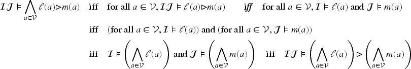
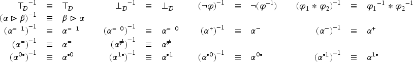
For $φ \in Δ L P$ , let $φ^{- 1} \in Δ L P$ semantically defined by
$M (φ^{- 1}) = {J I | I J \in M (φ)}$

The following proposition shows how $φ^{- 1}$ can be syntactically defined, whatever the choice of syntactic constructors of $(Δ L P, ⊨)$ are chosen according to Proposition 4:
Proposition 7
Let $α, β \in L P$ , $ψ, φ_{1}, φ_{2} \in Δ L P$ and $* \in {\land, \lor, \to, \leftrightarrow}$ . Then:
$\begin{array}{rclcrclcrclcrcl} {⊤_{D}}^{- 1} & \equiv & ⊤_{D} & {⊥_{D}}^{- 1} & \equiv & ⊥_{D} & {(\neg φ)}^{- 1} & \equiv & \neg (φ^{- 1}) & {(φ_{1} * φ_{2})}^{- 1} & \equiv & {φ_{1}}^{- 1} * {φ_{2}}^{- 1} \\ {(α ▹ β)}^{- 1} & \equiv & β ▹ α \\ {(α^{= 1})}^{- 1} & \equiv & α^{= 1} & {(α^{= 0})}^{- 1} & \equiv & α^{= 0} & {(α^{+})}^{- 1} & \equiv & α^{-} & {(α^{-})}^{- 1} & \equiv & α^{+} \\ {(α^{=})}^{- 1} & \equiv & α^{=} & {(α^{\neq \neq})}^{- 1} & \equiv & α^{\neq \neq} \\ {(α^{0 ∙})}^{- 1} & \equiv & α^{∙ 0} & {(α^{1 ∙})}^{- 1} & \equiv & α^{∙ 1} & {(α^{∙ 0})}^{- 1} & \equiv & α^{0 ∙} & {(α^{∙ 1})}^{- 1} & \equiv & α^{1 ∙} \end{array}$

Proof Sketch of proof.

The proof of each of these equivalences is rather straightforward. As an example, the equivalence ${(\neg φ)}^{- 1} \equiv \neg (φ^{- 1})$ can be proven as follows (for $I J \in Δ Ω$ ):

\begin{aligned} I J ⊨ {(\neg φ)}^{- 1} iff J I ⊨ \neg φ iff J I ⊭ φ iff I J ⊭ φ^{- 1} iff I J ⊨ \neg (φ^{- 1}) \end{aligned}

3.4.2 Composition of Two Formulas

Definition 4
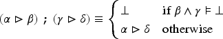
Let $φ, ψ \in Δ L P$ . The composition of $φ$ and $ψ$ is a formula $φ; ψ$ defined semantically by
$M (φ; ψ) = {I K \in Δ Ω \begin{array}{l} ~there exists J \in Ω such that I J ⊨ φ and J K ⊨ ψ \end{array}}$

In other words, $M (φ; ψ)$ is the composition of the binary relations $M (φ)$ and $M (ψ)$ on $Ω$ : $M (φ; ψ) = M (ψ) \circ M (φ)$ .

The following result is a direct consequence of associativity of binary relation composition:
$\begin{aligned} for φ, ψ, χ \in Δ L P, (φ; ψ); χ \equiv φ; (ψ; χ) \end{aligned}$
This allows to omit parentheses in compositions.

The research of a formula equivalent to $φ; ψ$ is studied via the following propositions, whose proofs are given in Appendix Section A.2.

Let us start with the case where the formulas to be composed are of the form $α ▹ β$ .
Proposition 8
Let $α, β, γ, δ \in L P$ . Then:
$(α ▹ β); (γ ▹ δ) \equiv {\begin{cases} ⊥ & if β \land γ ⊨ ⊥ \\ α ▹ δ & otherwise \end{cases}$

We focus next on the links between composition and disjunction:
Proposition 9
Let $φ, φ_{1}, φ_{2}, ψ, ψ_{1}, ψ_{2} \in Δ L P$ . The following equivalences hold:
$\begin{aligned} φ; (ψ_{1} \lor ψ_{2}) & \equiv (φ; ψ_{1}) \lor (φ; ψ_{2}) \end{aligned}$
(8)

$\begin{aligned} (φ_{1} \lor φ_{2}); ψ & \equiv (φ_{1}; ψ) \lor (φ_{2}; ψ) \end{aligned}$
(9)
Definition 5
Two additional variation symbols are introduced: $⊥_{D}$ and $⊤_{D}$ such that, for all $α \in L P$ , $α^{⊥_{D}} = ⊥ ▹ ⊥ = ⊥_{Δ}$ and $α^{⊤_{D}} = ⊤ ▹ ⊤ = ⊤_{Δ}$ .

To a variable $x$ and a cube $φ$ of $(Δ L P, ⊨)$ is associated $var (x, φ) \in D \cup {⊤_{D}}$ as follows:
$var (x, φ) = {\begin{cases} ⊤_{D} & if x \notin V (φ) \\ v & if x^{v} is a term of φ \end{cases}$

The following proposition allows to compute the composition of two literals of $(Δ L P, ⊨)$ built on the same variable.
Proposition 10
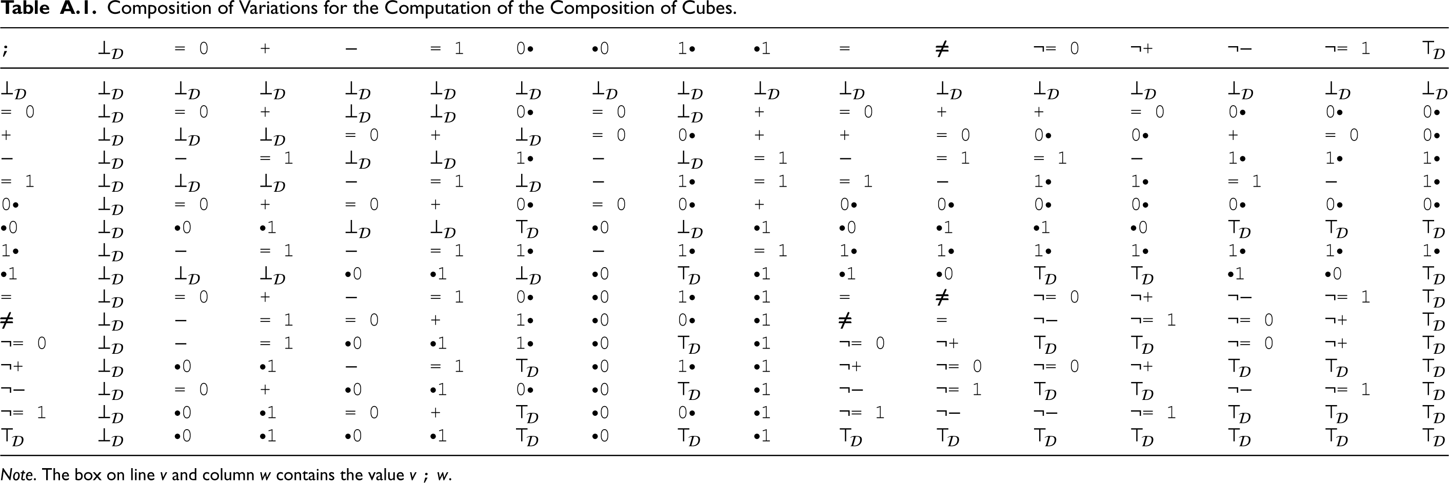
There exists a binary operation $;$ over $D \cup {⊥_{D}, ⊤_{D}}$ such that for $a \in V$ and $v, w \in D \cup {⊥_{D}, ⊤_{D}}$ , $a^{v}; a^{w} = a^{v; w}$ .

Now, the composition of cubes can be computed thanks to the following proposition:
Proposition 11
Let $φ$ and $ψ$ be two cubes of $(Δ L P, ⊨)$ . Then
$\begin{aligned} φ; ψ \equiv \underset{a \in V}{⋀} a^{var (a, φ); var (a, ψ)} \end{aligned}$
(10)

To compose two cubes, Proposition 11 is applied and then a simplification is made by remembering that $x^{⊤_{D}} \equiv ⊤$ and $x^{⊥_{D}} \equiv ⊥$ . For example, if the set of variables is ${a, b, c, d, e}$ then, according to Table 2 in Appendix Section A.2:
$\begin{aligned} a^{+} \land b^{=} \land d^{= 0}; a^{-} \land c^{-} \land d^{+} \equiv a^{= 0} \land b^{⊤_{D}} \land c^{∙ 0} \land d^{+} \land e^{⊤_{D}} \equiv a^{= 0} \land c^{∙ 0} \land d^{+} \end{aligned}$

More generally, a way to have a syntactical expression of $φ; ψ$ consists in putting these two formulas of $(Δ L P, ⊨)$ under DNF, and then applying the equivalences of Proposition 9 as long as it is possible, and finally applying Proposition 11 to eliminate completely the symbol $;$ .
4. A Sound and Complete Formal System for $(Δ L P, ⊨)$

In this section, $S_{Δ H}$ , a formal system sound and complete for $(Δ L P, ⊨)$ is presented and studied that is strongly inspired by $S_{H}$ , the formal system of Hilbert that is sound and complete for $(L P, ⊨)$ .

4.1. Definition of the Formal System $S_{Δ H}$

$S_{Δ H}$ , as any Hilbert style formal system, is defined by a triple $(L_{S_{Δ H}}, A_{S_{Δ H}}, {I R}_{S_{Δ H}})$ where $L_{S_{Δ H}}$ is the set of the well-formed formulas (wffs) of $S_{Δ H}$ , $A_{S_{Δ H}}$ is the set of its axioms and ${I R}_{S_{Δ H}}$ is the set of its inference rules.

Proposition 4 shows that every formula can be written with some syntactical restrictions. In particular, every formula can be written only with the atoms $a^{v}$ where $a \in V$ and $v \in D_{0}$ , and with the only connectives $\neg$ and $\to$ (the other connectives being defined as abbreviations, e.g., $φ \land ψ$ is an abbreviation for $\neg (φ \to \neg ψ)$ ). A wff $φ \in L_{S_{Δ H}}$ is a formula of $Δ L P$ with these syntactical restrictions.

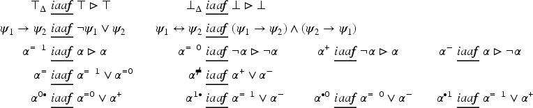
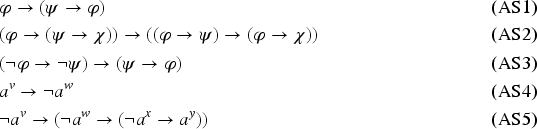
The set of axioms, $A_{S_{Δ H}}$ , is a subset of $L_{S_{Δ H}}$ defined by the following axiom schemes:

\begin{aligned} {(AS1)} & φ \to (ψ \to φ) \\ {(AS2)} & (φ \to (ψ \to χ)) \to ((φ \to ψ) \to (φ \to χ)) \\ {(AS3)} & (\neg φ \to \neg ψ) \to (ψ \to φ) \\ {(AS4)} & a^{v} \to \neg a^{w} \\ {(AS5)} & \neg a^{v} \to (\neg a^{w} \to (\neg a^{x} \to a^{y})) \end{aligned}

where

φ

ψ

, and

χ

have to be replaced with any wffs,

a

has to be replaced with any variable, and

v

w

x

y

have to be replaced by primitive variation symbols that are pairwise distinct. The axioms schemes (AS1), (AS2), and (AS3) are directly taken from Hilbert formal system. The axiom schemes (AS4) and (AS5) translate the fact that

{M (a^{v}) | v \in D_{0}}

is a partition of

Δ Ω

${I R}_{S_{Δ H}} = {m p}$ : the only inference rule of $S_{Δ H}$ is the modus ponens that is also the only inference rule of $S_{H}$ : $\frac{φ φ \to ψ}{ψ} m p$ .

4.2. Soundness of $S_{Δ H}$ for $(Δ L P, ⊨)$

Let $⊢^{Δ}$ be the entailment relation associated with $S_{Δ H}$ whose definition is recalled now. Let $B$ be a subset of $L_{S_{Δ H}}$ and $φ \in Δ L P$ . A proof of $φ$ from $B$ is a finite sequence $φ_{1}, φ_{2}, \dots, φ_{p}$ such that $φ_{p} = φ$ and, for each $k \in {1, 2, \dots, p}$ , $φ_{k}$ is either an axiom, or an element of $B$ , or is obtained by application of the inference rule on formulas $φ_{ℓ}$ where $ℓ < k$ . Then, $B ⊢^{Δ} φ$ is defined by the existence of a proof of $φ$ from $B$ .

Proposition 12
The formal system $S_{Δ H}$ is sound for $(Δ L P, ⊨)$ : for every finite set $B$ of wffs of $S_{Δ H}$ and every $φ \in L_{S_{Δ H}}$ , $if B ⊢^{Δ} φ then B ⊨ φ$ .
Proof Sketch of proof.

The soundness is proven in the usual way. First, it is shown that every axiom of $S_{Δ H}$ is a tautology of $(Δ L P, ⊨)$ . Then, the soundness of modus ponens is shown: if $I J$ is a model of $φ$ and of $φ \to ψ$ (for $φ$ and $ψ$ , two wffs) then $I J$ is a model of $ψ$ . Using these two results, it is shown by mathematical induction that, if $φ_{1}, φ_{2}, \dots, φ_{p}$ is a proof of $φ$ from $B$ and $I J ⊨ B$ then $I J ⊨ φ_{k}$ for each $k \in {1, 2, \dots, p}$ . So, $I J ⊨ φ$ (since $φ = φ_{p}$ ). Therefore, if $B ⊢^{Δ} φ$ then $B ⊨ φ$ .

4.3. Completeness of $S_{Δ H}$ for $(Δ L P, ⊨)$

Proposition 13
The formal system $S_{Δ H}$ is complete for $(Δ L P, ⊨)$ : for every finite set $B$ of wffs of $S_{Δ H}$ and every $φ \in L_{S_{Δ H}}$ , $if B ⊨ φ then B ⊢^{Δ} φ$ .

The proof of this result is given in Appendix Section A.3.
5. Algorithmic Issues

This section explores two algorithmic aspects of satisfiability in $Δ L P$ . First, it is shown that the problem ${SAT}_{Δ}$ of satisfiability in $Δ L P$ is NP-complete. Second, a semantic tableaux algorithm to test the satisfiability of a formula is presented.

5.1. Satisfiability Checking in $(Δ L P, ⊨)$ is NP-Complete

Let ${SAT}_{Δ}$ be the decision problem which, given a formula $φ$ of $(Δ L P, ⊨)$ , determines whether $φ$ is satisfiable. The problem ${SAT}_{Δ}$ is NP-complete. It is shown by proving that ${SAT}_{Δ}$ is in NP, then that it is NP-hard. The detailed proof is given in Appendix Section A.4.

5.2. A Semantic Tableaux Algorithm for Satisfiability Checking in $(Δ L P, ⊨)$

Semantic tableaux form a family of methods for satisfiability checking applicable to many logics (e.g., propositional logic and first order logic (Smullyan, 1995), and description logics (Baader & Sattler, 2001)). This section presents a semantic tableaux algorithm for $(Δ L P, ⊨)$ based on an adaptation of a semantic tableaux algorithm for $(L P, ⊨)$ .

5.2.1. Description of the Algorithm

Given a knowledge base $B$ of $(Δ L P, ⊨)$ and $φ \in Δ L P$ , the deduction test “ $B ⊨ φ$ ?” is equivalent to the test of unsatisfiability of $⋀ B \land \neg φ$ . So, deduction amounts to satisfiability checking.

The input of the algorithm is a formula $φ$ of $(Δ L P, ⊨)$ . Its output is the answer to the question “Is $φ$ satisfiable?”

The first step of the algorithm consists in putting $φ$ in NFNF (connectives $\land$ and $\lor$ , connective-free subformulas of the form $a^{v}$ , $a \in V$ , $v \in D_{0}$ ): the result of this step is a formula $ψ$ under NFNF such that $φ \equiv ψ$ .

The second step of the algorithm is the development of a tree $T r$ whose nodes are labeled by $(Δ L P, ⊨)$ formulas. A branch of such a tree is frequently assimilated in the following with the set $B$ of the formulas labeling the nodes of this branch.

The tree $T r$ of formulas is developed in the following way. Initially, $T r$ has only one node labeled by $ψ$ . Then, the following modifications of $T r$ are applied (the algorithm is non-deterministic: the order of application of these modifications changes neither the termination nor the result but has an impact on the computing time):

(A)
If a branch $B$ of $T r$ contains a conjunction $χ_{1} \land \dots \land χ_{p}$ such that for at least one $k \in {1, \dots, p}$ , $χ_{k} \notin B$ , then the tree is updated by extending $B$ with every $χ_{k} \notin B$ : the new value of the branch is $B \cup {χ_{1}, \dots, χ_{p}}$ .
(B)
If a branch $B$ of $T r$ contains a disjunction $χ_{1} \lor \dots \lor χ_{p}$ such that for every $k \in {1, \dots, p}$ , $χ_{k} \notin B$ , then the branch is “forked” in $p$ branches $B_{k} = B \cup {χ_{k}}$ .
The development of a branch $B$ is stopped if $B$ contains two literals $a^{v}$ and $a^{w}$ with $v \neq w$ , and then $B$ is said to end with the clash ${a^{v}, a^{w}}$ . It is also stopped if neither (A) nor (B) apply to the branch. In both cases, $B$ is said complete.

The algorithm stops when every branch of $T r$ is complete, and returns “ $φ$ is unsatisfiable” if every branch ends with a clash and “ $φ$ is satisfiable” otherwise.
5.2.2. Properties of the Algorithm

This algorithm always terminates (Proposition 14) and returns the expected result (according to Propositions 15 and 16). The proofs of these results are given in Appendix Section A.5.

Proposition 14
The tableau algorithm described in Section 5.2.1 always terminates.
Proposition 15
If the algorithm of Section 5.2.1 ends with a clash in every branch, then $φ$ is unsatisfiable.
Proposition 16
If $φ \in Δ L P$ is unsatisfiable then every complete tree $T r$ derived from the algorithm of Section 5.2.1 ends with a clash.
6. Application to CBR

The study of the logic $(Δ L P, ⊨)$ has been motivated by a notation used in CBR, a syntax that has not been associated with a semantics before. Now, this section presents an application of this logic to CBR that is centered on the notion of adaptation rule. Section 6.1 introduces an example of adaptation problem in CBR that can be solved thanks to the application of an adaptation rule. Section 6.2 describes the representation of adaptation rules. Such a rule is based on a formula of $(Δ L P, ⊨)$ and the handling of a rule is based on the notion of application of a variation formula on a propositional formula which is described in Section 6.5. This requires the notion of ceteris paribus which is introduced before, in Section 6.4, and this latter requires the notion of invariant variables of a formula, introduced even before, in Section 6.3. Then, the application of an adaptation rule on the example is described (Section 6.6). From this study, an algorithm for performing CBR (including retrieval and adaptation) based on the notion of adaptation rules is presented (Section 6.7). Finally, an open problem related to the composition of adaptation rules is presented in Section 6.8.

6.1. Introduction of an Example

An example in the cooking domain is considered: a problem represents a query of recipe and a solution, a recipe. The problems and solutions are assumed to be expressed in propositional logic. It is assumed in this example that the domain knowledge is empty: $DK = ⊤$ . The adaptation problem is $(c^{s}, x^{tgt})$ where

$c^{s}$ is the source case of a salad recipe, with batavia lettuce, duck filet, tomatoes, olive oil, and vinegar:

\begin{aligned} c^{s} = & rSalad \land {{i{BataviaLettuce}}} \land {{i{DuckFilet}}} \land {{i{Tomato}}} \\ \land {{i{OliveOil}}} \land {{i{Vinegar}}} \land n o t h i n g e l s e \end{aligned}

where

rSalad

is read “salad recipe,”

iSomething

, “recipe with the ingredient ‘something”’ and

n o t h i n g e l s e

is a notation for the conjunction of negative literals

\neg a

such that

a

cannot be deduced from the start of the formula:

α \land n o t h i n g e l s e \equiv α \land ⋀ {\neg a | a \in V and α ⧸ ⊨_{DK} a}

. In particular,

c^{s} ⊨_{DK} \neg {{i{Garlic}}}

. It can be noticed that

c^{s}

is a complete cube of propositional logic.

$x^{tgt}$ is the target problem “I want a recipe of salad with tomatoes, lemon juice but no garlic.”:

x^{tgt} = rSalad \land {{i{Tomato}}} \land {{i{LemonJuice}}} \land \neg {{i{Garlic}}}

Knowing the adaptation problem

(c^{s}, x^{tgt})

makes it possible to partition

V

{V_{P}, V_{S}}

V_{P} = V (x^{tgt}) = {rSalad, {{i{Tomato}}}, {{i{LemonJuice}}}, {{i{Garlic}}}}

and

V_{S} = V ∖ V_{P}

. Therefore,

c^{s}

can be written

c^{s} = x^{s} \land y^{s}

with

\begin{aligned} x^{s} & = rSalad \land {{i{Tomato}}} \land \neg {{i{LemonJuice}}} \land \neg {{i{Garlic}}} \\ y^{s} & = {{i{BataviaLettuce}}} \land {{i{DuckFilet}}} \land {{i{OliveOil}}} \land {{i{Vinegar}}} \land \dots \end{aligned}

(“

\dots

” corresponds to the conjunction of literals

\neg a

where

a \in V_{S}

and

a

is not a positive literal of

y^{s}

An itemset $I$ is also considered, that is obtained by an itemset extraction system (e.g., a frequent closed itemset system, see, e.g., Zaki and Hsiao (2002)) for the adaptation knowledge learning. Such an itemset contains a finite set of literals $a^{v}$ indicating “simultaneous” variations between cases and is interpreted by the conjunction $φ$ of its elements. $φ$ can be written as a cube of $(Δ L P, ⊨)$ : if there are several literals $a^{v_{1}}$ , $a^{v_{2}}$ , …built with the same variable $a$ that occur in $φ$ , it can be shown that they can be replaced with a sole $a^{v}$ (e.g., $a^{+} \land a^{\neq \neq} \land b^{1 ∙} \land b^{=} \equiv a^{+} \land b^{= 1}$ ). In the example, the following formula is considered:

φ = {rSalad}^{= 1} \land {{i{Vinegar}}}^{-} \land {{i{LemonJuice}}}^{+} \land {{i{Salt}}}^{+}

The itemset $I$ from which $φ$ is built reflects the fact that there is a sufficient number of ordered pairs of salad recipes with vinegar in the first recipe but not in the second one, and lemon juice and salt in the second one but not in the first one. Therefore, if $φ$ is interpreted as an adaptation rule, then applicability and application of $φ$ on the adaptation problem $((x^{s}, y^{s}), x^{tgt})$ have to be studied.

6.2. Representing an Adaptation Rule

An adaptation rule is defined as a pair $AR = (φ, C)$ where $φ \in Δ L P$ and $C$ is a nonnegative real number called cost of $AR$ .

What does it mean that $AR$ is applicable to an adaptation problem $((x^{s}, y^{s}), x^{tgt})$ and how can the result of this application be defined? To answer these questions, a mapping is considered that associates to $(α, φ, γ) \in L P \times Δ L P \times L P$ a formula $appl (α, φ, γ) \in L P$ , the application on $α$ of $φ$ under constraint $γ$ . This mapping is defined and studied further. Since the source cases and the target problem have to be considered with the domain knowledge $DK$ , the following formula will be computed:

β = appl (DK \land x^{s} \land y^{s}, φ, DK \land x^{tgt})

(11)

β ⊨ ⊥

then

AR

is said to be non-applicable to the adaptation problem. Else, this result can be written

β \equiv DK \land x^{tgt} \land y^{tgt}

where

y^{tgt}

is the solution proposed for

x^{tgt}

by application of

AR

for this adaptation problem.

CBR is usually a hypothetical inference and adaptation does not necessarily produce a correct solution to the target problem. In particular, the application of an adaptation rule $AR = (φ, C)$ may output an incorrect solution. In order to make a selection among a set of adaptation rules applicable to the same adaptation problem, $C$ is used: the cost associated with a rule is indicative of the plausibility of the application of this rule. The higher the $C$ is, the least the confidence on the application of the rule will be. For instance, this can be interpreted in a probabilistic setting: if $P$ estimates the probability that a rule produces a correct result (under some given probability distribution), then $C = - \log P$ could be a reasonable choice.

Thus, the representation of an adaptation rule amounts to the definition of the $appl$ mapping, which requires preliminary definitions presented in the next two sections.

Before that, a preliminary remark on the representation of source cases $(x^{s}, y^{s})$ and on adaptation rules $(φ, C)$ is made: although the study that follows makes no theoretical restriction on the form of source cases and adaptation rules, a reasonable assumption is that $x^{s}$ , $y^{s}$ , and $φ$ are cubes, and that justifies that these situations are considered with some importance. Since a source case $(x^{s}, y^{s})$ usually represents a specific problem-solving episode, it means that every (problem or solution) variable $a$ is assigned a Boolean value for this case: either $x^{s} \land y^{s} ⊨ a$ or $x^{s} \land y^{s} ⊨ \neg a$ , so $x^{s}$ and $y^{s}$ can both be written as cubes. For $φ$ , if it is obtained by a frequent itemset extraction system, then $φ = ⋀ I$ for an itemset $I$ which is a set of literals $a^{v}$ , and so, $φ$ is a cube.

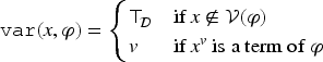
6.3. Invariant Variables of a Variation Formula

In this section, the variables that leave a formula unchanged are defined. The subset $Inv (φ)$ of $V$ is defined using the alternative definition of the semantics of $(Δ L P, ⊨)$ introduced in Section 3.2.2. The idea is that $a \in Inv (φ)$ means that the value of $ω (a)$ does not influence the satisfiability of $φ$ by $ω$ , for any $ω \in {Δ Ω}_{alt}$ . Formally, this leads to the following definition:

Definition 6
For $ω \in {Δ Ω}_{alt}$ , $a \in V$ and $v \in D_{0}$ , $ω [a^{v}] \in {Δ Ω}_{alt}$ is defined by $ω [a^{v}] : x \in V \mapsto {\begin{cases} v & if x = a \\ ω (x) & else \end{cases}$ .

For $φ \in Δ L P$ , the set of invariant variables of $φ$ is
$Inv (φ) = {a \in V | forevery ω \in M_{alt} (φ) and every v \in D_{0}, ω [a^{v}] ⊨_{alt} φ}$

For example,
$if V = {a, b, c} and φ = (a^{+} \land b^{=}) \lor (a^{+} \land b^{+}) \lor (a^{+} \land b^{-}) then Inv (φ) = {b, c}$
(12)

This notion is independent from syntax: if $φ \equiv ψ$ then $Inv (φ) = Inv (ψ)$ . It can be shown, using Lemma 1, that if a variable $x$ does not occur in $φ$ then it is invariant. Thus:
$V ∖ V (φ) \subseteq Inv (φ) \subseteq V$
(13)

As example (12) shows, a variable occurring in $φ$ can be invariant for $φ$ . The following proposition shows that a formula transformation makes it possible to link more tightly non-occurrences of variables to $Inv (φ)$ .
Proposition 17
For every $φ \in Δ L P$ , there exists $φ^{'} \in Δ L P$ such that $φ \equiv φ^{'}$ and $Inv (φ) = V ∖ V (φ^{'})$ .
Proof.
First, the case where $Inv (φ) = \emptyset$ is considered. In this case, the result is immediately verified with $φ^{'} = φ$ as an immediate consequence of (13).

Then, the case where $Inv (φ) = {a_{1}}$ is considered. $φ$ can be put under the form of a disjunction of complete cubes: $φ \equiv φ_{0}$ with $φ_{0} = \underset{ω \in M_{alt} (φ)}{⋁} φ_{ω} where φ_{ω} = \underset{x \in V}{⋀} x^{ω (x)}$ . Let $ω \in M_{alt} (φ)$ . By definition of $Inv (φ)$ , $ω [a_{1}^{v}] \in M_{alt} (φ)$ , for all $v \in D_{0}$ . Therefore, as soon as a $φ_{ω}$ occurs in the disjunction $φ_{0}$ , every $φ_{ω [a_{1}^{v}]}$ for $v \in D_{0}$ occur in $φ_{0}$ . Then, by repeating and gathering elements in the disjunction (which is possible since $\lor$ is associative and commutative modulo logical equivalence and $ψ \equiv ψ \lor ψ$ for every formula $ψ$ ), it yields that:
$\begin{aligned} φ_{0} & \equiv \underset{ω \in M_{alt} (φ)}{⋁} \underset{v \in D_{0}}{⋁} \underset{x \in V}{⋀} x^{ω [a_{1}^{v}] (x)} \equiv \underset{ω \in M_{alt} (φ)}{⋁} \underset{v \in D_{0}}{⋁} [a_{1}^{ω [a_{1}^{v}] (a_{1})} \land \underset{x \in V ∖ {a_{1}}}{⋀} x^{ω [a_{1}^{v}] (x)}] \\ \equiv \underset{ω \in M_{alt} (φ)}{⋁} \underset{v \in D_{0}}{⋁} [a_{1}^{v} \land \underset{x \in V ∖ {a_{1}}}{⋀} x^{ω (x)}] \equiv \underset{ω \in M_{alt} (φ)}{⋁} [\underset{x \in V ∖ {a_{1}}}{⋀} x^{ω (x)}] \land \underset{v \in D_{0}}{⋁} a_{1}^{v} \\ \equiv \underset{ω \in M_{alt} (φ)}{⋁} [\underset{x \in V ∖ {a_{1}}}{⋀} x^{ω (x)}] since \underset{v \in D_{0}}{⋁} a_{1}^{v} \equiv ⊤ \end{aligned}$
Let $φ_{1}$ be the last formula of the equivalence sequence above. Because $a_{1} \notin V (φ_{1})$ and $φ_{1} \equiv φ$ , the proposition is proven with $φ^{'} = φ_{1}$ .

In the case where $Inv (φ) = {a_{1}, a_{2}, \dots, a_{p}}$ , the process above can be applied on $φ$ in order to obtain $φ_{1}$ such that $a_{1}$ does not occur in $φ_{1}$ , then, by repeating it with the set of variables $V ∖ {a_{1}}$ on $φ_{1}$ , the formula $φ_{2}$ is obtained, $φ_{2}$ being a formula equivalent to $φ$ with no occurrence neither of $a_{1}$ nor of $a_{2}$ . Then, the process is repeated to result in a formula $φ_{p}$ equivalent to $φ$ with no occurrence in $Inv (φ)$ . With $φ^{'} = φ_{p}$ , this concludes the proof of the proposition.

The particular case of the following proposition will be useful in the remainder of the article.
Proposition 18
If $φ$ is a cube of $(Δ L P, ⊨)$ then $Inv (φ) = V ∖ V (φ)$ .
Proof.
In this proof, for a cube $φ$ , $φ [a^{v}]$ is a cube such that if $a \notin V (φ)$ then $φ [a^{v}] = φ \land a^{v}$ , else, $φ [a^{v}]$ is obtained by replacing the conjunct $a^{w}$ of $φ$ by $a^{v}$ . Since $Inv (φ) \supseteq V ∖ V (φ)$ (cf. (13)), it is sufficient to show that if $a \in Inv (φ)$ then $a \notin V (φ)$ , which will be proven by contraposition. Let $a \in V (φ)$ . Let $v \in D$ be such that $a^{v}$ is a literal of $φ$ having $a$ as variable. Let $v_{0} \in D_{0}$ be such that $a^{v_{0}} ⊨ a^{v}$ (if $v$ is a primitive variation symbol, $v_{0} = v$ , else, there are several possible choices for $v_{0}$ , e.g., if $v = \neq \neq$ then $v_{0} = +$ ou $v_{0} = -$ can be chosen). Let $w \in D_{0} ∖ {v_{0}}$ . Then $φ [a^{v_{0}}] ⊨ a^{v_{0}}$ and $φ [a^{w}] ⊭ a^{v_{0}}$ (because, by hypothesis on the cubes, a variable occurs at most once in a cube which involves that cubes are satisfiable). Therefore, $φ [a^{v_{0}}] ≢ φ [a^{w}]$ and so $a \notin Inv (φ)$ .
6.4. Operator Ceteris Paribus

Consider the formula $a^{+}$ : it indicates that $a$ “goes” from $0$ to $1$ , the other variables being free to vary in any way. So, if $V = {a, b}$ then $M (a^{+}) = {(\bar{a} \bar{b}, a \bar{b}), (\bar{a} \bar{b}, a b), (\bar{a} b, a \bar{b}), (\bar{a} b, a b)}$ . It appears useful in some cases to express for example that $a$ goes from $0$ to $1$ , the other variables remaining unchanged. For this purpose, this will be expressed by a formula $cp (a^{+})$ that, with the example with two variables, gives $M (cp (a^{+})) = {(\bar{a} \bar{b}, a \bar{b}), (\bar{a} b, a b)}$ : in the models of this formula, $b$ “stays” at $0$ or “stays” at $1$ ( $cp$ stands for ceteris paribus, i.e., “All things being equal”), in other terms, $cp (a^{+}) ⊨ b^{=}$ . In this example, $b$ is a variable whose interpretation does not change the interpretation of $φ$ : $b \in Inv (φ)$ .

More generally, an operator $cp$ is searched for such that, for $φ, ψ \in Δ L P$ :

\begin{aligned} cp (φ) ⊨ φ \end{aligned}

(14)

\begin{aligned} for all x \in Inv (φ), cp (φ) ⊨ x^{=} \end{aligned}

(15)

\begin{aligned} if φ \equiv ψ then cp (φ) \equiv cp (ψ) \end{aligned}

(16)

\begin{aligned} if φ is satisfiable then cp (φ) is also satisfiable \end{aligned}

(17)

The following definition of $cp$ is proposed and then, it is proven that it satisfies these properties and that $cp (φ)$ is the most general formula (according to $⊨$ ) satisfying these properties.

Definition 7

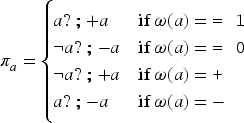
$cp$ is the mapping from $Δ L P$ to $Δ L P$ defined, for $φ \in Δ L P$ by

cp (φ) = φ \land ⋀ {x^{=} | x \in Inv (φ)}

Proposition 19

$cp$ satisfies (14), (15), (16), and (17). Moreover, if $φ^{'}$ satisfies these properties then $φ^{'} ⊨ cp (φ)$ .

Proof.

Equations (14), (15), and (16) follow immediately from the definition.

Equation (17) can be proven in the following way. Suppose $φ$ is satisfiable. Then it is also satisfiable according to the alternative definition of the semantics: there exists $ω \in {Δ Ω}_{alt}$ such that $ω ⊨_{alt} φ$ . Let $a_{1}$ , $a_{2}$ ,…, $a_{p}$ be such that $Inv (φ) = {a_{1}, a_{2}, \dots, a_{p}}$ . Let $ω^{'} = ω [a_{1}^{= 1}] [a_{2}^{= 1}] \dots [a_{p}^{= 1}]$ . By definition of $Inv (φ)$ , $ω^{'} ⊨_{alt} φ$ . Besides, $ω^{'} ⊨_{alt} a_{k}^{= 1}$ for all $k \in {1, 2, \dots, p}$ and so $ω^{'} ⊨_{alt} ⋀ {x^{= 1} | x \in Inv (φ)}$ . Now, for every variable $a$ , $a^{= 1} ⊨ a^{=}$ . Therefore, $ω^{'} ⊨_{alt} ⋀ {x^{=} | x \in Inv (φ)}$ . So, $ω^{'} ⊨_{alt} cp (φ)$ and so, $cp (φ)$ is satisfiable.

Now, let $φ^{'} \in Δ L P$ verifying the properties (14), (15), (16), and (17) of $cp (φ)$ . Then, according to (14) and (15), $φ^{'} ⊨ φ \land ⋀ {x^{=} | x \in Inv (φ)} = cp (φ)$ .

An immediate consequence of Proposition 18 is:

if φ is a cube then cp (φ) = φ \land \underset{x \in V ∖ V (φ)}{⋀} x^{=}

(18)

Moreover, the models of

cp (⊤)

are the

I I

for

I \in Ω

It can be noted that $cp$ is non-monotonic in the sense that for some $φ$ , $φ ⊨ ψ$ and $cp (φ) ⊭ cp (ψ)$ . For example, $a^{+} ⊨ ⊤$ and $cp (a^{+}) ⊭ cp (⊤)$ .

A practical issue is raised with this operator: for $φ \in Δ L P$ , $| cp (φ) |$ is in $O (| φ | + n)$ where $n = | V |$ and this may involve a long computing time. This problem turns theoretical if the logical framework is extended to an infinite set of variables: the definition of $cp$ given above cannot be applied, formulas being necessarily of finite sizes. A future work to address this issue will be the study of a possible extension of the logic by a connective $cp$ (rather than an operator $cp$ ).

It is sometimes useful to restrain the ceteris paribus to a predefined set of variables, hence the following definition.

Definition 8

Let $W \subseteq V$ and $φ \in Δ L P$ . The ceteris paribus of $φ$ restrained to the set of variables $W$ is:

{cp}_{W} (φ) = φ \land ⋀ {x^{=} | x \in Inv (φ) \cap W}

And, of course, ${cp}_{V} (φ) = cp (φ)$ .

6.5. Applying a Variation Formula to a Propositional Formula

This section aims at defining a notion of application of a formula $φ \in Δ L P$ to a formula $α \in L P$ , given an integrity constraint $γ \in L P$ on the result.

The application of $φ$ on $α$ under constraint $γ$ is denoted $appl (α, φ, γ)$ in the following (as mentioned in Section 6.2). In order to reach its definition, first, a formula $transf (α, φ, γ) \in Δ L P$ is considered, called the transformation of $α$ by $φ$ under constraint $γ$ , and whose result (its right part, obtained by application of the operator $R$ ) will be $appl (α, φ, γ) = R (transf (α, φ, γ))$ .

The three following conditions are proposed for an $I J \in Δ Ω$ to be a model of $transf (α, φ, γ)$ : $I ⊨ α$ , $I J ⊨ φ$ and $J ⊨ γ$ . These three conditions can be written as one:

I J ⊨ (α ▹ γ) \land φ

(19)

Is this condition sufficient? To answer this question, let us consider the following example:

α = a \land \neg b \land c

φ = a^{-} \land b^{+}

, and

γ = ⊤

. If (19) was a necessary and sufficient condition for

I J ⊨ transf (α, φ, γ)

then

appl (α, φ, γ)

would be equivalent to

R (φ)

, that is, to

\neg a \land b

. So, whether

α ⊨ c

α ⊨ \neg c

would not change the application of

φ

α

. On the contrary, it is assumed that if a variable (in this example

c

) is invariant in

φ

, its value should not be changed by the transformation, hence the use of the ceteris paribus (and an a posteriori justification of its study): so, it is assumed that

I J ⊨ cp (φ)

. The idea is that the formula

φ

represents in a compact manner a transformation and that when it expresses nothing about a variable

x

, this latter is unchanged by the transformation: if

x \in Inv (φ)

and

α ⊨ x

(resp.

α ⊨ \neg x

) then, with

β = appl (α, φ, γ)

β ⊨ x

(resp.

β ⊨ \neg x

). This leads to the following definition:

Definition 9

For $φ \in Δ L P$ and $α, γ \in L P$ , the transformation of $α$ by $φ$ under constraint $γ$ is defined by:

transf (α, φ, γ) = (α ▹ γ) \land cp (φ)

The application of

φ

α

under constraint

γ

is the result of this transformation:

appl (α, φ, γ) = R (transf (α, φ, γ))

φ

is said to be applicable on

α

under constraint

γ

appl (α, φ, γ) ⊭ ⊥

. Two necessary (but not sufficient) conditions of applicability are

α \land L (φ) ⊭ ⊥

and

R (φ) \land γ ⊭ ⊥

Despite the use of the ceteris paribus, if $α$ , $φ$ , and $γ$ contain few variables (wrt to $| V |$ ), the computation of $appl (α, φ, γ)$ can be performed without considering all the variables of $V$ , as shown in the following proposition:

Proposition 20

Let $α, γ \in L P$ and $φ \in Δ L P$ , and let $W = V (α) \cup V (φ) \cup V (γ)$ . Then

appl (α, φ, γ) \equiv R ((α ▹ γ) \land {cp}_{W} (φ))

Proof.

Let $β_{1} = appl (α, φ, γ) = R ((α ▹ γ) \land cp (φ))$ and $β_{2} = R ((α ▹ γ) \land {cp}_{W} (φ))$ . The goal is to prove that $β_{1} \equiv β_{2}$ .

Since $cp (φ) ⊨ {cp}_{W} (φ)$ , it can be deduced that $β_{1} ⊨ β_{2}$ (in particular because if $ψ ⊨ ψ^{'}$ then $R (ψ) ⊨ R (ψ^{'})$ for every $ψ \in Δ L P$ ).

Let us show that $β_{2} ⊨ β_{1}$ . Let $J \in M (β_{2})$ : what remains to be shown is that $J ⊨ β_{1}$ . By definition of $β_{2}$ , there exists $I \in Ω$ such that $I J ⊨ (α ▹ γ) \land {cp}_{W} (φ)$ . Then, let $I^{'} \in Ω$ defined (for $x \in V$ ) by $I^{'} (x) = {\begin{cases} I (x) & if x \in W \\ J (x) & else \end{cases}$ . It will be shown that $I^{'} J ⊨ (α ▹ γ) \land cp (φ)$ , which implies that $J ⊨ β_{2}$ . For this purpose, it is sufficient to show the following assertions: (A1)

$I^{'} J ⊨ α ▹ γ$ ;

(A2)

$I^{'} J ⊨ φ$ ;

(A3)

For all $x \in Inv (φ)$ , $I^{'} J ⊨ x^{=}$ .

Because the only difference between

I

and

I^{'}

concerns variables that are not in

V (α)

(since they are not in

W

) and because

I ⊨ α

, it yields that

I^{'} ⊨ α

. As

J ⊨ γ

, (A1) holds.

Similarly, the only difference between $I J$ and $I^{'} J$ concerns variables that are not in $V (φ)$ (since they are not in $W$ ) and because $I J ⊨ φ$ , it yields that $I^{'} J ⊨ φ$ , hence (A2).

Let $x \in Inv (φ)$ . To prove (A3), it is sufficient to prove that $I^{'} (x) = J (x)$ . If $x \notin W$ , by definition of $I^{'}$ , this holds. If $x \in W$ , $x \in Inv (φ) \cap W$ , so ${cp}_{W} (φ) ⊨ x^{=}$ (according to Definition 8). As $I J ⊨ {cp}_{W} (φ)$ , $I J ⊨ x^{=}$ , that is, $I (x) = J (x)$ . Now, $I^{'} (x) = I (x)$ since $x \in W$ . Therefore, $I^{'} (x) = J (x)$ , which proves (A3) and finishes the proof.

The following proposition gives a way to compute in $O (| V (α) | + | V (φ) | + | V (γ) |)$ the application of $φ$ on $α$ under constraint $γ$ when $α$ and $γ$ are cubes and $φ$ is a primitive cube.

Proposition 21

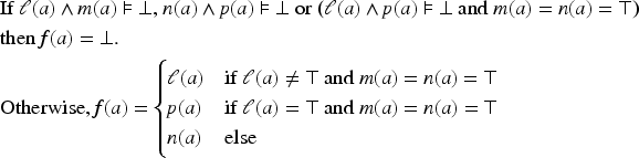
Let $α$ and $γ$ be two cubes of $(L P, ⊨)$ and $φ$ be a primitive cube of $(Δ L P, ⊨)$ . Let $W = V (α) \cup V (φ) \cup V (γ)$ . Thus, it is possible to write $α \equiv \underset{a \in W}{⋀} ℓ (a)$ , $γ \equiv \underset{a \in W}{⋀} p (a)$ , and $φ \equiv \underset{a \in W}{⋀} m (a) ▹ n (a)$ , where $ℓ (a)$ , $m (a)$ , $n (a)$ and $p (a)$ belong to ${a, \neg a, ⊤}$ , for every $a \in W$ . It can be noted that $a \in V (α)$ iff $ℓ (a) \neq ⊤$ , $a \in V (γ)$ iff $p (a) \neq ⊤$ and $a \in V (φ)$ iff $m (a) \neq ⊤$ or (equivalently) $n (a) \neq ⊤$ (since $φ$ is a primitive cube).

For $a \in W$ , $f (a) \in {a, \neg a, ⊥}$ is defined in the following way:

\begin{aligned} If ℓ (a) \land m (a) ⊨ ⊥, n (a) \land p (a) ⊨ ⊥ or (ℓ (a) \land p (a) ⊨ ⊥ and m (a) = n (a) = ⊤) \\ then f (a) = ⊥ . \\ Otherwise, f (a) = {\begin{cases} ℓ (a) & if ℓ (a) \neq ⊤ and m (a) = n (a) = ⊤ \\ p (a) & if ℓ (a) = ⊤ and m (a) = n (a) = ⊤ \\ n (a) & else \end{cases} \end{aligned}

Then

appl (α, φ, γ) \equiv \underset{a \in W}{⋀} f (a)

Therefore, $φ$ is applicable on $α$ under constraint $γ$ iff for all $a \in W$ , $f (a) \neq ⊥$ .

Proof Sketch of proof.

The idea of the proof consists in computing $appl (α, φ, γ)$ for every variable $a \in W$ . Indeed, $transf (α, φ, γ)$ can be written as a conjunction over $a \in W$ as shown below:

transf (α, φ, γ) = (α ▹ γ) \land cp (φ) \equiv \underset{a \in W}{⋀} (ℓ (a) ▹ p (a)) \land φ (a) where φ (a) = {\begin{cases} m (a) ▹ n (a) & if a \in V (φ) \\ a^{=} & else \end{cases}

The complete proof consists in considering all the possibilities for a variable

a \in W

, depending on whether

a

belongs or not to

V (α)

, to

V (φ)

and to

V (γ)

. So, there are

2^{3} = 8

cases to consider, but since

a \in W

, one of these cases is removed. Below, only two cases are detailed:

Case 1:
$a \in V (α)$ , $a \notin V (φ)$ and $a \notin V (γ)$ . Then $ℓ (a) \neq ⊤$ and $m (a) = n (a) = p (a) = ⊤$ . So:
$(ℓ (a) ▹ p (a)) \land φ (a) = (ℓ (a) ▹ ⊤) \land a^{=} \equiv ℓ (a) ▹ ℓ (a)$

Case 2:
$a \in V (α) \cap V (γ) \cap V (φ)$ . Then $⊤ \notin {ℓ (a), m (a), n (a), p (a)}$ , so:
$(ℓ (a) ▹ p (a)) \land φ (a) = (ℓ (a) ▹ p (a)) \land (m (a) ▹ n (a)) \equiv {\begin{cases} ℓ (a) ▹ n (a) & if ℓ (a) = m (a) and p (a) = n (a) \\ ⊥ & else \end{cases}$

The five remaining cases are studied similarly and this leads to the conclusion of the proposition.

Finally, the following proposition makes it possible to compute $appl (α, φ, γ)$ where $φ$ is a primitive cube but where $α$ and $γ$ are any propositional formulas, using transformations under disjunctive normal form of $α$ and $γ$ and Proposition 21.
Proposition 22
Let $α, α_{1}, α_{2}, β, β_{1}, β_{2} \in L P$ and $φ \in Δ L P$ . The following equivalences apply:
$\begin{aligned} appl (α_{1} \lor α_{2}, φ, γ) & \equiv appl (α_{1}, φ, γ) \lor appl (α_{2}, φ, γ) \end{aligned}$
(20)

$\begin{aligned} appl (α, φ, γ_{1} \lor γ_{2}) & \equiv appl (α, φ, γ_{1}) \lor appl (α, φ, γ_{2}) \end{aligned}$
(21)
Proof.
Equivalence (20) can be proven using Proposition 6(4), Section 3.3.4, and the following sequence of equivalences:
$\begin{aligned} transf (α_{1} \lor α_{2}, φ, γ) & = ((α_{1} \lor α_{2}) ▹ γ) \land cp (φ) \equiv ((α_{1} ▹ γ) \land cp (φ)) \lor ((α_{2} ▹ γ) \land cp (φ)) \\ \equiv transf (α_{1}, φ, γ) \lor transf (α_{2}, φ, γ) \end{aligned}$
Equivalence (21) can be proven in a similar way.
6.6. Application of an Adaptation Rule to the Example

Consider the adaptation problem $((x^{s}, y^{s}), x^{tgt})$ and the formula $φ$ of Section 6.1, along with the adaptation rule $AR = (φ, C)$ where $C$ is chosen arbitrarily. By applying (11) to this example, a satisfiable $β \in L P$ is obtained, and verifies $β \equiv DK \land x^{tgt} \land y^{tgt}$ with

y^{tgt} = {{i{BataviaLettuce}}} \land {{i{DuckFilet}}} \land {{i{OliveOil}}} \land {{i{LemonJuice}}} \land {{i{Salt}}} \land \dots

which is the expected result on this example (“

\dots

” represents a conjunction of negative literals).

6.7. An Algorithm for CBR

An approach to CBR used in particular in the system $Taaable$ (Cordier et al., 2014), consists in performing a retrieval relying on a minimal transformation of the target problem, such that it corresponds exactly to at least one source case, then using an “inverse transformation” on a retrieved case to obtain a solution.

In the representation setting of this article, the transformation of the target problem is built thanks to adaptation rules. Assume the adaptation knowledge of a CBR system is represented by the set $AK$ of available adaptation rules $(φ, C)$ . $AK$ may also contain the rules $(a^{\neq \neq}, C)$ for each problem variable $a$ : such a rule states that, given an adaptation problem $((x^{s}, y^{s}), x^{tgt})$ such that the only difference between the two problems $x^{s}$ and $x^{tgt}$ is related to the value of $a$ , the solution $y^{s}$ is reused as such. The role of these additional adaptation rules $(a^{\neq \neq}, C)$ is to ensure that the system proposes a solution (possibly with a high adaptation cost).

In order to implement the proposed algorithm, the transformations considered apply to the target problem, so are based on the rule ${AR}^{- 1} = (φ^{- 1}, C)$ for each $AR = (φ, C) \in AK$ (where $φ^{- 1}$ is the inverse of $φ$ , as defined in Definition 3). Assuming that costs are additive, the retrieval returns not only an $(x^{s}, y^{s}) \in CB$ but also a sequence of rules ${AR}_{1}^{- 1}, {AR}_{2}^{- 1}, \dots, {AR}_{q}^{- 1}$ that relates the target problem to this retrieved case. Formally, let $x^{0}$ , $x^{1}$ , …, $x^{q}$ defined by $x^{0} = DK \land x^{tgt}$ and $x^{i} = appl (x^{i - 1}, {φ_{i}}^{- 1}, ⊤)$ , for $i \in {1, 2, \dots, q}$ and ${AR}_{i} = (φ_{i}, C_{i})$ . Then, the retrieved case is such that $x^{s} \land y^{s} ⊨_{DK} x^{q}$ and such that the transformation cost $\sum_{i = 1}^{q} C_{i}$ is minimal. Algorithmically, it amounts to a best-first search in a state space where states are propositional formulas, $x^{0}$ is the initial state, the goal is to have a state that matches at least one source case (which can be done efficiently if source cases are specific), the successors of a state being obtained by inverse adaptation rules ${AR}^{- 1}$ , and the search being controlled by the cost.

Once a source case $(x^{s}, y^{s})$ retrieved with an associated sequence of adaptation rules ${AR}_{1}^{- 1}$ , ${AR}_{2}^{- 1}$ ,…, ${AR}_{q}^{- 1}$ the idea is to apply the inverse sequence of these rules to $x^{s} \land y^{s}$ to solve $x^{tgt}$ : with $y^{q}$ such that $x^{s} \land y^{s} \equiv x^{q} \land y^{q}$ , $y^{q - 1}$ ,…, $y^{0}$ , are computed successively: for $i \in {q - 1, q - 2, \dots, 0}$ , $x^{i} \land y^{i} \equiv appl (x^{i + 1} \land y^{i + 1}, φ_{i + 1}, x^{i})$ . Then $y^{tgt}$ such that $DK \land x^{tgt} \land y^{tgt} \equiv x^{0} \land y^{0}$ is a proposition of solution of $x^{tgt}$ , adapted in q steps from the retrieved case. It can be noted that above, the $x^{i}$ (resp., the $y^{i}$ ) are not necessarily problems (resp. solutions). For example, $V (x^{0}) \supseteq V (DK)$ and $DK$ may contain variables from $V_{S}$ .

For such an adaptation to give a consistent result, the adaptation rules ${AR}_{i}$ must be applicable. This is ensured by the following proposition, in the case where $x^{s} \land y^{s}$ , $x^{tgt}$ and $φ_{i}$ are cubes:

Proposition 23
Let $α$ and $γ$ be two cubes of $(L P, ⊨)$ and $φ$ be a cube of $(Δ L P, ⊨)$ . Then:
$appl (α, φ, γ) ⊭ ⊥ iff appl (γ, φ^{- 1}, ⊤) \land α ⊭ ⊥$

Proof Sketch of proof.

The conditions for the direct computation have already been seen in Proposition 21.

For the “inverse” computation, it yields that:

transf (γ, φ^{- 1}, ⊤) \equiv \underset{a \in V}{⋀} \underset{τ_{γ, φ} (a)}{\underset{⏟}{(p (a) ▹ ⊤) \land cp (φ^{- 1}) (a)}} where cp (φ^{- 1}) (a) = {\begin{cases} n (a) ▹ m (a) & if a \in V (φ) \\ a^{=} & else \end{cases}

The computation of the right part of

τ_{γ, φ} (a)

, and its conjunction with

α

, are done the same way it was done in the proof of Proposition 21, partitioning the set of variables according to

V (α)

V (φ)

and

V (γ)

For example, if $a \in V (α) \cap V (φ) \cap V (γ)$ , $(p (a) ▹ ⊤) \land cp (φ^{- 1}) (a) = (p (a) ▹ ⊤) \land (n (a) ▹ m (a))$ .

The compatibility condition of this conjunction is $n (a) \land p (a) ⊭ ⊥$ . The right part of this term is then $m (a)$ , and the compatibility condition with $α$ is $ℓ (a) \land m (a) ⊭ ⊥$ . The same conditions are met in the direct computation.

This computation is done the same way in the six other cases, and it is easy (but tedious!) to check the equivalence: $appl (γ, φ^{- 1}, ⊤) \land α ⊭ ⊥$ iff $appl (α, φ, γ) ⊭ ⊥$ .

It can be shown that $x^{i} \land y^{i}$ is satisfiable for all $i \in {0, 1, \dots, q}$ by starting from the end:

$(i = q)$
Since, by definition, $x^{q} \land y^{q}$ is equivalent to the complete cube $x^{s} \land y^{s}$ and cubes are satisfiable, $x^{q} \land y^{q} ⊭ ⊥$ .
$(i = q - 1)$
$x^{q - 1} \land y^{q - 1} \equiv appl (x^{q} \land y^{q}, φ_{q}, x^{q - 1})$ that, according to Proposition 23, is satisfiable iff $β$ is satisfiable, with $β = appl (x^{q - 1}, {φ_{q}}^{- 1}, ⊤) \land x^{q} \land y^{q}$ . Now, by definition of $x^{q}$ , $β \equiv x^{q} \land x^{q} \land y^{q} \equiv x^{q} \land y^{q}$ , which is satisfiable (cf. case $(i = q)$ ), thus $β$ is satisfiable and hence $x^{q - 1} \land y^{q - 1} ⊭ ⊥$ .
$(i = q - 2)$
$x^{q - 2} \land y^{q - 2} \equiv appl (x^{q - 1} \land y^{q - 1}, φ_{q - 1}, x^{q - 2})$ that, according to Proposition 23, is satisfiable iff $β$ is satisfiable, with $β = appl (x^{q - 2}, {φ_{q - 1}}^{- 1}, ⊤) \land x^{q - 1} \land y^{q - 1}$ . Now, by definition of $x^{q - 1}$ , $β \equiv x^{q - 1} \land x^{q - 1} \land y^{q - 1} \equiv x^{q - 1} \land y^{q - 1}$ which is satisfiable (cf. case $(i = q - 1)$ ), thus $β$ is satisfiable and hence $x^{q - 2} \land y^{q - 2} ⊭ ⊥$ .
$(\dots)$
$(i = 0)$
$x^{0} \land y^{0} \equiv appl (x^{1} \land y^{1}, φ_{1}, x^{0})$ that, according to Proposition 23, is satisfiable iff $β$ is satisfiable, with $β = appl (x^{0}, {φ_{1}}^{- 1}, ⊤) \land x^{1} \land y^{1}$ . Now, by definition of $x^{1}$ , $β \equiv x^{1} \land x^{1} \land y^{1} \equiv x^{1} \land y^{1}$ which is satisfiable (cf. case $(i = 1)$ ), thus $β$ is satisfiable and hence $x^{0} \land y^{0} ⊭ ⊥$ .
Since $DK \land x^{tgt} \land y^{tgt} \equiv x^{0} \land y^{0}$ , $DK \land x^{tgt} \land y^{tgt}$ is satisfiable: adaptation gives a consistent result.

It can be noted that this algorithm can be used to solve an adaptation problem $((x^{s}, y^{s}), x^{tgt})$ (when a case $(x^{s}, y^{s})$ has already been chosen). For this purpose, it only requires to apply the algorithm to the singleton case base $CB = {(x^{s}, y^{s})}$ .

A final but important remark has to be made. In the system $Taaable$ , retrieval was based only on a minimum generalization of the literals of the target problem according to a taxonomy, that is a set of formulas $a \to b$ ( $a, b \in V$ ). Such generalization, expressed with the logic developed in this article, corresponds to adaptation rules $(a^{-} \land b^{= 1}, C)$ . After that, a first raw adaptation was proposed (following the inverse of these taxonomy-based adaptation rules). Then, a rule-based adaptation using more sophisticated rules was performed. With the algorithm presented above, retrieval and adaptation are more tightly linked: once retrieval is done, adaptation just follows backward the adaptation rule chain. Therefore, the retrieval of this algorithm follows a strong version of the adaptation-guided retrieval principle (AGR; Smyth & Keane, 1996). In the usual version of AGR, the retrieved case has to be adaptable. Here, not only is it adapted, but the retrieved case is the source case that requires the least adaptation effort (measured by the costs of adaptation rules) to solve the target problem. Moreover, for this algorithm, retrieval knowledge and adaptation knowledge coincide: the rules $(φ, C)$ are used both for retrieval and for adaptation.
6.8. Toward a Composition of Adaptation Rules

The algorithm of Section 6.7 relies on a sequence of applications of adaptation rules. The open issue that is raised here is the computation of a composition of adaptation rules: given two rules ${AR}_{1}$ and ${AR}_{2}$ , can a rule $AR$ be defined such that the application of $AR$ corresponds to the successive applications of ${AR}_{1}$ and ${AR}_{2}$ ? The composition of formulas introduced in Section 3.4 should be useful here, but no definitive answer to this question has been found at this time.

The interest in defining such a composition of rules would be to use it during the post-treatment of learning these rules. If, for example, a frequent closed itemset extraction system is used, a large number of itemsets $I$ that can be interpreted as adaptation rules $AR$ may be produced. If it was possible to find a minimal generating family for the composition of these rules, it would lower their number (and computing time) without changing the algorithm.

7. Discussion and Related Works

This section discusses some formalisms with connections with the logic of propositional variables presented in this article. Section 7.1 considers briefly several of these formalisms. Dynamic logics are considered separately, since they have stronger similarities with $(Δ L P, ⊨)$ . For discussing these similarities (and differences), two types of inferences are highlighted first, in Section 7.2, namely observations and actions. Then, on this basis, $(Δ L P, ⊨)$ is related with DL-PA, a dynamic logic with propositional variables (Section 7.3).

7.1. A Few Related Formalisms and Other Studies

The notion of propositional variation may evoke the notion of differences between Boolean functions that have been studied in the work of Thayse (1981). Indeed, a formula $(L P, ⊨)$ can be seen as a representation of a function from ${0, 1}^{| V |}$ to ${0, 1}$ . In Thayse work, the differences between two Boolean variables is calculated by an exclusive or and this work leads to a differential calculus on Boolean functions inspired from studies in analysis on real numbers (Taylor developments, etc.). However, considering the original goal of this work described in this article, that is, representing variations, useful in particular for CBR, the sole use of exclusive or appears insufficient. In particular, the symmetry of $\oplus$ ( $α \oplus β \equiv β \oplus α$ ) does not make it possible to express directed variations, for example, to distinguish going from $0$ to $1$ and going from $1$ to $0$ , whereas the variation symbols $+$ and $-$ makes this distinction.

The alternative definition of the semantics of $(Δ L P, ⊨)$ (Section 3.2.2) is based on the set of truth values $D_{0}$ . This motivates to study the relationships between $(Δ L P, ⊨)$ and the logic of Belnap (2019) which is also based on four truth values which are often represented by ordered pairs of Booleans. From a semantic viewpoint, the link is not straightforward since $(Δ L P, ⊨)$ is most of the time considered as a logic with two truth values (the alternative definition of the semantics has mainly been introduced for practical purpose). Moreover, the number $4$ of truth values is at the basis of Belnap–Dunn logic whereas, for variation logic, it appears only as a consequence of choosing propositional logic as a starting point to build this logic: other choices could have been made, which would have led to a set of primitive variations of cardinal different from four. Now, relations between these two logics could be investigated, in particular, at an algorithmic level. This study has not been carried out and constitutes a potential future work.

7.2. Observations and Actions

The mechanisms linked to adaptation presented in Section 6 can be divided into observations and actions. The observations occur during the adaptation knowledge learning process (described in Section 2.2) during which are observed variations between source cases. Given an adaptation rule $AR = (φ, C)$ and an adaptation problem $((x^{s}, y^{s}), x^{tgt})$ , the application of $AR$ on $((x^{s}, y^{s}), x^{tgt})$ can be seen as an action mechanism: a plausible solution $y^{tgt}$ of $x^{tgt}$ is created, starting from $(x^{s}, y^{s})$ . So, assimilating a case to a state and an adaptation rule to an action, an adaptation rule can be considered as the application of an action on a state, to reach a new state (knowing that this new state is constrained by $x^{tgt}$ ). The application of adaptation rules is an invitation to study action-related formalisms and inferences (cf. the synthesis Dupin de Saint-Cyr et al., 2020). In this framework, the actions are considered as deterministic: if an action is applicable on a state, it generates exactly one state. The next section studies the links between a dynamic logic and $(Δ L P, ⊨)$ .

A last remark can be done. A link between observations and epistemic actions (also studied in Dupin de Saint-Cyr et al., 2020) could be considered. However, the study of the links between observations as considered here (observing variations between cases) and the epistemic actions (acting for observing and acquiring/modifying knowledge about the current state) has not appear fruitful (or not yet).

7.3. $(Δ L P, ⊨)$ and DL-PA

DL-PA (dynamic logic of propositional assignments) is a dynamic logic whose atomic programs are assignments of propositional variables, that is, expressions $+ a$ and $- a$ for $a \in V$ , corresponding to assignment of $a$ by, respectively, $1$ and $0$ (Balbiani et al., 2013). Formulas of DL-PA are the propositional variables, formulas build with other formulas using the connectives of propositional logic, and the formulas of the form $⟨ π ⟩ α$ where $π$ is a program and $α$ is a formula. Programs are either atomic programs, or of one of the forms $π_{1};; π_{2}$ , $π_{1} \cup \cup π_{2}$ , $π^{*}$ , and $α ?$ (where $π$ , $π_{1}$ , and $π_{2}$ are programs and $α$ is a formula).

The semantics of a formula $α$ is given by a subset $M (α)$ of $Ω$ and the semantics of a program $π$ by a subset $M (π)$ of $Ω \times Ω = Δ Ω$ , which suggests to study the link between DL-PA programs and $(Δ L P, ⊨)$ formulas. This semantics is defined in an usual way for propositional variables and formulas build on connectives, and for the other formulas and for the programs, in the following way (for $a \in V$ , $α$ , a formula, $π$ , $π_{1}$ and $π_{2}$ , programs):

\begin{aligned} M (⟨ π ⟩ α) & = {I \in Ω \begin{array}{l} there exists J \in Ω such that I J ⊨ π and J ⊨ α \end{array}} \\ M (+ a) & = {I J \in Δ Ω \begin{array}{l} J ⊨ a and, for all b \in V ∖ {a}, I (b) = J (b) \end{array}} \\ M (- a) & = {I J \in Δ Ω \begin{array}{l} J ⊨ \neg a and, for all b \in V ∖ {a}, I (b) = J (b) \end{array}} \\ M (π_{1};; π_{2}) & = {I K \in Δ Ω \begin{array}{l} there exists J \in Ω such that I J ⊨ π_{1} and J K ⊨ π_{2} \end{array}} \\ M (π_{1} \cup \cup π_{2}) & = M (π_{1}) \cup M (π_{2}) \\ M (α ?) & = {I I | I \in M (α)} \end{aligned}

Finally,

I J ⊨ π^{*}

if there exists a sequence

I_{0}, I_{1}, \dots, I_{p}

(

p \geq 0

) such that

I_{0} = I

I_{p} = J

and

I_{k} I_{k + 1} ⊨ π

for all

k \geq 0

and

k < p

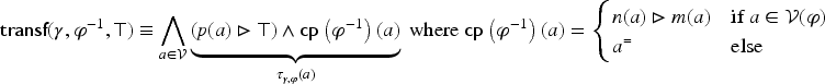
Ceteris paribus on $(Δ L P, ⊨)$ formulas is useful to establish a relationship from formulas of this logic to DL-PA programs. An operation on DL-PA programs can also be defined to establish a link in the other direction. For this purpose, it will be assumed in the remainder of this section that the set of propositional variables is finite, contrary to the assumption of a countable set of variables made in Balbiani et al. (2013).

It can be remarked that the program $+ a \cup \cup - a$ (for $a \in V$ ) does the opposite of an assignment: even if $a$ is assigned to a value ( $0$ or $1$ ) in the state preceding the application of this program, the execution of this program has for effect that $a$ does not have any assignment after this execution. This can be generalized to a set $W = {a_{1}, \dots, a_{p}}$ of variables:

unassign ({a_{1}, \dots, a_{p}}) = (+ a_{1} \cup \cup - a_{1});; \dots;; (+ a_{p} \cup \cup - a_{p})

The execution of

unassign (W)

has for effect that it reaches a state in which no variable of

W

has an assignment (so this state is a formula having at least

2^{| W |}

models).

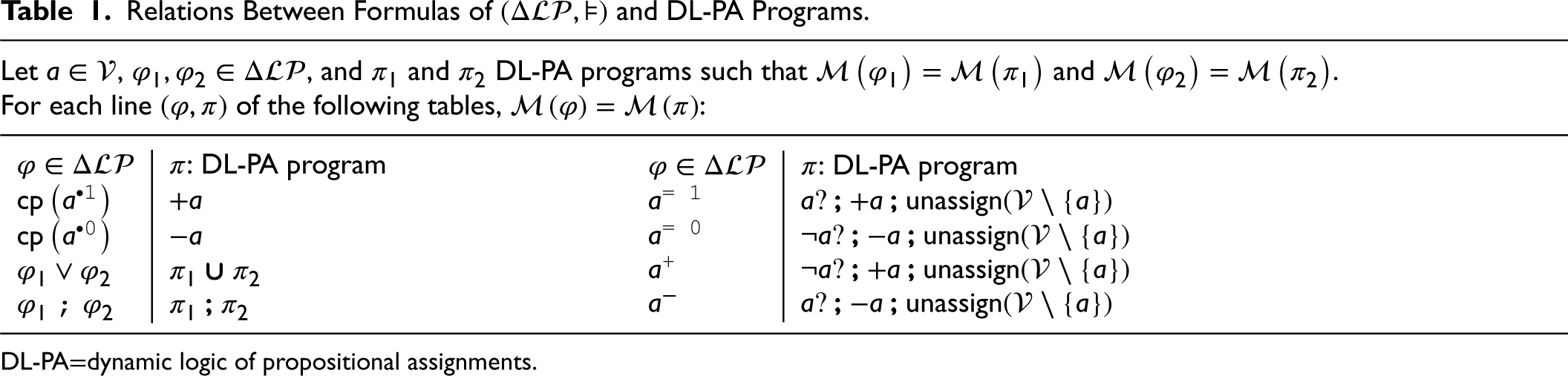
Table 1 gives equalities between sets of models of some formulas of $(Δ L P, ⊨)$ and set of models of some programs of DL-PA. It can be noted that, in this table, some operations of $(Δ L P, ⊨)$ correspond to constructors (syntactical elements) of DL-PA; for example, in $π_{1};; π_{2}$ the symbol $;;$ belongs to the syntax of the logic whereas in $φ_{1}; φ_{2}$ , $;$ is an operator. Moreover, for $α \in L P$ (which is also a formula of DL-PA), $M (α ?) = M (\hat{α})$ where $\hat{α}$ is defined in Appendix Section A.4, related to the proof of the NP-completeness of ${SAT}_{Δ}$ . Finally, for $α \in L P$ , $φ \in Δ L P$ , and a DL-PA program $π$ such that $M (φ) = M (π)$ , $M (⟨ π ⟩ α) = L (φ \land α^{∙ 1})$ .

Table 1.
Relations Between Formulas of $(Δ L P, ⊨)$ and DL-PA Programs.

Let $a \in V$ , $φ_{1}, φ_{2} \in Δ L P$ , and $π_{1}$ and $π_{2}$ DL-PA programs such that $M (φ_{1}) = M (π_{1})$ and $M (φ_{2}) = M (π_{2})$ .

For each line $(φ, π)$ of the following tables, $M (φ) = M (π)$ :

$\begin{array}{ll} φ \in Δ L P & π : DL-PA program \\ cp (a^{∙ 1}) & + a \\ cp (a^{∙ 0}) & - a \\ φ_{1} \lor φ_{2} & π_{1} \cup \cup π_{2} \\ φ_{1}; φ_{2} & π_{1};; π_{2} \end{array}$ $\begin{array}{ll} φ \in Δ L P & π : DL-PA program \\ a^{= 1} & a ?;; + a;; unassign (V ∖ {a}) \\ a^{= 0} & \neg a ?;; - a;; unassign (V ∖ {a}) \\ a^{+} & \neg a ?;; + a;; unassign (V ∖ {a}) \\ a^{-} & a ?;; - a;; unassign (V ∖ {a}) \end{array}$

DL-PA $=$ dynamic logic of propositional assignments.

Table A.1.

Composition of Variations for the Computation of the Composition of Cubes.

$;$	$⊥_{D}$	$= 0$	$+$	$-$	$= 1$	$0 ∙$	$∙ 0$	$1 ∙$	$∙ 1$	$=$	$\neq \neq$	$\neg = 0$	$\neg +$	$\neg -$	$\neg = 1$	$⊤_{D}$
$⊥_{D}$	$⊥_{D}$	$⊥_{D}$	$⊥_{D}$	$⊥_{D}$	$⊥_{D}$	$⊥_{D}$	$⊥_{D}$	$⊥_{D}$	$⊥_{D}$	$⊥_{D}$	$⊥_{D}$	$⊥_{D}$	$⊥_{D}$	$⊥_{D}$	$⊥_{D}$	$⊥_{D}$
$= 0$	$⊥_{D}$	$= 0$	$+$	$⊥_{D}$	$⊥_{D}$	$0 ∙$	$= 0$	$⊥_{D}$	$+$	$= 0$	$+$	$+$	$= 0$	$0 ∙$	$0 ∙$	$0 ∙$
$+$	$⊥_{D}$	$⊥_{D}$	$⊥_{D}$	$= 0$	$+$	$⊥_{D}$	$= 0$	$0 ∙$	$+$	$+$	$= 0$	$0 ∙$	$0 ∙$	$+$	$= 0$	$0 ∙$
$-$	$⊥_{D}$	$-$	$= 1$	$⊥_{D}$	$⊥_{D}$	$1 ∙$	$-$	$⊥_{D}$	$= 1$	$-$	$= 1$	$= 1$	$-$	$1 ∙$	$1 ∙$	$1 ∙$
$= 1$	$⊥_{D}$	$⊥_{D}$	$⊥_{D}$	$-$	$= 1$	$⊥_{D}$	$-$	$1 ∙$	$= 1$	$= 1$	$-$	$1 ∙$	$1 ∙$	$= 1$	$-$	$1 ∙$
$0 ∙$	$⊥_{D}$	$= 0$	$+$	$= 0$	$+$	$0 ∙$	$= 0$	$0 ∙$	$+$	$0 ∙$	$0 ∙$	$0 ∙$	$0 ∙$	$0 ∙$	$0 ∙$	$0 ∙$
$∙ 0$	$⊥_{D}$	$∙ 0$	$∙ 1$	$⊥_{D}$	$⊥_{D}$	$⊤_{D}$	$∙ 0$	$⊥_{D}$	$∙ 1$	$∙ 0$	$∙ 1$	$∙ 1$	$∙ 0$	$⊤_{D}$	$⊤_{D}$	$⊤_{D}$
$1 ∙$	$⊥_{D}$	$-$	$= 1$	$-$	$= 1$	$1 ∙$	$-$	$1 ∙$	$= 1$	$1 ∙$	$1 ∙$	$1 ∙$	$1 ∙$	$1 ∙$	$1 ∙$	$1 ∙$
$∙ 1$	$⊥_{D}$	$⊥_{D}$	$⊥_{D}$	$∙ 0$	$∙ 1$	$⊥_{D}$	$∙ 0$	$⊤_{D}$	$∙ 1$	$∙ 1$	$∙ 0$	$⊤_{D}$	$⊤_{D}$	$∙ 1$	$∙ 0$	$⊤_{D}$
$=$	$⊥_{D}$	$= 0$	$+$	$-$	$= 1$	$0 ∙$	$∙ 0$	$1 ∙$	$∙ 1$	$=$	$\neq \neq$	$\neg = 0$	$\neg +$	$\neg -$	$\neg = 1$	$⊤_{D}$
$\neq \neq$	$⊥_{D}$	$-$	$= 1$	$= 0$	$+$	$1 ∙$	$∙ 0$	$0 ∙$	$∙ 1$	$\neq \neq$	$=$	$\neg -$	$\neg = 1$	$\neg = 0$	$\neg +$	$⊤_{D}$
$\neg = 0$	$⊥_{D}$	$-$	$= 1$	$∙ 0$	$∙ 1$	$1 ∙$	$∙ 0$	$⊤_{D}$	$∙ 1$	$\neg = 0$	$\neg +$	$⊤_{D}$	$⊤_{D}$	$\neg = 0$	$\neg +$	$⊤_{D}$
$\neg +$	$⊥_{D}$	$∙ 0$	$∙ 1$	$-$	$= 1$	$⊤_{D}$	$∙ 0$	$1 ∙$	$∙ 1$	$\neg +$	$\neg = 0$	$\neg = 0$	$\neg +$	$⊤_{D}$	$⊤_{D}$	$⊤_{D}$
$\neg -$	$⊥_{D}$	$= 0$	$+$	$∙ 0$	$∙ 1$	$0 ∙$	$∙ 0$	$⊤_{D}$	$∙ 1$	$\neg -$	$\neg = 1$	$⊤_{D}$	$⊤_{D}$	$\neg -$	$\neg = 1$	$⊤_{D}$
$\neg = 1$	$⊥_{D}$	$∙ 0$	$∙ 1$	$= 0$	$+$	$⊤_{D}$	$∙ 0$	$0 ∙$	$∙ 1$	$\neg = 1$	$\neg -$	$\neg -$	$\neg = 1$	$⊤_{D}$	$⊤_{D}$	$⊤_{D}$
$⊤_{D}$	$⊥_{D}$	$∙ 0$	$∙ 1$	$∙ 0$	$∙ 1$	$⊤_{D}$	$∙ 0$	$⊤_{D}$	$∙ 1$	$⊤_{D}$	$⊤_{D}$	$⊤_{D}$	$⊤_{D}$	$⊤_{D}$	$⊤_{D}$	$⊤_{D}$

Note. The box on line $v$ and column $w$ contains the value $v; w$ .

In general, every $φ \in Δ L P$ can be translated into a DL-PA program $π$ so that $M (φ) = M (π)$ , as explained below, at least under the assumption of a finite set of variables. It must be noticed however that the proposed translation is not efficient and that there is little hope to find one that is, since the satisfiability in $(Δ L P, ⊨)$ is NP-complete whereas the satisfiability of formulas in DL-PA is EXPTIME-hard (even if this complexity is about DL-PA formulas and not programs, this is an indication of the relative complexity of inferences of the two logics).

A simple proof that $φ \in Δ L P$ can be translated into $π$ is linked to the fact that every subset of $Δ Ω$ is representable by a program $π$ (still under the assumption of a finite set of variables). A more constructive proof associates first to each complete cube of $(Δ L P, ⊨)$ a DL-PA program. Let $ψ$ be a complete cube of $(Δ L P, ⊨)$ : $ψ = \underset{a \in V}{⋀} a^{ω (a)}$ for an $ω \in {Δ Ω}_{alt}$ . For $a \in V$ , let $π_{a}$ be the program

π_{a} = {\begin{cases} a ?;; + a & if ω (a) = = 1 \\ \neg a ?;; - a & if ω (a) = = 0 \\ \neg a ?;; + a & if ω (a) = + \\ a ?;; - a & if ω (a) = - \end{cases}

With

V = {a_{1}, a_{2}, \dots, a_{n}}

, let

π = π_{a_{1}};; π_{a_{2}};; \dots;; π_{a_{n}}

. It can be shown that

M (π) = M (ψ)

. More generally, every

φ \in Δ L P

can be written as a disjunction of complete cubes:

φ = ψ^{1} \lor ψ^{2} \lor \dots \lor ψ^{p}

. By associating to each cube

ψ^{k}

a program

π^{k}

as described above, it is possible to build the program

π = π^{1} \cup \cup π^{2} \cup \cup \dots \cup \cup π^{p}

. Then

M (π) = ⋃_{k = 1}^{p} M (π^{k}) = ⋃_{k = 1}^{p} M (ψ^{k}) = M (φ)

So, there are strong links between $(Δ L P, ⊨)$ and DL-PA that should be studied further. It seems that $(Δ L P, ⊨)$ is more useful for observing variations (and that is why this logic has been initially defined) whereas DL-PA which, in a sense, integrates naturally the ceteris paribus, is more appropriate for acting with these variations (considering the application of an adaptation rule as the execution of a program). So, reasoning with adaptation rules could be done in $(Δ L P, ⊨)$ for their learning and with DL-PA (or one of its fragments) for their application.

8. Conclusion

CBR uses two types of knowledge. The knowledge of what holds (in a particular state) is represented by the source cases and by the domain knowledge. The knowledge of what changes is represented by retrieval and adaptation knowledge. The former type of knowledge can be expressed in well-studied formalisms, such as propositional logic. The study of formalisms for the second type of knowledge has received less attention, particularly when the tight relation between knowledge representation and reasoning is considered. The first goal of this article has been the systematic study of one of these formalisms, the logic of propositional variations which is suited when cases and domain knowledge can be represented in propositional logic. Although the logics for representing variations (such as $(Δ L P, ⊨)$ ) and dynamic logics are related, the objectives of their studies are different. For logics of variations, our first objective has been to represent this notion of variations in order to study how to draw inferences with them: starting from a notation introduced for some studies on adaptation knowledge learning, a semantics has been added to it, which has made possible to reason on variations. The second objective of this article has been to “go back” to CBR, to study the potential impact of this logic of variations, beyond its mere notation. The logic $(Δ L P, ⊨)$ has been used for representing adaptation rules for CBR and a CBR algorithm based on adaptation rules has been designed. This algorithm has the property that it retrieves the best source case, that is, the one that minimizes the adaptation effort and it is our claim that it should be quite efficient. Indeed, it is rather similar to an implementation of a CBR algorithm for the $Taaable$ system (which does not have this property of optimal retrieval though) and that was efficient, with a case base of about $1, 500$ cases.

There are many potential future studies following this work, including the ones that are mentioned all along the paper, such as the use of the logic of propositional variations for generative adaptation. However, we will limit ourselves here to describe three directions of research that are of particular interest for us.

The first direction of research is quite obvious: it consists in studying other logics of variations, based on other formalisms than propositional logic. In particular, we are interested in using as base logic a logic of propositional closure on linear constraints (on integer and real variables), a logic studied on another (and complementary) line of work on CBR (Diebold et al., 2024). So, a variation logic based on this logic would, in particular, represent variations between two constraints. An important difference with the study presented in this article is that the set of variation symbols would not be finite, but defined by a language.

A second direction of work is the study of the implementation of $(Δ L P, ⊨)$ and its practical application to a CBR system. The complexity of the inference may be an issue here, since ${SAT}_{Δ}$ is NP-complete. One way to address this difficulty is to define a translation mechanism from ${SAT}_{Δ}$ to SAT solver and using an efficient solver for SAT (it could also be for another well-studied decision problem than SAT). Another way to address this difficulty is to consider polynomial fragments of $(Δ L P, ⊨)$ . For example, it is easy to define a Horn fragment of this variation logic and to reuse the backward chaining algorithm for the Horn fragment of propositional logic, but it remains to be proven that this algorithm remains complete.

A third direction of work is the study of links existing with proportional analogies, that is, quaternary relations between four objects $a$ , $b$ , $c$ , and $d$ that are read “ $a$ is to $b$ as $c$ is to $d$ ” and that are bound by some set of postulates (see, e.g., Prade & Richard, 2013). In the past few years, several studies have made connections between CBR and proportional analogies (e.g., Lepage & Lieber, 2018; Lieber et al., 2021), thus this may have an impact on CBR as well. An intuition behind proportional analogies is that if a quadruplet $(a, b, c, d)$ is in an analogical proportion then some well-chosen transformation from $a$ to $b$ coincides with some well-chosen transformation from $c$ to $d$ . Such transformations could be represented by variation formulas, hence the link with the current study. In particular, one question that can be raised is what are the mappings $τ : (α, β) \in {L P}^{2} \mapsto τ (α, β) \in Δ L P$ such that the quaternary relation $τ (α, β) \equiv τ (γ, δ)$ , for $α, β, γ, δ \in L P$ would define proportional analogies on $(L P, ⊨)$ ?

Footnotes

Acknowledgments

The authors would like to thank the anonymous reviewers for their remarks, which have contributed to improve the quality of this article. Some of their suggestions could not be taken into account, in particular, because they involve many more research, but they are potential future directions of work, as acknowledged in the conclusion section. The authors also wish to thank Tiago de Lima and Pierre Marquis who gave them relevant pieces of advice that were useful for this work.

ORCID iDs

Thomas Laure

Jean Lieber

Funding

The authors received no financial support for the research, authorship, and/or publication of this article.

Declaration of Conflicting Interests

The authors declared no potential conflicts of interest with respect to the research, authorship, and/or publication of this article.

Appendix A. Proofs of Some Results

References

Baader

Sattler

(2001). An overview of tableau algorithms for description logics. Studia Logica, 69, 5–40.

Balbiani

Herzig

Troquard

(2013). Dynamic logic of propositional assignments: A well-behaved variant of PDL. In 28th Annual ACM/IEEE Symposium on Logic in Computer Science (pp. 143–152). IEEE.

Belnap

N. D.

(2019). How a computer should think. New essays on Belnap–Dunn logic (pp. 35–53). Springer.

Carbonell

J. G.

(1983). Learning by analogy: Formulating and generalizing plans from past experience. In R. S. Michalski, J. G. Carbonell, & T. M. Mitchell (Eds.), Machine learning, an artificial intelligence approach (Chap. 5, pp. 137–161). Morgan Kaufmann, Inc.

Carbonell

J. G.

(1986). Derivational analogy: A theory of reconstructive problem solving and expertise acquisition. In Machine learning (Vol. 2, Chap. 14, pp. 371–392). Morgan Kaufmann, Inc.

Cordier

Dufour-Lussier

Lieber

Nauer

Badra

Cojan

Gaillard

Infante-Blanco

Molli

Napoli

Skaf-Molli

(2014). Taaable: A case-based system for personalized cooking. In S. Montani & L. C. Jain (Eds.), Successful case-based reasoning applications-2. Volume 494 of Studies in Computational Intelligence (pp. 121–162). Springer.

d’Aquin

Badra

Lafrogne

Lieber

Napoli

Szathmary

(2007). Case base mining for adaptation knowledge acquisition. In M. M. Veloso (Ed.), Proceedings of the 20th International Joint Conference on Artificial Intelligence (IJCAI’07) (pp. 750–755). Morgan Kaufmann, Inc.

d’Aquin

Lieber

Napoli

(2006). Adaptation knowledge acquisition: A case study for case-based decision support in oncology. Computational Intelligence (an International Journal), 22(3/4), 161–176.

Diebold

Kabrit

Kril

Lieber

Malvaud

Nauer

Sipp

(2024). Olaaaf: A general adaptation prototype. In J. A. Recio-Garcia, M. G. O. Orozco-del-Castillo, & D. Bridge (Eds.), Case-based reasoning research and development. Volume 14775 of Lecture Notes in Computer Science (pp. 223–239). Springer Nature Switzerland.

10.

Dupin de Saint-Cyr

Herzig

Lang

Marquis

(2020). Reasoning about action and change. A guided tour of artificial intelligence research: Volume I: Knowledge representation, reasoning and learning (pp. 487–518). Springer.

11.

Hanney

Keane

M. T.

(1996). Learning adaptation rules from a case-base. In I. Smith & B. Faltings (Eds.), Advances in case-based reasoning—Proceedings of the Third European Workshop, EWCBR’96, LNAI 1168 (pp. 179–192). Springer Verlag.

12.

Jalali

Leake

Forouzandehmehr

(2017). Learning and applying adaptation rules for categorical features: An ensemble approach. AI Communications, 30(3–4), 193–205.

13.

Leake

Crandall

D. J.

(2021). Supporting case-based reasoning with neural networks: An illustration for case adaptation. In AAAI spring symposium: Combining machine learning with knowledge engineering (Vol. 2). CEUR.

14.

Lepage

Lieber

(2018). Case-based translation: First steps from a knowledge-light approach based on analogy to a knowledge-intensive one. In ICCBR 2018—26th International Conference on Case-Based Reasoning, Stockholm, Sweden.

15.

Lieber

Nauer

Prade

(2021). When revision-based case adaptation meets analogical extrapolation. In 29th International Conference on Case-Based Reasoning (ICCBR 2021), Volume 12877 of Lecture Notes in Computer Science book series (LNCS) (pp. 156–170). Springer.

16.

Prade

Richard

(2013). From analogical proportion to logical proportions. Logica Universalis, 7(4), 441–505.

17.

Richter

M. M.

Weber

R. O.

(2013). Case-based reasoning, a textbook. Springer.

18.

Riesbeck

C. K.

Schank

R. C.

(1989). Inside case-based reasoning. Lawrence Erlbaum Associates, Inc.

19.

Smullyan

R. M.

(1995). First-order logic. Courier Corporation.

20.

Smyth

Keane

M. T.

(1996). Using adaptation knowledge to retrieve and adapt design cases. Knowledge-Based Systems, 9(2), 127–135.

21.

Thayse

(1981). Boolean calculus of differences. Springer.

22.

Zaki

M. J.

Hsiao

C.-J.

(2002). CHARM: An efficient algorithm for closed itemset mining. In Proceedings of the 2002 SIAM International Conference on Data Mining (pp. 457–473). SIAM.

Let $a \in V$ , $φ_{1}, φ_{2} \in Δ L P$ , and $π_{1}$ and $π_{2}$ DL-PA programs such that $M (φ_{1}) = M (π_{1})$ and $M (φ_{2}) = M (π_{2})$ .
For each line $(φ, π)$ of the following tables, $M (φ) = M (π)$ :
$\begin{array}{ll} φ \in Δ L P & π : DL-PA program \\ cp (a^{∙ 1}) & + a \\ cp (a^{∙ 0}) & - a \\ φ_{1} \lor φ_{2} & π_{1} \cup \cup π_{2} \\ φ_{1}; φ_{2} & π_{1};; π_{2} \end{array}$	$\begin{array}{ll} φ \in Δ L P & π : DL-PA program \\ a^{= 1} & a ?;; + a;; unassign (V ∖ {a}) \\ a^{= 0} & \neg a ?;; - a;; unassign (V ∖ {a}) \\ a^{+} & \neg a ?;; + a;; unassign (V ∖ {a}) \\ a^{-} & a ?;; - a;; unassign (V ∖ {a}) \end{array}$

A Logic of Propositional Variations and Its Application to Case-Based Reasoning

Abstract

Keywords

1. Introduction

2.1. Propositional Logic

2.2. Case-Based Reasoning

3. The Logic of Propositional Variations

3.1. Syntax of ( Δ L P , ⊨ )

3.2. Semantics of ( Δ L P , ⊨ )

3.2.1. A First Definition of Entailment

3.2.2. An Alternative Definition of Entailment

3.3.1. Some Equivalences

3.3.3. Alternative Syntaxes and Normal Forms

Proposition 5 Every φ ∈ Δ L P can be put under NFNF, DNF, and CNF. Proof Sketch of proof.

3.4.1. Inverse of a Variation Formula

3.4.2 Composition of Two Formulas

4.1. Definition of the Formal System S Δ H

4.2. Soundness of S Δ H for ( Δ L P , ⊨ )

Proposition 12 The formal system S Δ H is sound for ( Δ L P , ⊨ ) : for every finite set B of wffs of S Δ H and every φ ∈ L S Δ H , if B ⊢ Δ φ then B ⊨ φ . Proof Sketch of proof.

4.3. Completeness of S Δ H for ( Δ L P , ⊨ )

Proposition 13 The formal system S Δ H is complete for ( Δ L P , ⊨ ) : for every finite set B of wffs of S Δ H and every φ ∈ L S Δ H , if B ⊨ φ then B ⊢ Δ φ . The proof of this result is given in Appendix Section A.3. 5. Algorithmic Issues

5.1. Satisfiability Checking in ( Δ L P , ⊨ ) is NP-Complete

5.2. A Semantic Tableaux Algorithm for Satisfiability Checking in ( Δ L P , ⊨ )

5.2.1. Description of the Algorithm

6.1. Introduction of an Example

6.2. Representing an Adaptation Rule

6.7. An Algorithm for CBR

Proposition 23 Let α and γ be two cubes of ( L P , ⊨ ) and φ be a cube of ( Δ L P , ⊨ ) . Then: appl ( α , φ , γ ) ⊭ ⊥ iff appl ( γ , φ − 1 , ⊤ ) ∧ α ⊭ ⊥ Proof Sketch of proof.

7. Discussion and Related Works

7.1. A Few Related Formalisms and Other Studies

7.2. Observations and Actions

7.3. ( Δ L P , ⊨ ) and DL-PA

Footnotes

Acknowledgments

ORCID iDs

Funding

Declaration of Conflicting Interests

Appendix A. Proofs of Some Results

References

3.1. Syntax of $(Δ L P, ⊨)$

3.2. Semantics of $(Δ L P, ⊨)$

Proposition 5
Every $φ \in Δ L P$ can be put under NFNF, DNF, and CNF.
Proof Sketch of proof.

4.1. Definition of the Formal System $S_{Δ H}$

4.2. Soundness of $S_{Δ H}$ for $(Δ L P, ⊨)$

Proposition 12
The formal system $S_{Δ H}$ is sound for $(Δ L P, ⊨)$ : for every finite set $B$ of wffs of $S_{Δ H}$ and every $φ \in L_{S_{Δ H}}$ , $if B ⊢^{Δ} φ then B ⊨ φ$ .
Proof Sketch of proof.

4.3. Completeness of $S_{Δ H}$ for $(Δ L P, ⊨)$

Proposition 13
The formal system $S_{Δ H}$ is complete for $(Δ L P, ⊨)$ : for every finite set $B$ of wffs of $S_{Δ H}$ and every $φ \in L_{S_{Δ H}}$ , $if B ⊨ φ then B ⊢^{Δ} φ$ .

The proof of this result is given in Appendix Section A.3.
5. Algorithmic Issues

5.1. Satisfiability Checking in $(Δ L P, ⊨)$ is NP-Complete

5.2. A Semantic Tableaux Algorithm for Satisfiability Checking in $(Δ L P, ⊨)$

Proposition 23
Let $α$ and $γ$ be two cubes of $(L P, ⊨)$ and $φ$ be a cube of $(Δ L P, ⊨)$ . Then:
$appl (α, φ, γ) ⊭ ⊥ iff appl (γ, φ^{- 1}, ⊤) \land α ⊭ ⊥$

Proof Sketch of proof.

7.3. $(Δ L P, ⊨)$ and DL-PA