
Abstract
In this article, we present our collected dataset with hardware-synchronized motion capture and depth sensors of a freely moving subject, our estimation of human pose, stride length, step length, and step length classification using deep learning, classical machine learning, and established algorithms. Our results on the 157,825-frame dataset show that pose estimation can be done with up to 85.91% of correct keypoints and as low as 8.86 cm mean per key point error with 2–3 cm of that error attributed to camera imprecision due to the 2–4 m distance. The stride estimation achieves up to 99.58% step percent and 100.39% distance ratio. The center of mass and foot distance based step length estimations show very similar step counts with 1380 and 1396, respectively, but differ in the total distance traveled at 58 m. The step length classification works well with an equal class recognition spread at an overall 80% accuracy. The core contributions of this work are the developed pose estimation models and the evaluation of all machine learning models and algorithms, the pipeline and evaluation scheme for every step from depth sequences to stride and step length estimation in a scenario of a freely moving subject, and the in-depth analysis tying the signals, algorithms, models, and gait phases together and highlighting the importance of different joint sets for step length classification.
Keywords
Introduction
Analysis of the human gait has a multitude of medical and sports applications (Hodgins, 2008), including early detection of diseases like Parkinson’s (Hannink et al., 2018) or predicting increased fall risk for older adults (Runge and Hunter, 2006). Dubbeldam et al. showed that larger step length variability, step time variability, and longer time needed to adjust for obstacles are associated with increased fall risk (Dubbeldam et al., 2023). Because of these benefits, gait analysis should be regularly conducted every or every other year (Lee et al., 2022). However, it requires trained personnel and consumes time, which the personnel and elderly might prefer to spend otherwise (Hodgins, 2008; Stone and Skubic, 2012). Therefore, there is a growing need for automatic monitoring methods and a prime opportunity for interconnected devices, smart living, and smart cities. Research in this field has increased with the rise of older populations and recent technological advancements. Automatic monitoring has included the use of inertial sensors (Bet et al., 2021; Diez et al., 2018; Greene et al., 2017; Hellmers et al., 2018; Kroll et al., 2022; Pedrero-Sánchez et al., 2023), grip strength (Greene et al., 2014), smart floors (Chawan et al., 2022; Mishra et al., 2022), cameras (Ferraris et al., 2021), and depth sensors (Dubois et al., 2017, 2019, 2021; Dubois and Charpillet, 2017; Eichler et al., 2022).
Internal (body-worn) and external (environmental) sensors lend themselves to continuous everyday life monitoring. Inertial sensors are occlusion-free and are with the inhabitant at all times, inside and outside, if they remember and want to wear them. Depth cameras are limited to the rooms in which they are installed. However, older adults often stay in the same few rooms in care facilities. Since the depth cameras do not record facial features, they are easier for inhabitants and care facility workers to accept than traditional RGB cameras. They are often deemed privacy-preserving, specifically at lower resolutions (Chou et al., 2018; Srivastav et al., 2019). Crucially, the inhabitant does not need to remember to wear them. In a future world of smart cities, we will likely combine systems and cover each other’s shortcomings. However, for now, each system is developed and improved, with the focus of this article being depth cameras placed in the participant’s environment.
Human skeleton/pose estimation from RGB(+D) cameras has improved substantially over the years 1 (Cao et al., 2021; Fang et al., 2022; Zhang et al., 2022) and has been successfully applied to gait analysis (Viswakumar et al., 2019). Purely depth based approaches have lacked attention despite being often included in the recordings. The NTU RGB+D is an excellent dataset (Liu et al., 2020) that, among others, recorded depth video and provides a Kinect based skeleton representation. However, as Wang et al. showed, the Kinect 1 and 2 have foot joint position offsets of 6.0–10 and 9.0–16.0 cm, respectively, compared to a motion capture system (Wang et al., 2015). With the aim of gait parameter estimation in mind, this is significant. The deep Mocap dataset (Chatzitofis et al., 2019) provides motion capture and depth images from multiple viewpoints but only includes walking on the spot. The necessity for a custom recording procedure for accurate data, as well as the underrepresentation of depth based approaches, makes a direct comparison to SotA difficult, but we do highlight previous approaches and differences in recognition of each method in later chapters.
To understand and evaluate older adults’ mobility, balance, and fall risk in clinical settings mobility assessment tests can be performed. Different tests are applicable, and scores are given based on factors such as the time it takes to complete the test. Automatically analyzing gait allows multiple test parameters, such as step length, stride length, or cadence, to be continuously determined outside the testing process. Most research in this area focuses on the timed-up-and-go (TUG) test, as it is clearly defined and has been proven to predict frailty (Bet et al., 2021; Dubois et al., 2017, 2019, 2021; Greene et al., 2017; Hellmers et al., 2018; Kroll et al., 2022; Pedrero-Sánchez et al., 2023). The Tinetti Test (Chawan et al., 2022; Dubois et al., 2021), the PPA (Pedrero-Sánchez et al., 2023), and E-BBS (Eichler et al., 2022) are also commonly used. The research community now aims to validate if these test results and frailty scores can also be predicted from everyday life, as this would allow continuous monitoring in outpatient settings (Choi et al., 2021). Another challenge in frailty and fall detection is the lack of data from neurological patients (Betteridge et al., 2021) and the associated question of transferability.
The ETAP project aims to monitor patients’ risk of falling and falls in real time and unobtrusively. It then provides feedback or alarms to care facility workers and measures whether this approach can lift some of their burden. The project focuses on detecting early signifiers like step length in older adult life with a single depth sensor. For this, a depth camera is installed, and in the pilot phase, the participants are recorded. The data is manually annotated. The EASE project aims to understand and model human motion and activity within different contexts, sensors, and sensor fusions to support the development of intelligent systems for everyday activities. The project is divided into several subprojects, with the focus of this article on the Models of Human Activity from Depth Video and Motion Capture subproject. This article collaborates with both projects and simultaneously records depth video and motion capture to understand human gait and model information in both domains. Both projects collect specific datasets: a dataset of older adults during their daily lives in care facilities (Hartmann et al., 2024), as well as of participants performing table-setting scenarios in the EASE-TSD dataset (Meier et al., 2018), on which we aim to apply the findings and models of this study.
In this article, we propose our approach utilizing classical and deep learning models to continuously monitor gait using a single depth camera. We specifically focus on skeleton estimation, stride, and step length calculation and compare different methods. This article extends our previous work (Hartmann et al., 2024), adding additional information, models and analysis. This article adds further ablation studies, sequence modeling via LSTMs, deeper analysis and figures. Furthermore, it includes comparisons of multiple step-recognition algorithms.
Methods
To continuously detect gait parameters from an individual, we focused on using a single depth camera placed in a room 2 m above ground. A motion capture suit is used for ground truth purposes in this dataset. In the ETAP project manual annotations must suffice, as we cannot ask the facility inhabitants to wear a motion capture suit. As described in Section 2.4, in this article, we focus on two main parameters: stride length and step length, as further parameters like cadence and variability can be similarly extracted once the pipeline is established.
Gait
The distinction between stride length and step length is based on the human gait cycle. A full gait cycle occurs between two consecutive initial contacts of the same foot. The gait cycle is typically distinguished into multiple consecutive phases, including the stance and swing phases. The stance phase is divided into the initial contact, loading response, midstance, terminal stance, and pre-swing. Conversely, the swing phase is divided into initial, mid-swing, and terminal swing, as shown in Figure 1. For further reading please refer to Whittle (2014) and Ahn and Hogan (2012). The stride length and step length are distinct in that the step length is the distance between the two feet foot (half a gait cycle), and stride length is the distance between the same foot (a complete gait cycle), as shown in Figure 2. All when the foot is in contact with the ground, for example, the mid- and terminal-stance phase.
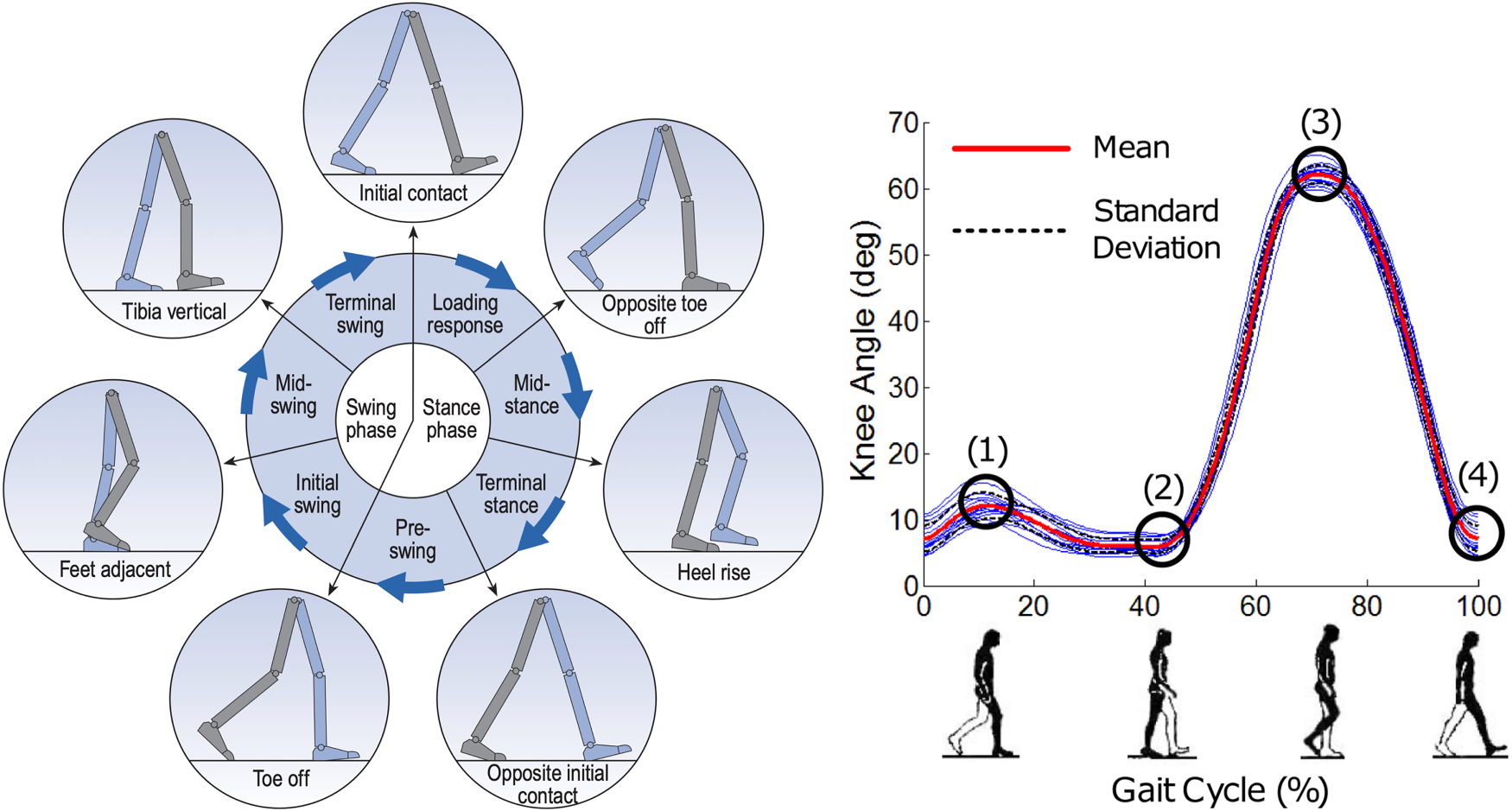
Gait cycle and knee angle. Left image from Whittle (2014). The left image’s gait cycle is based on the right leg (grey). Right image from Ahn and Hogan (2012).
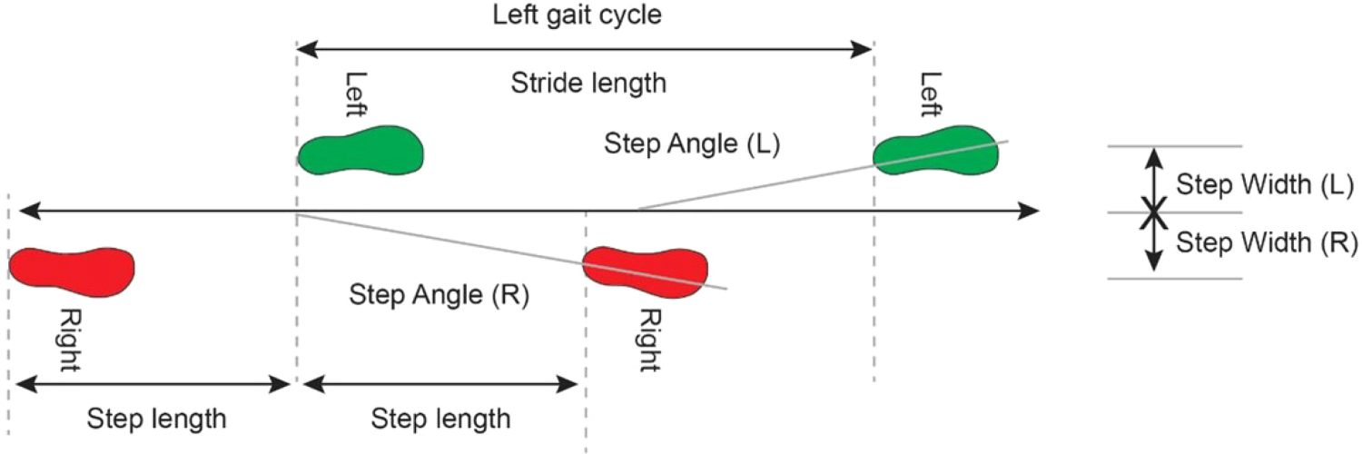
Stride and step in human gait. Image from Tekscan (2019).
The lower limbs are crucial in automatically detecting the phases in gait. Accordingly, they must be accurately determined if the gait phase and, consecutively, the stride length and step length are to be estimated correctly. Figure 1 shows the lower limb movements during gait.
We recorded our own dataset, as none of the existing datasets fit our needs perfectly. The dataset was recorded at the EASE BASE (Meier et al., 2018) using the Optitrack Motion Capture and Intel RealSense D435 depth sensor. It was recorded from one person walking freely in the room and comprised 89 min of data. It contains 157,825 frames over six sessions of 14:50 min each at 120 GB total. Of the samples, 1.50% of depth frames and 2.95% of the motion capture joints were lost to technical issues. Figure 3 shows a frame of the recorded single-channel 16-bit depth image with
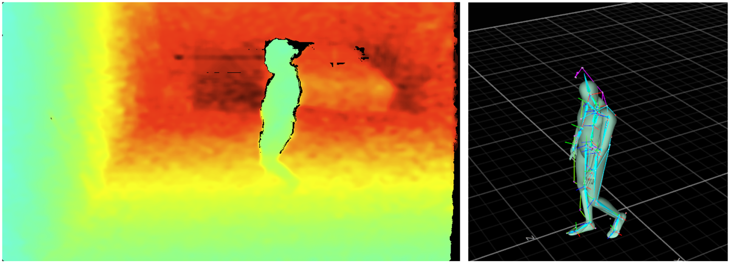
Left: Colorized example image from the depth sensor. Turquoise/green is close at
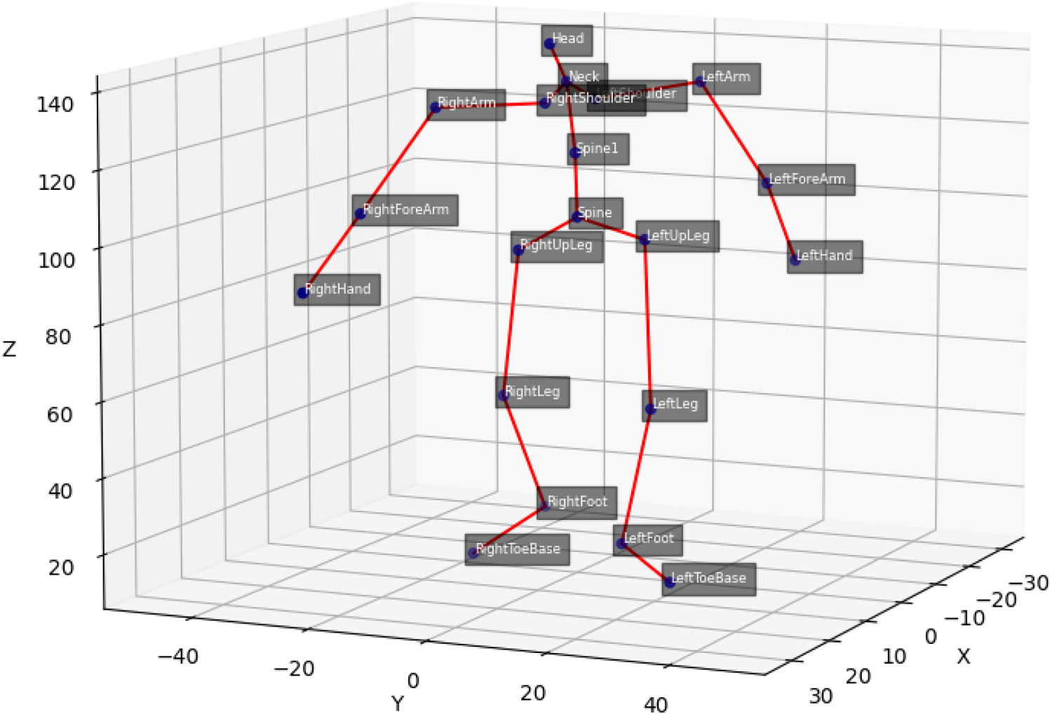
Skeleton joints of the motion capture data.
The motion capture and depth cameras use active infrared emitters that influence each other’s precision when emitting simultaneously. Therefore, the RealSense depth camera was hardware synced with the Optitrack motion capture via an inversed output sync signal from the Motive software via Optitrack eSync 2 and custom input connector
2
to the RealSense.
3
The different voltages are converted to match. The inversed exposure signal has a raising edge once the motion capture emitters are turned off, which triggers the depth emitters and shutter, as shown in Figure 5. In other words, the sensors are synced to record directly after each other so the emitters do not interfere. The RealSense could technically record with 60 fps at 848
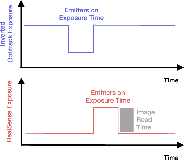
Exposure signals. The rising edge in the Optitrack exposure signal triggers a RealSense frame. Image inspired by github.com/IntelRealSense/librealsense/issues/10926 (last opened: 26-10-23).
Incomplete motion capture and missing depth frames pose challenges in machine learning. Removing incomplete or missing frames from a sequence leads to inconsistent timings, which are relevant to sequence models, specifically if multiple consecutive frames are missing. Alternatively, interpolating incomplete and missing data leads to subpar data quality. Therefore, we decided not to interpolate missing depth frames. Additionally, we evaluate both linearly interpolated and removed incomplete motion capture frames.
As stated above, the main setup objective was for the subject to move freely, which they did. On some occasions, they left the field-of-view of the depth camera but remained within the motion capture recordings. While unintended, this poses a great challenge, as it lets us simulate incomplete coverage, which will always happen in the real world and should be addressed using sequence models, specifically if the participant leaves and enters the field-of-view for only a short period.
The evaluations of all methods and their respective chapters are shown in Figure 6. The two data sources are depth frames and hardware-synced motion capture. The human pose estimation is the first evaluation in Section 3. It compares the estimated joint positions to the recorded motion capture frames. Section 4 then compares the stride length calculated from the pose estimation to the estimated and manually verified stride-length estimation based on the motion capture. Since the participant is to move freely in the laboratory, the ground truth stride lengths cannot be predetermined. They would have to be recorded alongside sensors like gait carpets or (semi-) manually annotated based on the observed depth video. We opted for the latter, which automatically estimates the stride length from the motion capture data and verifies it manually based on the depth video.
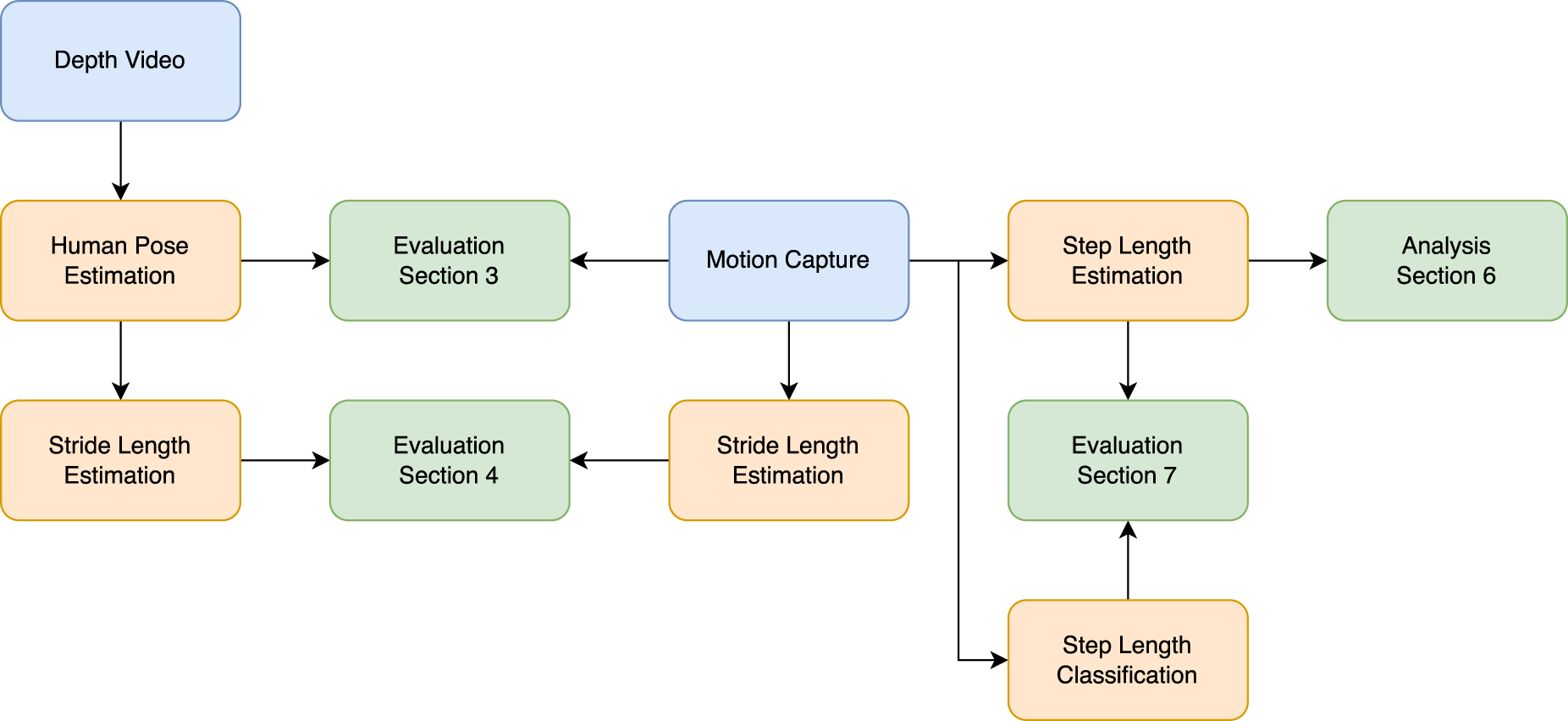
Evaluation methodology. Blue: data source, orange: algorithm, and green: evaluation.
The stride-length estimation already showed quite some variability, which is why we opted to initially evaluate the step length estimations and classifications on the motion capture and later transfer this to the estimated human poses (see Sections 5 to 7). The step length estimation compares different estimation methods, including using foot joint distances (de Queiroz Burle et al., 2020) and an approach using center of mass (Dubois and Charpillet, 2014a). Similar to the stride-length estimation, the ground truth for the step length classification is semi-manually annotated utilizing the compared step estimations and manually checking for correctness.
The train, test, and validation splits differ slightly per evaluation, but most use session six as the test set. For the human pose estimation, we used session six as a test set (as done by Hartmann et al. 2024). We wanted to check if early stopping would be beneficial over setting fixed numbers of epochs. Therefore, we used a random 90/10 split in the frame based methods and session five in the sequence based model as a validation set (as opposed to no validation set by Hartmann et al. 2024). As shown in Section 3.3, this would not have been necessary. The stride-length estimation does not require any parameters to be learned. However, since it is evaluated with the output from the pose estimation, it is only assessed in session six, as the pose estimation would have seen the other five sessions during the training. The step length estimation does not require validation nor a test set, as these algorithms do not need any parameters to be learned. Conversely, no clear ground truth exists for these algorithms as different algorithms can be claimed to be the gold standard. In Section 6, we compare each of their outputs. The step length classification is evaluated using windows of the motion capture data. The set of windows is split into 80% training and 20% test set in a five-fold cross-validation, as no session dependencies need to be considered here, and each model training time is low enough to afford this.
Closely following our previous work (Hartmann et al., 2024), in each step and depending on the task, different metrics are used. Several metrics include a variation for which a lower value is better. These variations are only used for plotting as they loose some information. For example, the metric stride percent (SP) gives the ratio of strides detected versus actual progress on percent. The best value is 100%, where lower indicates little recognized strides, and higher indicates too many strides. Its variation denoted
Human pose estimation
The human pose estimation relies on four metrics to measure how well each joint is predicted from the video input. Three focus on the joint location, while the fourth considers the skeleton created from these joints.
The

The

The stride-length estimation utilizes four metrics as well. We assess the amount, length, distribution, and total distance.


The step-length classification evaluation relies on accuracy as the primary metric and confusion matrices for further interpretation.
The accuracy denotes the number of correct classifications over the number of samples. Higher is better, with a range of 0%–100%.

A good indicator for skeletal precision is the MBSD, as described in Section 2.5. The MBSD in our dataset for all motion capture bones is 0.578 cm, with the left upper arm being most stable at
The optimum range for the D435 is 30 cm–3 m, according to Intel.
4
The RMS depth error is
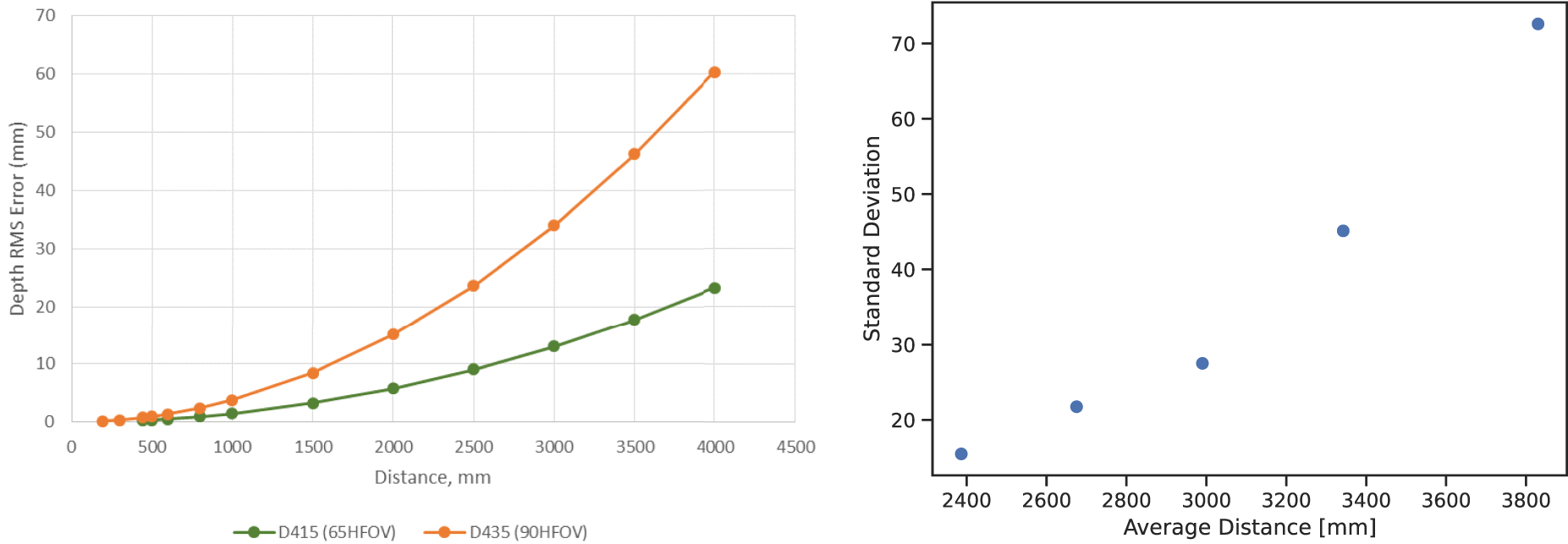
RealSense root mean square (RMS) and standard deviation over recorded frames without participants at different depths. Left image from Grunnet-Jepsen et al. (2020).
The human pose estimation task is given a (sequence of) depth frames with or without a person in the frame and predicts the according motion capture data. It is the building block for most subsequent tasks, and its errors propagate to the subsequent stride-length estimation.
We considered two approaches: frame based and sequence based pose estimation. The former predicts the bones based on a single depth image, while the latter utilizes multiple context frames to indicate the last motion capture frame. Frame based approaches have shown outstanding performances while being the less complex model. However, time context can smooth the predicted marker positions and thus create a more stable result.
Frame based
Similar to Hartmann et al. (2024), four convolutional neural network (CNN) architectures were evaluated. However, as discussed in Section 2.4, the data split was changed to include validation data to allow for clean early stopping. All data loaders shuffled the training data, and all models were trained using the L1 and MSE loss functions. Furthermore, all models were trained with interpolated as well as removed incomplete motion capture frames and evaluated on both test sets (all frames and only those where the participant is evident in the depth image).
The baseline CNN architecture consists of three convolutional layers with Max-Pooling and RELU-activation, as shown in Figure 8. The output size is 63, that is, the three dimensions of all 21 markers. The 164 million parameters are trained using the Adam optimizer, a learning rate scheduler, and early stopping based on the validation loss or a maximum of 100 epochs, whichever applies first.
Baseline convolutional neural network (CNN) architecture. Image from Hartmann et al. (2024). This publication’s output is 63 (instead of 126, with rotation data).
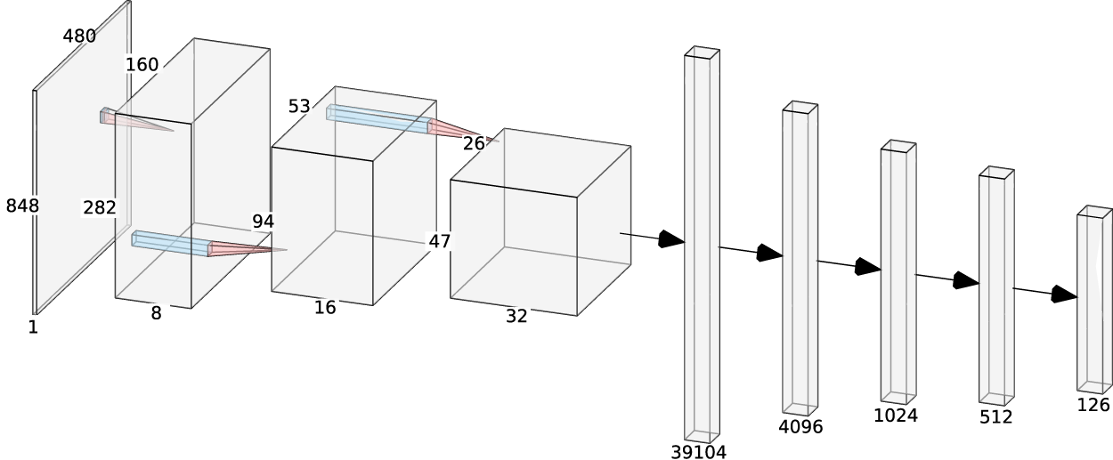
The second architecture is based on the Li and Chan’s work (Li and Chan, 2015) and uses a fourth convolutional layer and a dropout layer with a 25% dropout. The architecture is shown in Figure 9. The dimensions were adjusted from the Li and Chan’s RGB input to our single channel depth input. Like the baseline CNN architecture, the Adam optimizer was used for training. A variation of this model includes using an average pooling layer in the first layer to reduce the number of trainable parameters from 106 to 13 million. Like the baseline CNN, this model is trained using the Adam optimizer, a learning rate scheduler, and early stopping based on the validation loss or a maximum of 100 epochs, whichever applies first.
Li and Chan based convolutional neural network (CNN) architecture. Image from Hartmann et al. (2024). This publication’s output is 63 (instead of 126).
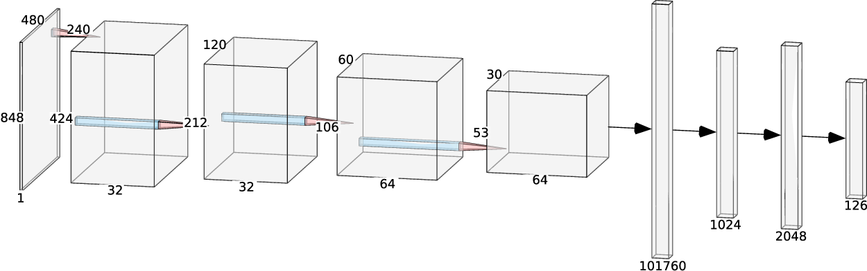
The third model is based on the ResNet50 architecture used by Sun et al. (2017), as shown in Figure 10. The SGD optimizer was used with a momentum of 0.9, a learning rate of 0.03, and a weight decay of 0.0002.
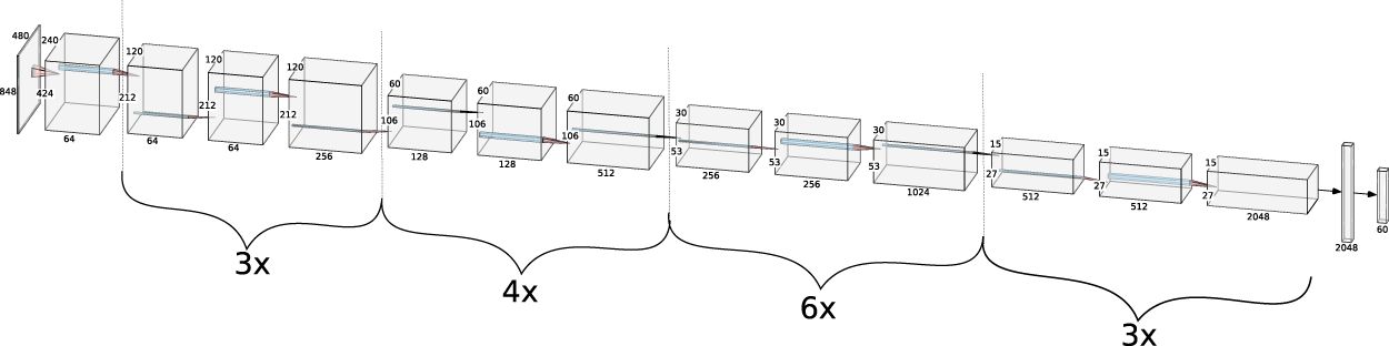
ResNet50 architecture. Image from Hartmann et al. (2024). This publication’s output is 63 (instead of 126).
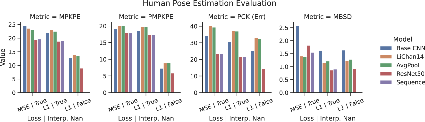
Table 1 shows the results of all frame based model evaluations. The best value in each metric is marked in bold. Figure 11 also gives a quick overview of model comparisons. Both show that models trained and tested on interpolated incomplete motion capture frames perform considerably worse than those without interpolations. Similarly, the performance is better when tested only on the RealSense frames a person is visible in. According to Hartmann et al. (2024), ResNet50 performs best, but all models are pretty close. Note that due to the introduction of a validation set, the performance of all models compared to Hartmann et al. (2024) is consistently slightly lower. The models trained with the L1 loss function generally perform better.
Human pose estimation results across models (testset = all).
Frame based pose estimation results.
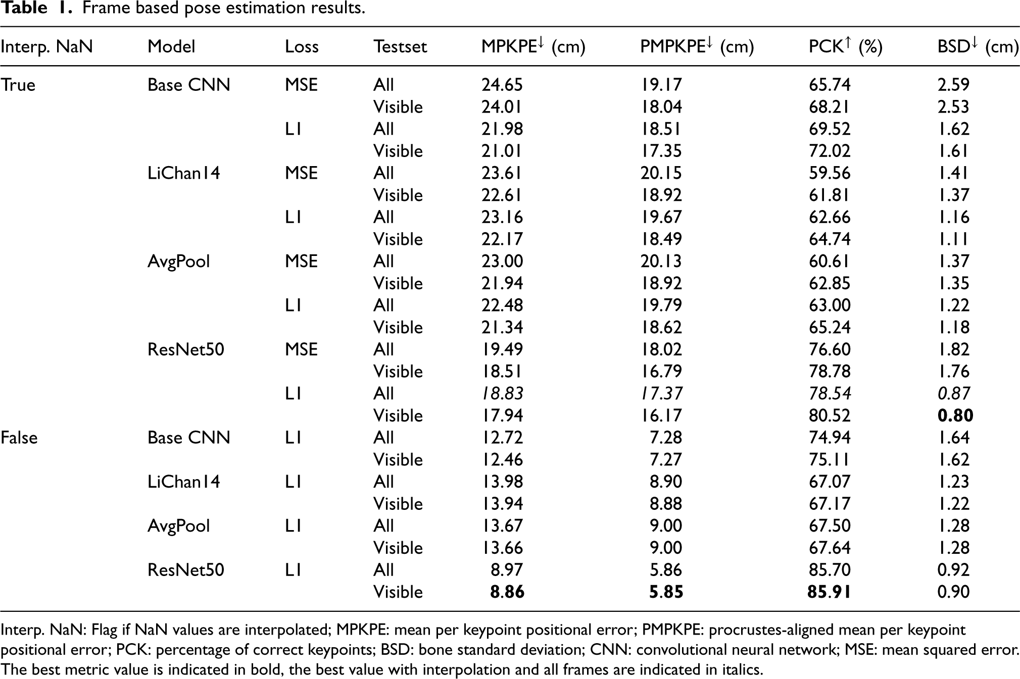
Interp. NaN: Flag if NaN values are interpolated; MPKPE: mean per keypoint positional error; PMPKPE: procrustes-aligned mean per keypoint positional error; PCK: percentage of correct keypoints; BSD: bone standard deviation; CNN: convolutional neural network; MSE: mean squared error.
The best metric value is indicated in bold, the best value with interpolation and all frames are indicated in italics.
The sequence based model of choice is the ResNet50 architecture, as it performed best in the previous frame based iteration with an added LSTM and fully connected layer. It gets a context of 15 frames as input and predicts the last frames’ motion capture markers. The aim is to improve smoothness over time and accuracy over frames where the person is not in the depth field-of-view. The models were first trained separately, combined, and re-trained for a single epoch. The LSTM training on the ResNet50 extracted frames used the Adam optimizer, a learning rate scheduler, and early stopping based on the validation loss or a maximum of 300 epochs, whichever applies first.
Table 2 lists evaluations with MSE and L1 loss functions. Similar to the frame based approaches, the L1 loss models perform slightly better.
Sequence based pose estimation results.
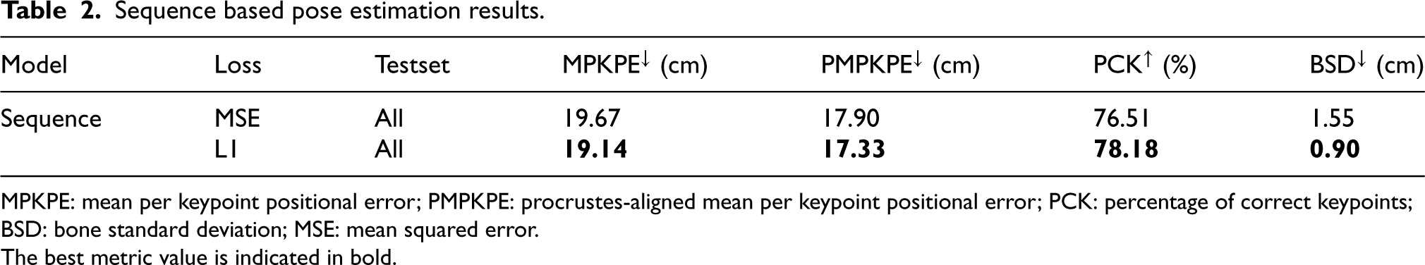
Sequence based pose estimation results.
MPKPE: mean per keypoint positional error; PMPKPE: procrustes-aligned mean per keypoint positional error; PCK: percentage of correct keypoints; BSD: bone standard deviation; MSE: mean squared error.
The best metric value is indicated in bold.
Figure 11 shows the plotted summary of all models. Note that the PCK is plotted in its PCK(Err) version, where lower is better. Note that the sequence model was not trained and tested without the interpolated motion capture frames, as the length of missing frames would be too considerable for proper time modeling. As discussed above, the best performance is achieved by skipping incomplete motion capture frames in training and testing across models. The Sequence model performs slightly worse than the ResNet50 on its own. However, remember that the train/val/test split between the frame based and sequence based models differs to avoid information leakage into the validation set. If trained with the L1 loss, the Baseline CNN outperforms the LiChan model variations in all but the MBSD metric. The AvgPool variant performs on par with the LiChan model and is often slightly better while using significantly fewer parameters. However, considering the loss curves in Figure 12, most models could learn more if provided more time and data, which could reverse the previous observation. Furthermore, the loss curves show that the early stopping would not have been necessary for these training runs, with all of them reaching the maximum of 100 epochs and continuously showing slight improvements. With this amount of data, the validation test could have been omitted.
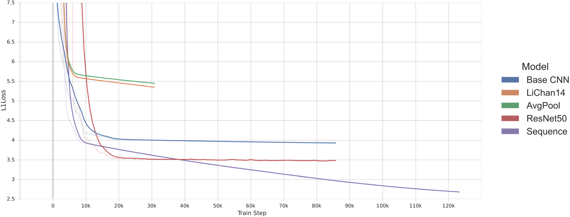
Human pose estimation loss curves.
As discussed earlier, direct comparison to SotA is difficult, as the aforementioned NTU RGB+D dataset is used primarily for human activity recognition. Most of the highly accurate pose estimation works on (manually annotated) RGB images, like the paper by Chun et al. achieving an MPKPE of 15.6 mm (Chun et al., 2023) on the Human3.6 M dataset (Ionescu et al., 2013) by fusing multiple cameras of the dataset in a deep learning approach. While 15.6 mm is incredibly accurate, the settings of multiple calibrated RGB cameras, as opposed to a single depth camera, are drastic and make a direct comparison difficult.
The stride length task estimates the distance between the same foot joint in two consecutive strides based on the depth image based human pose estimation. As described in Section 2, the prediction and ground truth are calculated with the same algorithm but slightly different hyperparameters.
Stride length algorithm
The core idea is based on the not-moving foot during ground contact in the stance phase (Perry and Burnfield, 2010; Whittle, 2014). The speed is calculated using the Euclidean distance between two consecutive depth frames/motion capture frames. The variability, specifically in the depth frames, is counterbalanced using a second-order Butterworth filter with a cut-off at 4 Hz.
Figure 13 shows the speed of the left foot over a 13-second window. As can be seen, the speed regularly is zero, indicating a mid-stance. The algorithm detects all local minimums and enforces a distance hyperparameter that ensures a minimum number of frames between two minima/mid-stances to prevent noise from influencing the results.
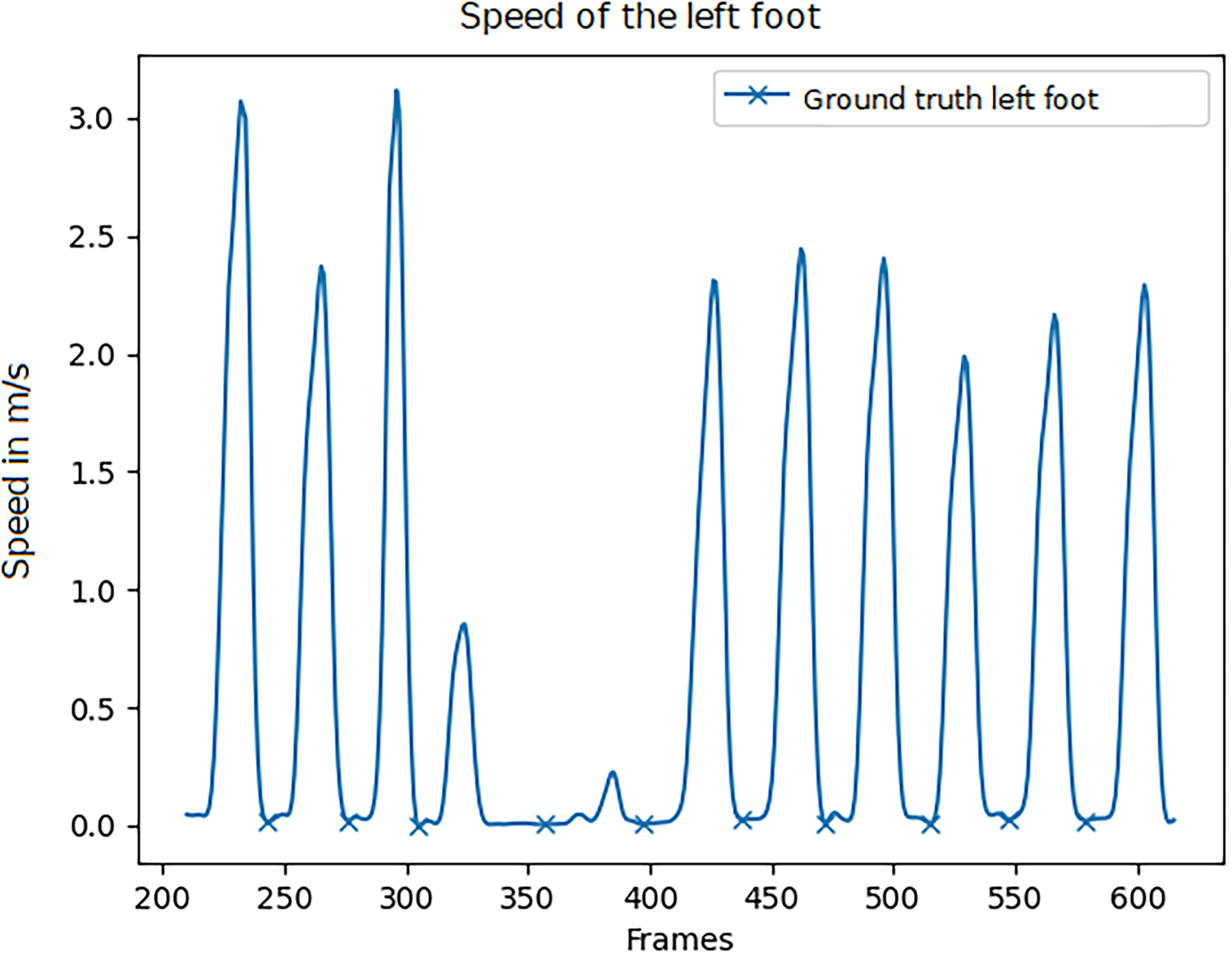
Speed of the left foot. Detected middle stance phase marked with X. The image shows 13 s.
The subject was able to move freely in the room. Thus, the ground truth stride lengths cannot be predetermined or marked on the floor and must be estimated from the motion capture, as discussed in Section 2. The minimum-distance hyperparameter was tuned by hand to 20 frames for the ground truth data, such that the number of strides matches the ones taken during the session, as manually determined and checked. The stride lengths for this dataset are calculated using the motion capture marker positions of the foot joints at their low point in acceleration, that is, when placed on the ground during the single support of the stance phase, see Section 2.1. The average stride length and variation of the single recorded individual can be seen in the later Figure 16. The average stride length is 38 cm.
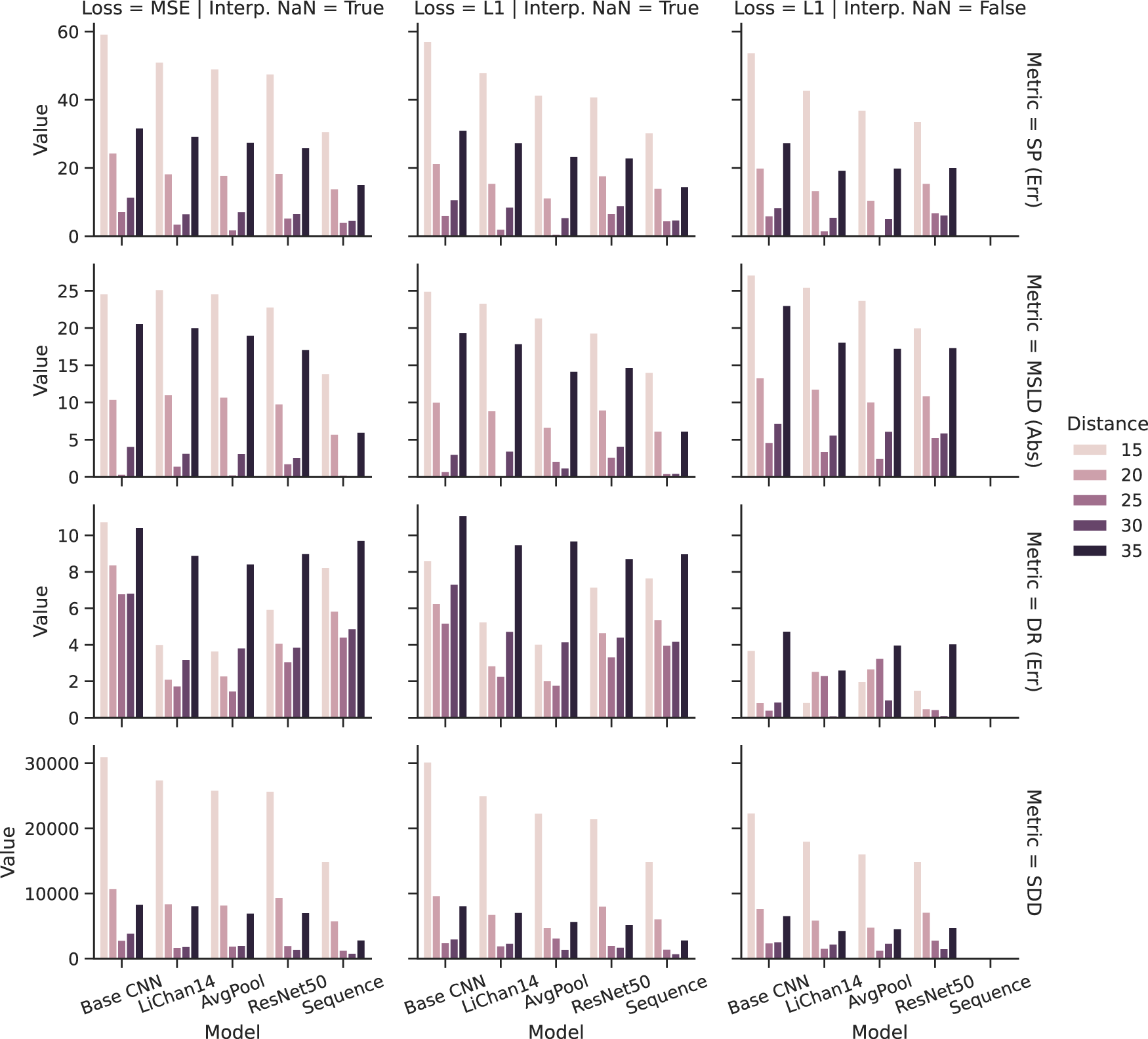
Stride estimation evaluation over models, distance hyperparameter, loss function, not a number (NaN) treatment, and metric.
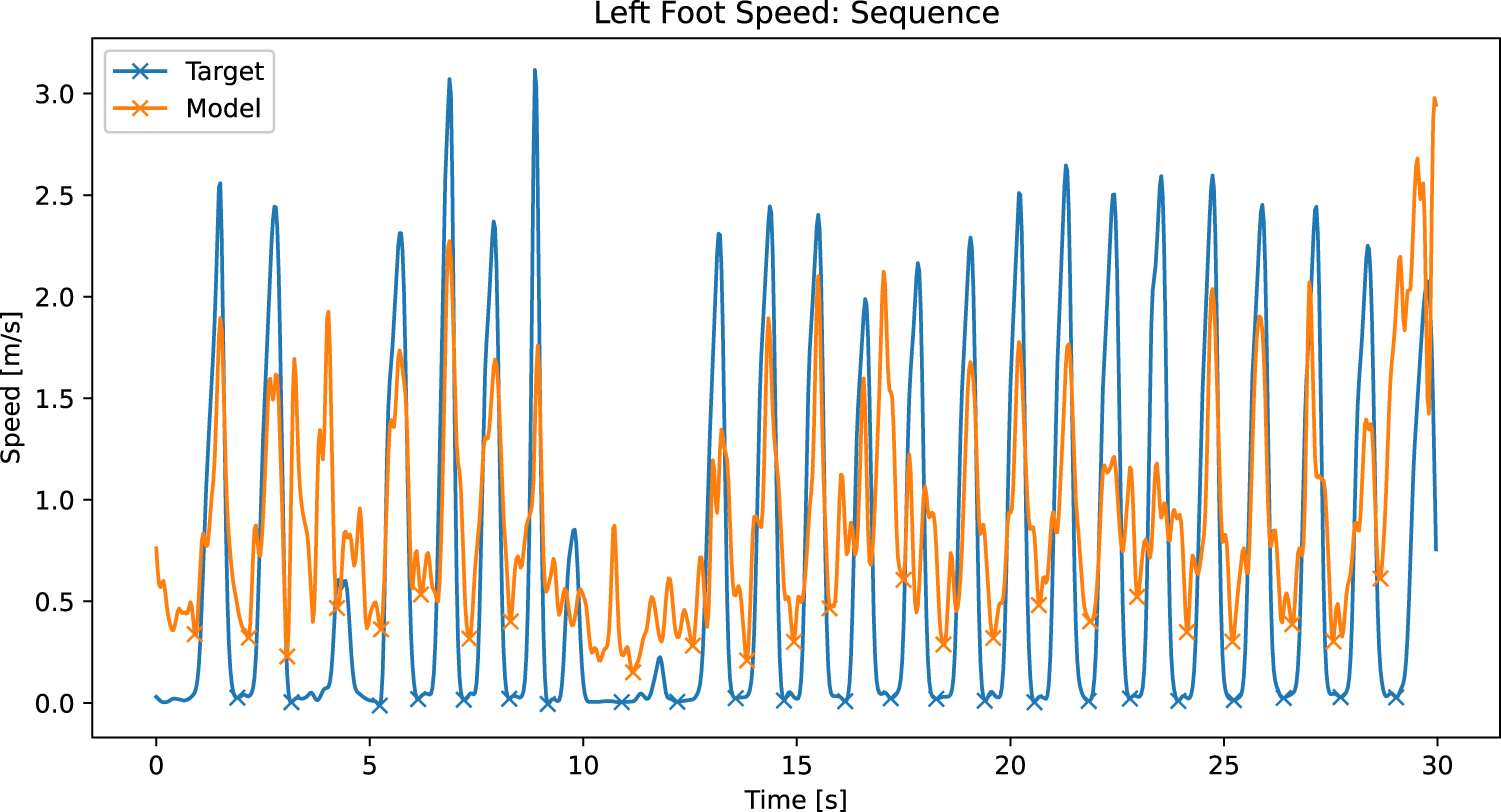
Speed of the left foot as recorded with the motion capture and calculated from the sequence based human pose estimation. Xs mark the detected mid-stance phases.
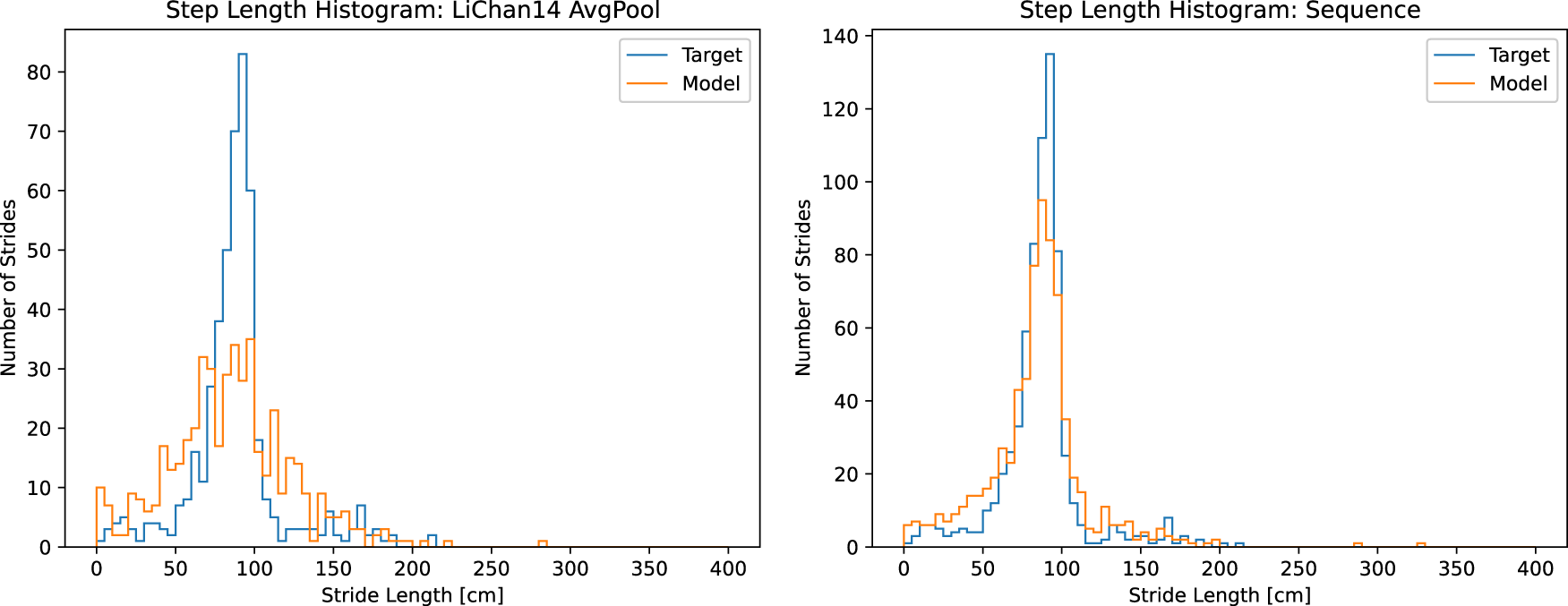
The 5 cm binned stride-length histograms. Left as predicted by the LiChan14 AvgPool model and right as predicted by the sequence model. The y-axis uses different scales, as the left is without interpolating the incomplete motion capture frames, and the right is with interpolation. The shapes remain comparable.
The stride-length estimation algorithm is the same as that applied to each pose estimation model. However, the results might differ depending on the foot joint accuracy. Figure 14 shows the stride-length estimation results in more detail, also depicting the different results for different minimum distance values. Note the slightly different metrics instead of Table 3. In this figure, lower is always better. The figure shows the best possible performance with this algorithm, depending on the chosen distance hyperparameter, which is not the same as the train/test split. For the latter, please refer to Hartmann et al. (2024). A distance of 20–30 frames marks the best choice for the stride-length estimation task, as indicated by the lowest scores in most metric and model combinations. Most notably, all models perform best in the distance ratio metric if the incomplete motion capture markers are omitted.
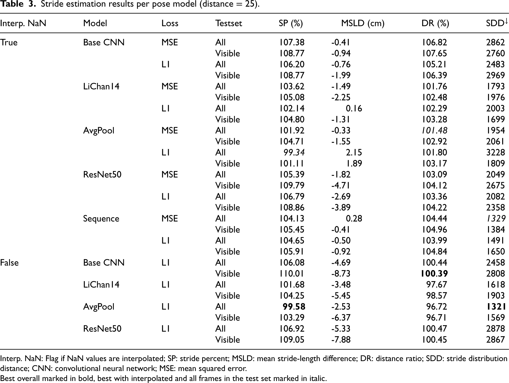
Stride estimation results per pose model (distance = 25).
Stride estimation results per pose model (distance = 25).
Interp. NaN: Flag if NaN values are interpolated; SP: stride percent; MSLD: mean stride-length difference; DR: distance ratio; SDD: stride distribution distance; CNN: convolutional neural network; MSE: mean squared error.
Best overall marked in bold, best with interpolated and all frames in the test set marked in italic.
Table 3 shows the model’s performance for the best-performing distance hyperparameter at a minimum of 25 frames in more detail. The results show different models providing adequate inputs to the stride-length estimation, resulting in mixed results in each metric. The average pool variation of the LiChan14 model performs best if incomplete motion capture frames are omitted in the train/test sets about the stride percent metric with 99.58%, indicating it almost perfectly detects all made strides. The lowest stride deviation histogram distance score further supports this. However, this model underestimates the average stride length by 2.53 cm, underestimating the total distance moved. Considering the mean stride-length deviation, the LiChan14 model performs best, closely followed by the average pool variation on average overestimating the stride length by 0.16 cm but overestimating the number of strides taken and, therefore, overestimating the total traveled distance. Interestingly, the baseline performs best in the total traveled distance, even though it heavily overestimates the number of strides taken. Notably, the ResNet50 model, which outperformed in the pose estimation task, does not keep that result in the stride-length estimation task. It follows the base CNN closely in the distance ratio metric with just a 0.06% difference.
If only considering the interpolated frames with all frames in the test set as reported by Hartmann et al. (2024), the picture is a little clearer, with the LiChan14 variations generally performing best, except in the stride histogram distance. The best stride percent model is the average pool LIChan14 variation (99.34%). The original LiChan14 still performs best in the MSLD (0.16 cm). The best DR model is again the AvgPool variation (101.48%), while the sequence model performs best in the SDD metric (1329).
Figure 15 shows the left foot’s speed, the recorded motion capture, and the sequence model predictions. As shown and discussed earlier, the speed in the ground truth regularly drops to zero during the stance phase. The sequence model predictions are less stable but show the same overall pattern, missing the peak highs and lows.
Figure 16 shows the stride-length histograms for the LiChan14 AvgPool variation and the sequence model. The y-axis uses different scales, as the left is without interpolating the incomplete motion capture frames, and the right is with interpolation, leading to different total amounts of strides. Both models the ground truth shape well, but the Sequence model better models the high-density area between 50 and 100 cm stride length. Less often getting the strides precisely right, as indicated by the worse MSLD score (see Table 3), but better estimating the total amount of steps taken (see SP in Table 3).
Figure 17 shows the detected strides in the first 30 s analogous to the plot of the foot speed 15. The feet are colored (left foot blue and right foot orange), and the ground truth is depicted in a lighter color; the prediction is opaque. The subject starts walking to the left, then does a 180-degree turn by doing a backward step on stride three, then proceeds to walk forward in a circle counterclockwise and then another clockwise. Note that stride 3 corresponds to the third marked target stride in Figure 15, explaining the low speed between the first and second stride. The predicted left foot in the center corresponds to the first detected stride in the speed plot. Figure 16 shows that most predictions are close to the ground truth and often slightly shifted specifically with further distance to the sensor. Note that everything beyond
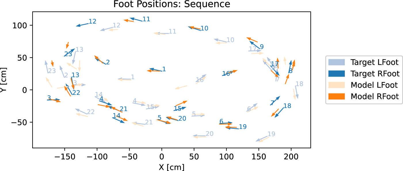
Detected strides in the first 30 s of session 6. Ground truth in orange, prediction in blue. The left foot is opaque, and the right foot is slightly transparent. The number indicates the detected stride number.
Visual inspection and the overlayed speed plot Figure 15 indicate that the extremities and specifically the foot joints are less stable over time in the estimated human pose compared to the motion capture frames. They are making the actual foot speed harder to estimate and, thus, the stride-length estimation less reliable, resulting in mixed results. According to Hartmann et al. (2024), the stride-length estimation results are similarly distributed, with the LiChan14 scoring best in the stride percent and mean stride-length deviation metric. However, the ResNet performs best in the total distance traveled and the stride deviation histogram distance. In neither case does baseline CNN perform best.
An area for improvement in the stride-length estimation is the current focus on the foot joints. While using only the foot joints suffices for ground truth calculation where the motion capture joints are very stable, the stride estimation needs to be more robust to occlusions and less stable model joint predictions. One important performance factor here is the inclusion of further joints, as we will discuss and evaluate in Section 7. We conclude that stride-length estimation is very promising and could create very good results, despite session six being one of the most challenging sessions regarding incomplete motion capture data.
Step length estimation
The step length is eminent in gait analysis and while performing various mobility assessment tests such as SPPB (short physical performance battery) (Guralnik, 1994) where it can be utilized for the score calculations. The mobility assessment tests are performed to understand and evaluate the mobility, balance, and fall risk for older adults. Older adults perform different tests, and scores are given, for instance, according to the completion time or if the test is successfully performed. Steps could also be used to determine other gait parameters, such as cadence, which is the number of steps per minute.
The motion capture dataset collected along with the depth camera is used for the step length estimation (see Section 2.4). Figure 4 in the dataset section shows the joints used in the motion capture data. For the step length estimation, the joint’s spine, right, and left foot are the most important. We consider two main approaches to determine the step length. The first utilizes the foot joints, while the second relies on the center of mass.
Foot joint distance approach
The foot joint distance based approach follows de Queiroz Burle et al. (2020) and has three main steps. First, the Euclidean distance between the x and y-coordinates of the left foot and the right foot for every frame in the entire dataset is calculated, and at every peak of the Euclidean distance, a step is detected. The Euclidean distance between the right and left foot for 200 frames and the corresponding step detected is shown in Figure 18.

Euclidean distance between right and left foot and the detected steps at each peak for 200 frames.
For the further calculation of step length from the Euclidean distance between the right and left foot, the vector of the walking direction has to be determined. This vector is used to understand the direction the person is moving so that we can transform the distance between the two feet relative to this vector. The walking direction identifies if the person is walking frontwards, backward, or sideways. This information is relevant in further calculations. The walking direction vector is estimated with the current and last five consecutive frames. It performs a curve fit independently using a linear function on the position of each foot joint. Then, the average of these two curves is taken to get the body’s center.
The frames where steps were taken must be identified. This is distinguished by identifying local maxima in the previously calculated Euclidean distance between the left and right foot joints. These peaks likely correspond to moments when one foot is in front and the other is in back before moving in the opposite direction, suggesting a step. A point is considered a local maximum if it is greater than the two neighboring points. For finding the local maxima scipy.signal.argrelextrema (Virtanen et al., 2020) was used, with an order of eight, that is, the function considers eight points to each side.
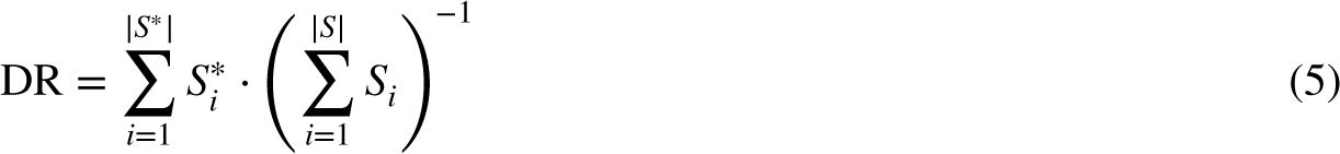
Finally, for the calculations of step length, the spine, right foot, and left foot joints are required. Two vectors are created from the spine to the right and left foot joints. For the exact horizontal distance between the right and left foot, the vectors from the spine to the right and left are projected to the walking direction vector calculated previously. When a step is taken, the spine joint is considered between the right and left foot joints. Hence, the step length is the sum of the vectors from the right and left foot joint to the spine joint projected onto the walking direction vector. Figure 19 shows the projected vectors (P1 and P2) from the right (RF) and left foot (LF) from the spine (S) relative to the walking direction (wd), the vectors
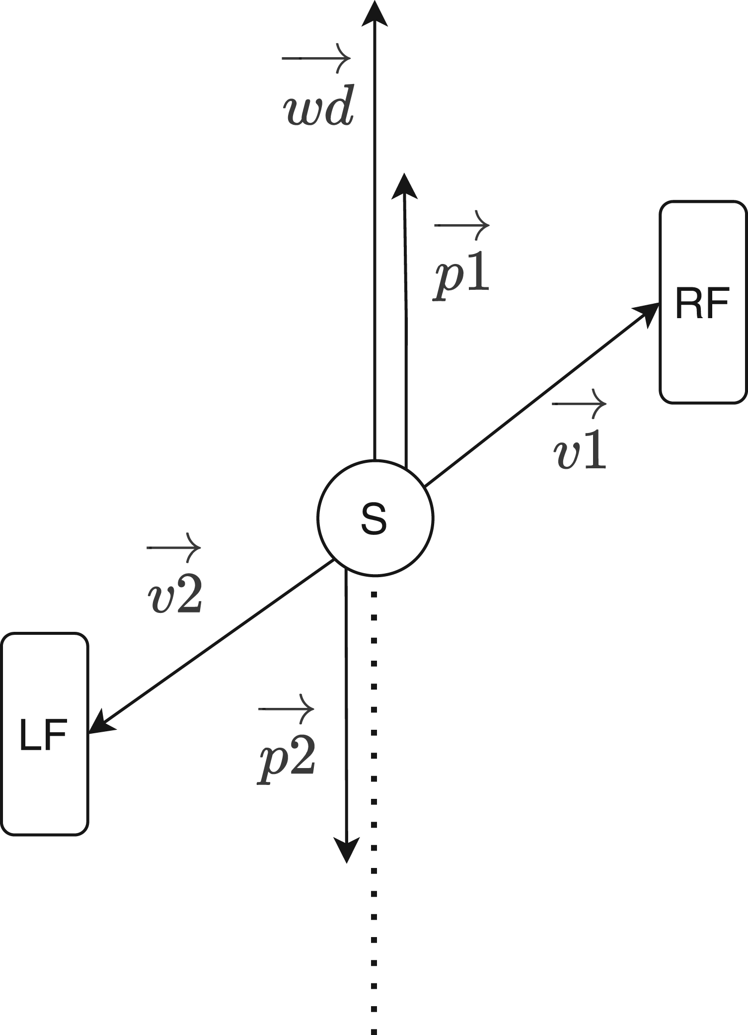
Step length estimation from foot joints and spine joint. Image inspired by de Queiroz Burle et al. (2020).
We used another approach to estimate step length from the skeleton’s center of mass (CoM) (Dubois and Charpillet, 2014b). According to Dubois and Charpillet (2014b), the CoM of the participant’s silhouette is used. In our approach, we consider the spine joint to be the CoM of the skeleton. Then, the change in vertical CoM distance over the ground during the gait cycle is utilized to estimate the step length. Figure 20 shows the vertical position of CoM during walking. The peaks in the vertical position of CoM are found using scipy.signal.find_peaks(Virtanen et al., 2020), each peak denotes a step, and then the Euclidean distance between the position of CoM between each adjacent peak is calculated as step length. The plot of the vertical position of CoM for 200 frames and the steps identified are shown in Figure 21.
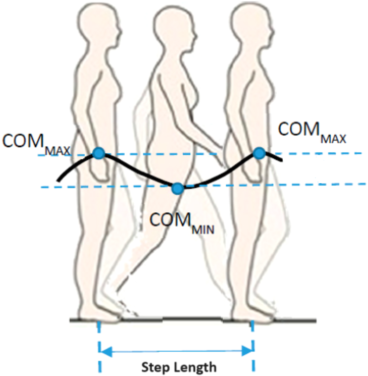
Vertical distance of center of mass (CoM) when walking. Image from Fusca et al. (2018).
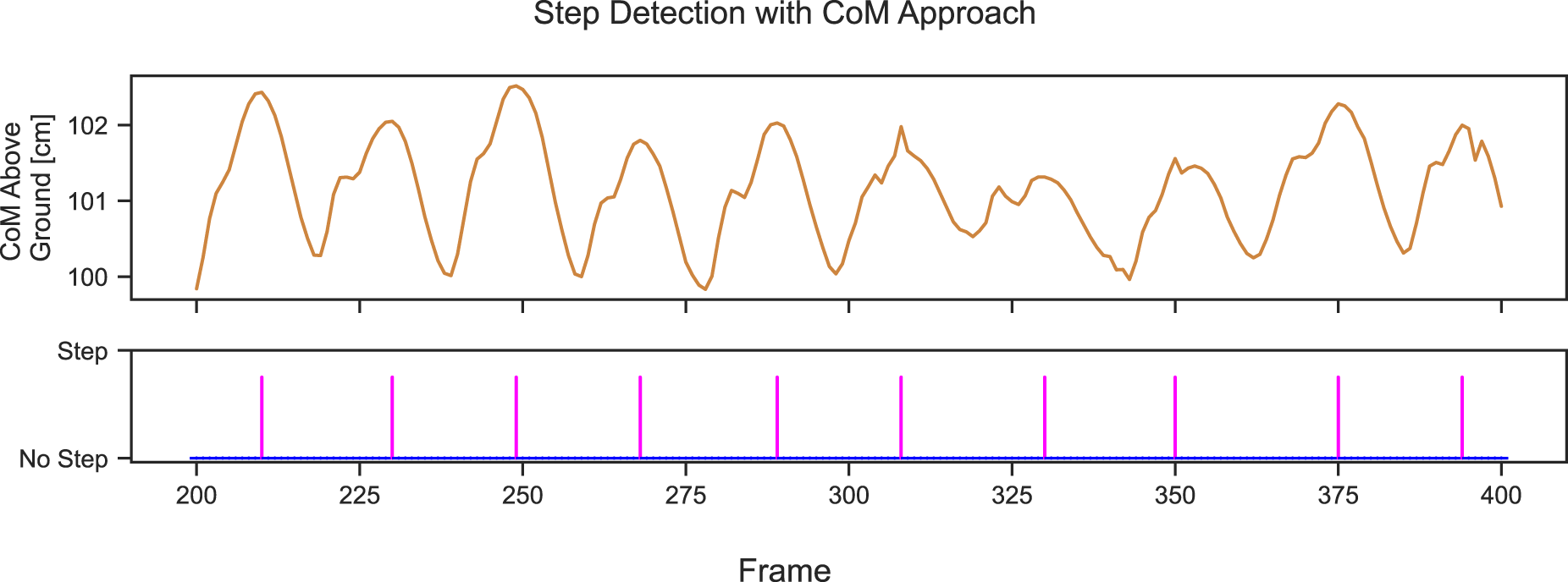
Vertical distance of center of mass (CoM) and the detected steps at each peak for 200 frames.
All of the above approaches, stride-length estimation, foot joint based step length estimation, and CoM based step length estimation, can be compared, as a step is simply half a stride.
Figure 22 shows the steps detected using various approaches. The top plot shows the different signals: the right and left knee angles, right and left foot speed, the vertical distance of CoM to the ground, and the distance between foot joints during the walk. Each knee angle shows a peak during the swing phase and an almost flat angle during the stance phase as seen in Figure 1 Ahn and Hogan (2012); Qiu et al. (2017). The signal interplay is nicely shown. The CoM is highest when the feet are next to each other during the swing phase, which coincides with the lowest distance between both feet and also the highest speed of the foot. The highest knee angle is slightly offset as it occurs during the initial swing phase once the toe leaves the ground. Note that in this figure, each signal is very clean, as the participant is walking normally. Furthermore, each of the calculated signals is based on motion capture rather than the less stable depth based extracted skeleton. The lower plots show the detected stride or step for each method. The motion captures stride, and the depth based stride is the ground truth and model estimation from Section 4. The shown plot uses the L1-trained sequence model for stride estimation. For good measure, we included a segmentation based stride detection approach using the TSSEARCH libraries DTW segmentation method (Folgado et al., 2022) with a hand-selected search query that starts and ends with a right knee angle peak. Note that while this is a simple method, it works well on clean data but might struggle if other actions are performed between strides. Both step detection approaches work as described in Section 5. The plots visualize that a stride consists of two steps, as described earlier, as shown by the double step marks at every stride.
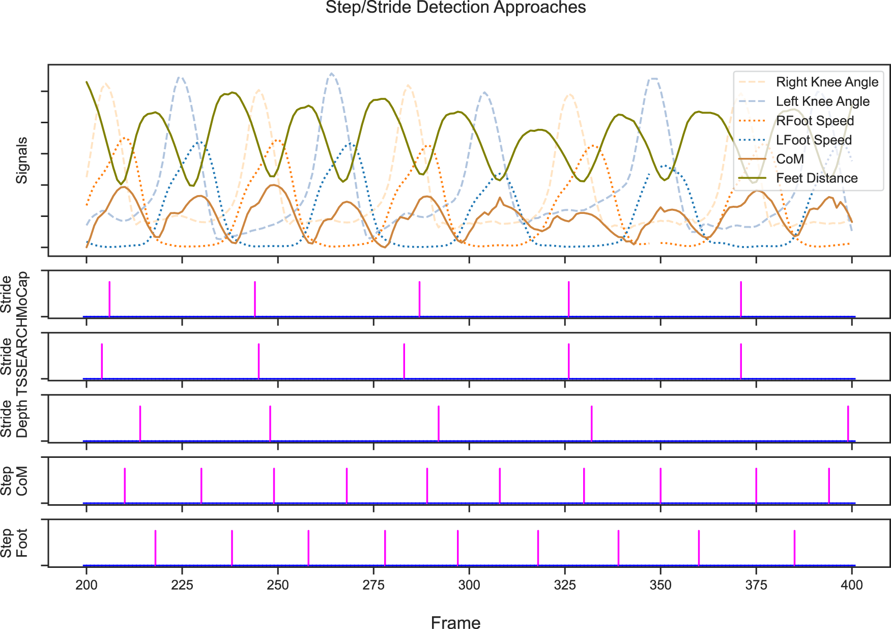
Various approaches of step and stride lengths. The first subplot shows the respective signals used. All signals are re-scaled to fit into the plot. The knee angles and speed share the same scale among each other. Center of mass (CoM) and feet distance do not share a scale with another signal. The lower subplots mark each detected stride/step with a purple vertical line.
The CoM based step detection essentially detects the peak CoM, that is, the adjacent feet during the swing phase or opposing mid stance, while the foot based approach detects the point where the feet are farthest from each other, that is, the lowest CoM or the (opposing) initial contact at the end of a gait cycle. The stride detection on the contrary detects the lowest foot speed, that is, the mid-stance phase or opposing swing phase, and is thus less clear in its exact timing, as the opposing swing phase might take half a second and a single point within that is marked, but quite clear in stride distance, as the measured foot does not move that entire time. These observations are shown in the plot. The steps detected by CoM and foot distance approaches are shifted and interlaced perfectly. The TSSEARCH and motion capture strides are very much synchronized, and the depth based stride detection is slightly shifted from the other stride detection due to a noisier foot speed compared to the motion capture based signals. This noise would also explain the outlier at frame 400, which should be a second (30 frames) earlier.
All of these approaches detect the strides and steps quite well. However, not all of them lead to the same estimated length. As discussed in Section 4, the distance ratio between the motion capture based and depth based stride-length estimation often is not perfect and often over- or underestimates the total distance traveled. Similarly, the step length estimation can vary quite dramatically. Quite often, we are only interested in the change of a person’s step length over time, in which case, the accuracy of the step length itself is less relevant as long as errors are consistent. As done for the stride length, we were interested in quantifying the difference between the two-step length estimation techniques. Calculating the distance ratio between CoM and foot based approaches yields 111.24%, with 578.76 m CoM and 520.26 m foot based estimated total distance in Session One at 1380 CoM and 1396 foot based steps detected each. While the number of steps is pretty close at 16 steps, the total distance with a difference of 58 m is not. Comparing each step to one another is not straightforward, as they do not necessarily detect the same steps. Figure 23 shows the difference between consecutive steps between both approaches in a 5000-frame long subsequence. The difference is mainly within the range of
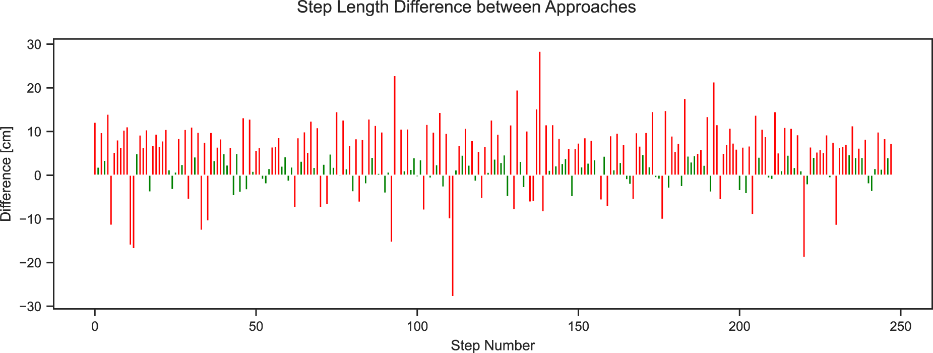
Difference between the two approaches for the calculation of step length for 5000 frames. Differences above 5 cm are marked in red and below 5 cm are in green.
Looking deeper, Figure 24 shows the aligned step lengths in the same 5000 frame subsequence. The alignment is done using the longest matching subsequence of the TSSEARCH library (Folgado et al., 2022), notice the different axes for better signal readability. Similar to the above, the step with an estimated length of 80 cm likely should be detected as two steps instead. Both signals show a distinct pattern, where roughly every six steps a shorter step is detected. This likely is the participant switching direction or walking in a curve. This kind of movement can imply the feet are moving quite far apart while the CoM remains close, thus explaining the difference in detected step lengths and total distance traveled. While this is a probable cause, further analysis should be conducted in future work comparing the different cases each algorithm handles more easily. Nevertheless, we continued with the foot distance based approach for the subsequent step length classification.
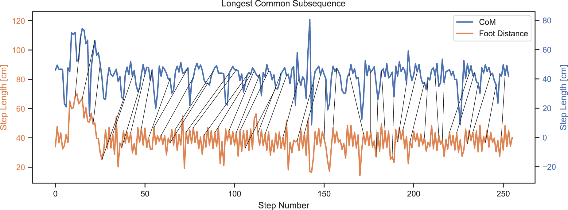
Estimated step lengths based on center of mass (CoM) and foot distance over a 5000 frame subsequence. Alignment based on longest common subsequence.
The step length classification task predicts four different classes (small, normal, big, and no step) from the x, y, and z-coordinates of the motion capture joints. The step length classification is essential while performing various Mobility assessment tests such as SPPB to calculate the score if the foot joints are less accurately detected or the step length itself is less important than its relation to the individual’s normal step length. To make this a classification task, four classes are created based on the calculated step lengths: no step, regular, short, and significant. The normal range is considered according to the age, height, and sex of the participant in the dataset. The minimum step length found was 1.56 cm, mainly referring to changing the direction of walking or turning. The maximum step length found was 91.24 cm; hence, the average step length was 38 cm (i.e. half the stride length depicted in Figure 16). Every step 20% higher than the average length is considered a big step, and every step 20% smaller than the average length is regarded as a small step. The classification of the classes is shown in Table 4. A class for no step is used in the classification process so that the model better understands if a frame is a step in the first place. Table 4 shows the range of step length and each class.
The four target classes based on the average step length.
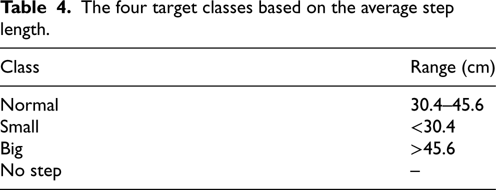
The four target classes based on the average step length.
The entire dataset has 157,825 frames from six collected sessions. As shown in Figure 25, the data is very imbalanced, as a step is usually not finished but underway. Therefore, the data is downsampled to achieve a less imbalanced set, resulting in 8000 no-step frames. For the classification, an 80:20 split is used on the downsampled data.
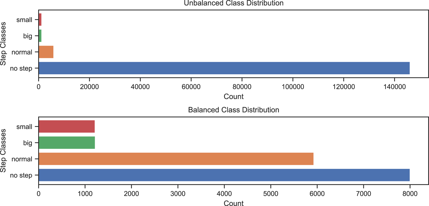
Distribution of step classes in the dataset.
As discussed earlier, not all joints should be equally important to step length classification. With the foot and leg joints being more informative. Therefore, the importance of each skeleton joint in the classification is determined using the feature importance function of the RF classifier. The results are shown in Figure 26. As expected, the most essential features are the leg joints with foot, toe base, up leg, and right and left legs. Accordingly, various experiments were conducted for the classification of step length focusing on the input joints: (1) whole skeleton, where all the joints from head to foot joints are used; (2) using only the right and left leg joints, which includes knee, foot, and toe joints, and (3) all joints except the right and left foot joints (as could happen during occlusion). From Figure 26, we understand that the most important joints are all the leg joints; hence, the best performance is expected in that experiment. Each experiment was analyzed with two approaches: (1) frame based using KNN and RF models and (2) window based using the LSTM model for the classification, extending on Hartmann et al. (2024).
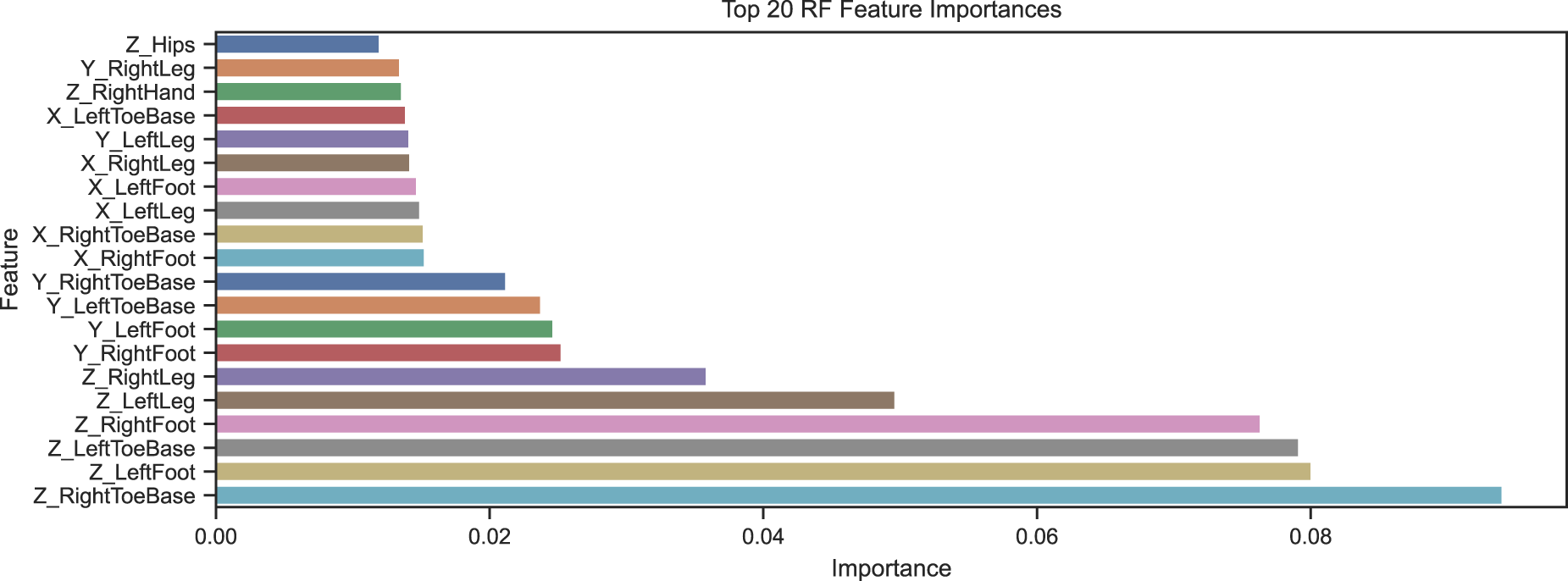
Importance of each joint and their x, y, and z-coordinates in classification of step length.
Here, we used each frame in the dataset and predicted the corresponding step length class. We used two different classifiers, random forest (RF) and K-nearest neighbors (KNN), which showed contrast in the performance of the multi-class classification. A grid search was performed to find the best hyper-parameters of the RF classifier. During the grid search, different combinations of parameters were tried on the samples to reach the best combination that optimizes the classification. After the grid search, the main parameters chosen were the maximum depth of each tree as 20 and the number of estimators as 150. The evaluation of all the approaches used K-fold cross-validation with five folds.
Leg joints only
In this experiment, we used the best-contributing joints: all the leg joints in the skeleton. This framed based approach showed the best accuracy in both RF and KNN. An accuracy of 80% with RF and 77% with KNN was achieved. Figures 27(a) and 28(a) show the confusion matrices of RF and KNN using these leg joints.
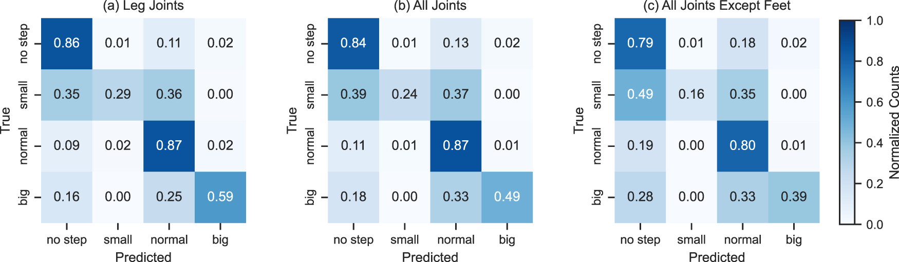
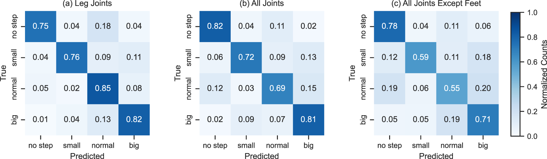
Classification of step length using random forest (RF). Left to right: (a) using leg joints, (b) using all joints, and (c) without foot joints.
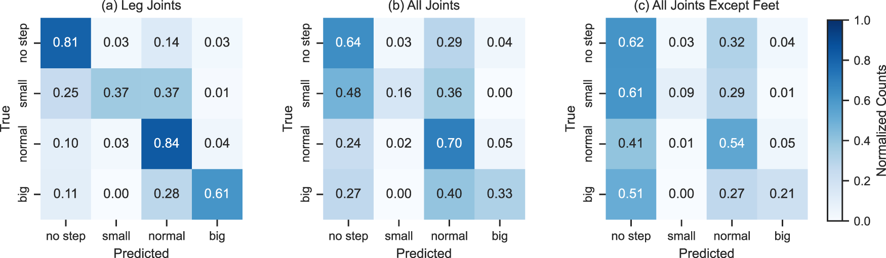
Classification of step length using K-nearest neighbors (KNN). Left to right: (a) using leg joints, (b) using all joints, and (c) without foot joints.
In this experiment, we used all the joints in the skeleton for the classification. This framed-based approach achieved an accuracy of 78% with RF and 60% with KNN, slightly lower than the previous case. Figures 27(b) and 28(b) show the confusion matrices of RF and KNN using all joints.
All except foot joints
In this experiment, we used all joints except the foot joints. This framed based approach achieved an accuracy of 71% with RF and 51% with KNN. As expected, both are worse than in the previous experiments. However, the KNN essentially falls back to the guessing baseline of 48.89%, which refers to the performance a model would achieve that always returns the most frequent class (no step). Figures 27(c) and 28(c) show the confusion matrices of RF and KNN using all except the foot joints.
Context/window-based classification
For the window-based approach, we used an long short-term memory (LSTM) model on a 20-frame sliding window. The model’s input is 20 frames; the output remains the four classes: small, normal, big, and no step.
Leg joints only
In this approach, we used only the leg features in the skeleton for classification. This window-based approach achieved an accuracy of 79%, which is less than the accuracy achieved by the RF model. Still, from Figure 29(a), which shows the confusion matrix of LSTM using leg features, it is clear that even though RF shows better overall performance, LSTM performs better in classifying individual classes.
Classification of step length using long short-term memory (LSTM). Left to right: (a) using leg features, (b) using all features, and (c) without foot features.
In this approach, we used all the joints in the skeleton for the classification. This window-based approach achieved an accuracy of 72%. Figure 29(b) shows the confusion matrix of LSTM using all features. The overall accuracy is also lower than the frame-based approach, but from the confusion matrix, it is noticeable that the individual classification has improved in the window-based approach.
All except foot joints
In this approach, we used joints excluding the foot joints in the skeleton for the classification. This window-based approach achieved an accuracy of 60%. Figure 29(c) shows the confusion matrix of LSTM using features excluding foot joints. The individual classification for each class has improved from frames-based approaches, but overall accuracy is less than the RF-based approach.
Conclusions and future work
In this article, we present our gait parameter estimation from a single depth sensor, a crucial step towards online everyday frailty assessments in elderly care facilities. We collected a 90-minute dataset with custom hardware synchronization of the Optitrack Motion Capture and Intel RealSense D435. Our evaluation involved three deep learning approaches to pose estimation, the application and analysis of algorithms for stride-length and step length estimation based on the CoM and foot distances, as well as three models for the step length classification. We compare the results of all models and tie their predictions back to the signals they are derived from, like the knee angle, foot speed, CoM, or the distance between the feet, and explain their relationships to the gait phases.
The skeleton estimation achieved an 18.83 cm MPKPE in the case of the all-frame test set and NaN value interpolation and 8.86 cm MPKPE in the case of the visible-only test set and removed incomplete frames. In both cases, an error of 2–3 cm can be attributed to the depth sensor and the participant’s distance. We showed that a stride-length estimation algorithm based on this estimated skeleton can achieve a step percent of 99.34% (interpolated NaN), 99.58% (all frames and no interpolation), and distance ratios of 101.48% (interpolated), and 100.39% (non-interpolated). The main future challenge is posed by less clean foot speeds in the estimated human pose as opposed to the motion capture skeleton and, thus, too many small steps being predicted. The sequence model did not improve pure positional accuracy, but led to better step distributions, likely due to cleaner speeds. Overall the skeleton estimation and stride detection worked very well but would benefit from further data, as the omission of the validation set showed improved accuracy. We look forward to applying these approaches to the ETAP and EASE datasets.
The step length estimation using the CoM and foot distance approaches shows both working very well. However, it is hard to measure correctness, even when manually checking results. In session one, the number of steps was miss-estimated by only 16 of
The step length classification showed promising results with 80% accuracy with simple RFs and good recognition across classes with LSTMs. While the feature importance ranking showed the feet joints to be most crucial, using all joints almost performed on par, and using all except the foot joints still performed at 60% with the LSTM, while the KNN falls back to the guessing baseline. Further and more sophisticated approaches with regard to feature engineering, more complex sequence modeling, regression models, further investigations into occlusion, and changes in data with older participants should be investigated.
The next logical step is to combine deep learning-based pose estimation and machine learning-based step length/stride-length estimation into an end-to-end sequence model. This way, both partial occlusions and time context should further improve the stability of all models and can address short out-of-frame subsequences. Another approach currently under investigation is transferring RGB-pre-trained models like AlphaPose, PoseNet, or their architectures into depth only, like done above with the ResNet50 architecture or using similar datasets that focus less on gait (and falls) but have similar modalities like the NTU-RGB+D and the deep Mocap dataset.
A key task remaining is transferring and personalizing to and for older adults and out of laboratory everyday life settings. For this, we recorded 10,000
Overall, we evaluated and demonstrated multiple approaches to estimate the gait parameters based on a single depth sensor, showing very promising and accurate results. The core contributions of this work are the developed pose estimation models and the evaluation of all machine learning models and algorithms, the pipeline and evaluation scheme for every step from depth sequences to stride and step length estimation in a scenario of a freely moving subject, and the in-depth analysis tying the signals, algorithms, models, and gait phases together and highlighting the importance of different joint sets for step length classification. We look forward to integrating these models into real-time scenarios in the ETAP project and studying the intricacies of human gait and movement during everyday activities on the EASE-TSD dataset.
Footnotes
Acknowledgments
The research reported was conducted with these Softwaretools: Numpy Harris et al. (2020), Pandas pandas development team (2020), PyTorch Paszke et al. (2019), Pytorch-Lightning Falcon et al. (2020), Scikit-Learn Pedregosa et al. (2012), Scipy Virtanen et al. (2020), Matplotlib Hunter (2007), Seaborn Waskom (2021), and TSSearch ![]() .
.
Funding
The author(s) received financial support for the research, authorship, and/or publication of this article.
The research reported in this article has been partially supported by the German Research Foundation DFG, as part of Collaborative Research Center (Sonderforschungsbereich) 1320 Project-ID 329551904 “EASE - Everyday Activity Science and Engineering,” University of Bremen (![]() ). The research was conducted in subproject H03 Models of Human Activity from Video and Motion Capture.
). The research was conducted in subproject H03 Models of Human Activity from Video and Motion Capture.
The research reported in this article has been partially supported by the German Ministry of Health (BMG), as part of the Research Project ETAP – Evaluation von teilautomatisierten Pflegeprozessen in der Langzeitpflege am Beispiel von KI-basiertem Bewegungsmonitoring (etap-projekt.de/).
Declaration of conflicting interests
The author(s) declared no potential conflicts of interest with respect to the research, authorship, and/or publication of this article.
Notes
Appendix A. Code
The code for pose and stride estimation can be found here: github.com/Saniamos/smart-cities24. More might be added in the future.