Sage Journals: Discover world-class research

Abstract

Cost effective utilization of renewable biogas requires that the siloxane content be maintained at low parts-per-billion (ppb_v) levels. Infrared (IR) spectrometric methods offer the potential for near-real-time siloxane quantification but are difficult to implement in the presence of certain spectral interferents such as oxygenated volatile organic compounds (VOCs). In this report, a novel two-step gas-stream modification process is implemented in the quantification of siloxanes in biogas by Fourier transform IR spectrometry. The method is demonstrated for synthetic biogas comprising a mixture of methane in nitrogen, with linear (L3) and cyclic (D4) siloxanes present at 100 ppb_v levels, and ethanol, acetone, and acetic acid added as model VOCs at 100 parts-per-million (ppm_v) levels. The first step in the process involves sparging the biogas through water to significantly reduce VOC concentrations. The second step removes residual VOCs and the siloxanes by passage of the gas stream over a low temperature metal oxide catalyst. IR spectra acquired after sparging and after passage over the catalyst serve as near-real-time biogas sample and biogas blank spectra, respectively. The biogas blank spectrum and standard siloxane spectra are next used in a simple least squares reconstruction of the biogas sample spectrum for siloxane quantification. Limits of detection for L3 and D4 are determined to be 9.3 and 6.3 ppb_v, respectively, while limits of quantification are 31 and 21 ppb_v. This method will facilitate the development of simple, inexpensive IR-based devices for on-line and near-real-time monitoring of siloxanes in industrial biogas streams.

Graphical abstract

This is a visual representation of the abstract.

Keywords

Biogas siloxane contamination siloxane quantification spectral interference real-time siloxane detection

Introduction

Biogas is now routinely being produced by anaerobic digestion of liquid and solid organic wastes at municipal landfills and wastewater treatment facilities worldwide.^1–4 Unfortunately, these waste streams frequently incorporate volatile linear and cyclic siloxanes that contaminate the product biogas.^1,4–12 When burned, the siloxanes form silicate deposits on the working surfaces of reciprocating engines and gas turbines, resulting in increased maintenance costs and shortened equipment lifetimes.¹¹ Currently, European standards place a limit of ∼260 parts-per-billion (ppb_v) on volatile silicon in biomethane,¹³ while engine manufacturers often quote somewhat higher values.^3,7,8

Fortunately, volatile siloxanes are easily removed from biogas by passage through activated carbon filters.^8–10^,14,15 However, these filters regularly become saturated and must be replaced.^4,10,16–18 As the siloxane content of raw biogas is often variable,^15,18,19 the time to siloxane breakthrough is difficult to predict.^1,7 Weakly bound siloxanes may also be displaced from the filters by more strongly binding compounds as the composition of the biogas varies in time, leading to unexpected breakthrough events, even prior to filter saturation.^1,9,19 Avoiding potential equipment damage therefore requires near-real-time monitoring and quantification of siloxane content so that all such breakthrough events can be detected and mitigated.

While there is no standard sampling or analysis procedure for biogas,²⁰ gas chromatography–mass spectrometry (GC-MS) provides detailed information on biogas composition and, when properly calibrated, accurate quantification of siloxane content.^1,7 Unfortunately, GC-MS analysis is time consuming, expensive, and cannot be performed in real-time. Samples must first be collected by methods such as solid phase microextraction,^7,21 and then taken off-site for analysis in a testing facility by skilled technicians. Long delays between sample collection and return of the results preclude prompt detection and mitigation of breakthrough events.^{1,7,16,21–24}

Continuous siloxane monitoring in near-real-time could be achieved by simpler, less resource-intensive infrared (IR) spectrometric methods.^17,25 Indeed IR instruments are already available for process monitoring in general,¹⁷ and similar systems could be implemented in the automated monitoring of siloxanes in biogas. IR instruments can be used on-site and seldom need recalibration due to their reliance on the Beer–Lambert Law for quantification.

Unfortunately, the monitoring of siloxanes in biogas by IR spectrometry remains challenging for several reasons. Because the composition of raw biogas streams varies significantly between facilities, and even over short periods of time for individual sources,¹⁹ it may be very difficult or impossible to obtain the method blank required for siloxane quantification. All biogas components other than the siloxanes are present in a method blank. Such a mixture would be very difficult to prepare on-site from pure component gases. Raw biogas also contains components that absorb at or near the same frequencies as the siloxanes.^16,17,25 Importantly, these spectral interferents may be present in much higher concentrations. To date, the difficulties in obtaining a valid method blank and the presence of spectral interferents have precluded the widespread adoption of IR methods for siloxane monitoring.

Spectral interferents of particular concern include methane and carbon dioxide, the main components of biogas, as well as a variety of oxygenated volatile organic compounds (VOCs).^16,17,25 The problems associated with methane and carbon dioxide are readily overcome by acquisition of a valid method blank spectrum and by use of siloxane bands in regions where methane and carbon dioxide are only weakly absorbing. Oxygenated VOCs pose more significant challenges, and their presence may indicate additional problems in the biogas production process. For example, they often appear as a result of inefficient anaerobic digestion of precursor waste. Notably, short chain alcohols and acids that are produced during early acidogenesis steps may not be quantitatively converted to methane when subsequent methanogenesis steps are inefficient.^15,20,26,27 As with siloxanes, many VOCs can be removed by passage of the gas stream through activated carbon, or perhaps over common metal oxide catalysts. Unfortunately, because such methods remove both siloxanes and VOCs, their use in producing a method blank is precluded.

In this manuscript, we report an IR spectrometric method that employs a simple two-step gas stream modification process to first remove oxygenated VOCs by sparging the biogas through water. In the second step, the siloxanes and any remaining VOCs are removed by passage of the stream over a low temperature catalyst. These two distinct gas streams are referred to as the “biogas sample” and “biogas blank”, respectively, throughout this work. Standard siloxane spectra are then employed along with the experimentally obtained sample and blank spectra for siloxane quantification by a simple least squares procedure. This method is demonstrated to yield low ppb_v level detection limits for siloxanes, even in the presence of ppm_v concentrations of oxygenated VOCs. The method is demonstrated for a synthetic biogas mixture comprising methane, nitrogen, and water vapor, with octamethyltrisiloxane (L3) and octamethylcyclotetrasiloxane (D4) as representative siloxanes, and ethanol, acetic acid, and acetone as model spectral interferents. Carbon dioxide is left out of the mixture because it is expected to behave similarly to methane, for which spectral interference is readily overcome by use of a valid blank spectrum. A Fourier transform infrared (FT-IR) instrument optimized for gas analysis is employed in these studies. In the future, this same method could be implemented using simpler IR-based process analysis instruments for automated siloxane quantification in near-real time with industrial biogas streams of unknown composition.

Experimental

Materials and Methods

A compressed gas mixture of 90% nitrogen and 10% methane (90/10 nitrogen/methane) was obtained from Matheson. Octamethyltrisiloxane (L3, purity ≥ 97.5%) and octamethylcyclotetrasiloxane (D4, purity ≥ 97.5%) were obtained as liquids from Sigma Aldrich. Ethanol was obtained from Sigma Aldrich (200 proof), while acetone and acetic acid were obtained from Fisher Chemical and Mallinckrodt, respectively. All gas components were used as received.

Synthetic biogas was prepared by adding the aforementioned siloxanes and oxygenated VOCs to the 90/10 nitrogen/methane mixture. Figure 1 shows a schematic of the complete apparatus employed in gas mixing, modification, and characterization. The initial nitrogen–methane mixture was first passed through a flow meter (Dwyer model no. RMA-13-SSV) to establish a constant flow rate of 1.0 L/min. This flow rate was chosen only for convenience, to easily obtain the range of siloxane concentrations employed. The siloxanes and VOCs were injected into the gas stream immediately after the flow meter, using two programmable syringe pumps (New Era Pump Systems, model no. NE-1000). The syringe pumps were calibrated by adjusting the syringe dimension settings in the pump controller such that the mass of water dispensed from the syringe matched the dispensed volume reported by the pump. The siloxanes were added to the gas stream as vapor drawn from the headspaces of vials containing L3 and D4 using a 10 mL gastight syringe (Hamilton, model no. 1010 RN). These were injected into the gas stream at a flow rate of 235 µL/min using one of the two syringe pumps. The VOCs were added as a liquid mixture of equal volumes of ethanol, acetic acid, and acetone. This mixture was injected into the gas stream using a 250 µL gastight syringe (Hamilton, model no. 1725 LTN) at a flow rate of 1.00 µL/min, using the second syringe pump. The injection ports used for addition of the siloxanes and VOCs and for their mixing with the nitrogen/methane blend were assembled in house from stainless steel Swagelok junctions and GC injection port septa.

Figure 1.

Experimental apparatus used for preparation, modification, and characterization of synthetic biogas mixtures. The process starts with a 90% nitrogen, 10% methane mixture at a flow rate of 1.0 L/min. Siloxanes L3 and D4 and model VOCs were added to the flowing gas mixture using two syringe pumps. The mixture was then either sent directly into the oxidizer module, or it was diverted through a sparging apparatus. Within the oxidizer module, the gas stream was either directed over a low temperature metal oxide catalyst and then into the FT-IR, or it was sent directly into the FT-IR via the bypass line. The line around the sparging apparatus employed both an “on–off” valve and a needle valve to match the gas flow rates between the two pathways.

After the mixing stage, the flow path was configured to send the gas mixture along any of three different pathways before being delivered to the FT-IR spectrometer. The gas mixture could be sent directly into the FT-IR after passage through the oxidizer module set in bypass mode. This pathway does not alter the gas stream and provides the raw biogas spectrum. It could also be sent through the sparging apparatus for removal of the VOCs and then on to the oxidizer module, again in bypass mode, and into the FT-IR. This pathway allows for collection of the biogas sample spectrum from a gas stream including methane, nitrogen, water vapor, and the siloxanes. Lastly, the gas could be sent through the sparging apparatus and over the catalyst beds within the oxidizer module and into the FT-IR. This pathway removes siloxanes and VOCs from the gas mixture, giving the biogas blank spectrum from a gas stream that includes methane, nitrogen, and water vapor alone. With the exception of the sparging apparatus, which was fabricated from glass, the entire 1.1 m long flow path from the injection port onward was comprised of stainless-steel tubing. All connections and valves employed were obtained from Swagelok and were fabricated from stainless steel. The stainless-steel tubing comprising the gas flow path was wrapped in heating tape and was maintained at 50°C during all experiments.

Sparging Apparatus

The apparatus used for sparging of the biogas mixture comprised a 250 mL glass Buchner flask and a sparging tube terminating in a fritted glass disc (20 mm disc, Chemglass, X-coarse porosity). The flask was refilled with 225 mL of freshly deionized water (18 MΩ·cm) at the beginning of each experiment. The sparging tube was connected to the incoming gas line and immersed to nearly full depth in the deionized water. The side arm of the Buchner flask served as the outlet of the apparatus and was connected to the gas line for delivery of the sparged gas to the oxidizer module and FT-IR. When the gas was diverted around the sparging apparatus, a needle value incorporated in the gas line was used to ensure the gas flow rate was the same as when directed through the sparging apparatus.

Oxidizer Module

A Thermo Fisher Scientific MAX-OXT thermal oxidizer module was employed to remove any residual VOCs and the siloxanes from the gas stream by passage over a two-stage low temperature (100°C) metal oxide catalyst. The catalyst removed 100% of siloxanes and VOCs, to within their limits of detection (see below, and Figures S1 and S2, Supplemental Material). The proprietary catalyst in the oxidizer module was designed by the manufacturer to remove oxygenated organic compounds, while saturated aliphatic hydrocarbons pass through unaltered. Within the oxidizer module, the gas mixture could be directed either over the catalyst and then into the FT-IR, or through the bypass channel and to the FT-IR without modification (Figure 1). The flow path within the oxidizer module was controlled through the FT-IR software.

FT-IR Spectrometer

A Thermo Fisher Scientific MAX-iR FT-IR Gas Analyzer was used to record IR spectra for the determination of siloxane concentrations in the synthetic biogas mixture. This instrument employs a glowbar source and a deuterated triglycine sulfate detector. FT-IR spectra were acquired at a resolution of 4 cm^–1. Spectra were collected every 1.429 s. Background spectra were obtained by flowing pure nitrogen gas through the entire experimental setup and FT-IR gas cell at 1 L/min. All spectra provided below were obtained as averages of 10 interferograms, after ratioing to the background spectrum. The gas cell in the FT-IR has a volume of 0.4621 L and an optical path length of 9.86 m. The cell temperature was maintained at 191°C in all experiments. Under the conditions employed, the residence time of gases in the gas cell was estimated to be ∼1.4 min (i.e., ∼three cell volumes), representing the approximate time resolution achieved in near-real-time monitoring of siloxanes.

Gas Analysis Procedure

Quantification of siloxanes in the synthetic biogas mixture requires the recording of two spectra, a biogas sample spectrum, and a biogas blank spectrum. However, in these studies, additional spectra were acquired and are reported below at various stages of gas mixing and modification for demonstration and validation purposes. The biogas sample spectrum comprises an IR spectrum of the mixture after passage through the sparging apparatus to remove water-soluble oxygenated VOCs without further knowledge of their chemical identities. The biogas blank spectrum comprises a spectrum of the biogas itself after sparging through water and after subsequent passage over the catalyst bed so that both VOCs and siloxanes have been removed. While a true method blank would normally be obtained from the original biogas model (methane, nitrogen, water vapor, and VOCs), a primary purpose of this work is to demonstrate that quantitative results can instead be obtained by first removing the interferents to obtain a biogas sample spectrum and then removing the siloxanes to obtain a biogas blank spectrum. Quantification of siloxanes was then accomplished by performing a simple least squares reconstruction of the biogas sample spectrum using siloxane calibration spectra and the biogas blank spectrum. VOC calibration data were also used below in supplemental analyses for demonstration and validation purposes only.

Results and Discussion

IR Spectra of Synthetic Biogas Mixture

Dry synthetic biogas employed in these studies comprised a mixture of 90:10 nitrogen–methane with octamethyltrisiloxane (L3) and octamethylcyclotetrasiloxane (D4) added as model siloxanes, and ethanol, acetic acid, and acetone included as model oxygenated VOCs. Figure 2 shows a representative IR spectrum of this biogas mixture. The spectrum is dominated by the antisymmetric stretching and bending vibrations of methane at 2800–3200 cm^–1 and 1150–1400 cm^–1, respectively, while the siloxane and VOCs bands are largely obscured. Although carbon dioxide is normally a major component of biogas, it was left out of the mixture because methane alone was believed to provide an effective demonstration. As with methane, the contributions of carbon dioxide are readily removed by the utilization of the aforementioned biogas sample and blank spectra in the analysis.

Figure 2.

IR spectrum of the raw synthetic biogas mixture prepared by mixing 90:10 nitrogen–methane with much lower concentrations of D4 and L3 siloxanes and representative VOCs including acetic acid, acetone, and ethanol.

The IR spectra obtained from pure L3 and D4 are shown in Figure 3. These are plotted as their absorptivities, α (ppm_v^–1m^–1) vs frequency (cm^–1). Band assignments for the L3 spectrum include the methyl C–H stretch at 2970 cm^–1, a C–H bend at 1260 cm^–1, Si–O–Si features near 1059 cm^–1, and Si–C stretching and Si–CH₃ rocking motions near 847 cm^–1.²⁸ The D4 spectrum is similar, with a subtle blueshift of the Si–O–Si features to 1086 cm^–1 and a redshift of the Si–C and Si–CH₃ modes to 814 cm^–1.²⁸ These latter bands lie sufficiently far from the bending vibrations of methane that they can be employed for siloxane quantification, even in the presence of high methane concentrations. The subtle differences in the L3 and D4 spectra allow for their separate quantification in mixtures of the two.

Figure 3.

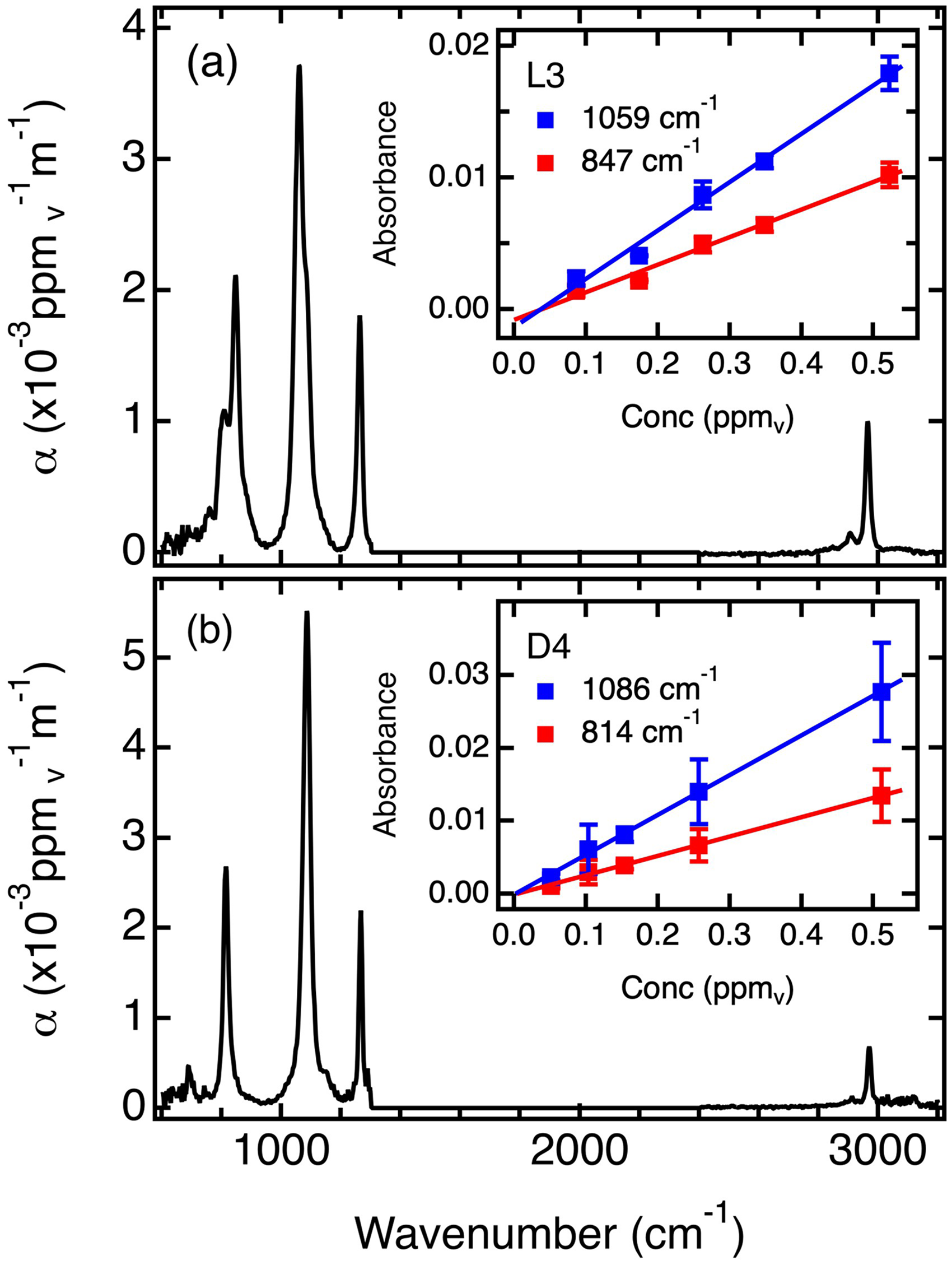
IR absorption spectra of (a) L3 linear siloxane and (b) D4 cyclic siloxane plotted as absorptivity, α, (ppm_v^–1m^–1). The insets show the calibration curves obtained at the peak absorption frequencies of 1059 cm^–1 and 847 cm^–1 for L3 and 1086 cm^–1 and 814 cm^–1 for D4. Water and carbon dioxide absorption bands spanning 1300–2400 cm^–1 have been removed.

Figure 3 also shows representative plots of the calibration data (see insets) obtained at 1059 cm^–1 and 847 cm^–1 for L3 and at 1086 cm^–1 and 814 cm^–1 for D4. Calibrations were performed at every data point between 770 cm^–1 and 1138 cm^–1 at 4 cm^–1 resolution, with the slope of each plot giving the absorptivity data shown. The siloxane concentrations employed ranged from ∼50 ppb_v up to ∼500 ppb_v and were determined as described in supplemental material. The error bars depict the standard deviations obtained from three to four replicate measurements in each case. The entire spectral range (770 cm^–1 to 1138 cm^–1) was employed in the least squares reconstruction of the sample spectrum for siloxane quantification (see below).

Figure 4 shows IR spectra for the model oxygenated VOCs employed. VOC calibrations were performed in a manner identical to siloxane calibration, as described in supplemental material. These spectra were acquired at concentrations of several hundred ppm_v, approximately 10³-fold higher than the concentrations of the siloxanes in the synthetic biogas. Along with their similar methyl stretching bands near 2950 cm^–1 (not shown), all of the VOCs absorb at low frequencies near the siloxane bands. To clearly depict the problems with spectral interference by the VOCs in siloxane determinations, L3 and D4 spectra at 10 ppm_v and 5 ppm_v concentrations, respectively, have been added to each panel in Figure 4. Acetic acid (Figure 4a) has relatively weak absorption bands near 850 cm^–1 and 1060 cm^–1. These directly overlap with the siloxane bands. Acetone (Figure 4b) also exhibits weak absorption bands in this region that interfere with siloxane quantification. The most problematic VOC, however, appears to be ethanol (Figure 4c), which has relatively strong bands near 875 cm^–1 and 1070 cm^–1. Note that at ∼100 ppb_v levels, the siloxane bands will be smaller than the VOC bands and may be entirely obscured by the large ethanol bands in particular. Higher frequency VOC bands (i.e., near 1200 cm^–1) are not considered to be important because the onset of strong methane absorption in this region precludes its use for siloxane quantification. Note that the spectral range shown in Figure 4 is wider than the spectral range used in the analysis, which is to the left of the blue vertical lines appended to the plots.

Figure 4.

IR absorption spectra (solid black lines) for oxygenated VOCs (a) acetic acid (487 ppm_v), (b) acetone (491 ppm_v), and (c) ethanol (315 ppm_v). Overlaid on each plot are the spectra expected for D4 and L3 siloxanes (dashed red lines) at concentrations of 5 ppm_v and 10 ppm_v, calculated from the molecular absorptivity spectra shown in Figure 3. These depict the overlap between the siloxane and VOC absorption peaks. The analysis region employed was to the left of the vertical blue lines (770 cm^–1 to 1138 cm^–1).

Concentrations of Siloxanes and VOCs in the As-Prepared Gas Mixture

For validation of the two-step method, the actual concentrations of the siloxanes in the synthetic biogas mixture were first quantified in pure nitrogen gas alone (without methane or VOCs) using their calibration spectra (Figure 3). Figure 5a shows a representative IR spectrum of the L3 and D4 mixture employed. Superimposed over this spectrum are the least squares reconstructions of pure L3, pure D4, and of the L3/D4 mixture spectra, obtained as described in supplemental material. From these reconstructions, the concentrations of L3 and D4 were determined to be 128 ± 5 ppb_v and 155 ± 5 ppb_v, respectively. These concentrations are provided in Table I for comparison with the concentrations measured later in the synthetic biogas mixture.

Figure 5.

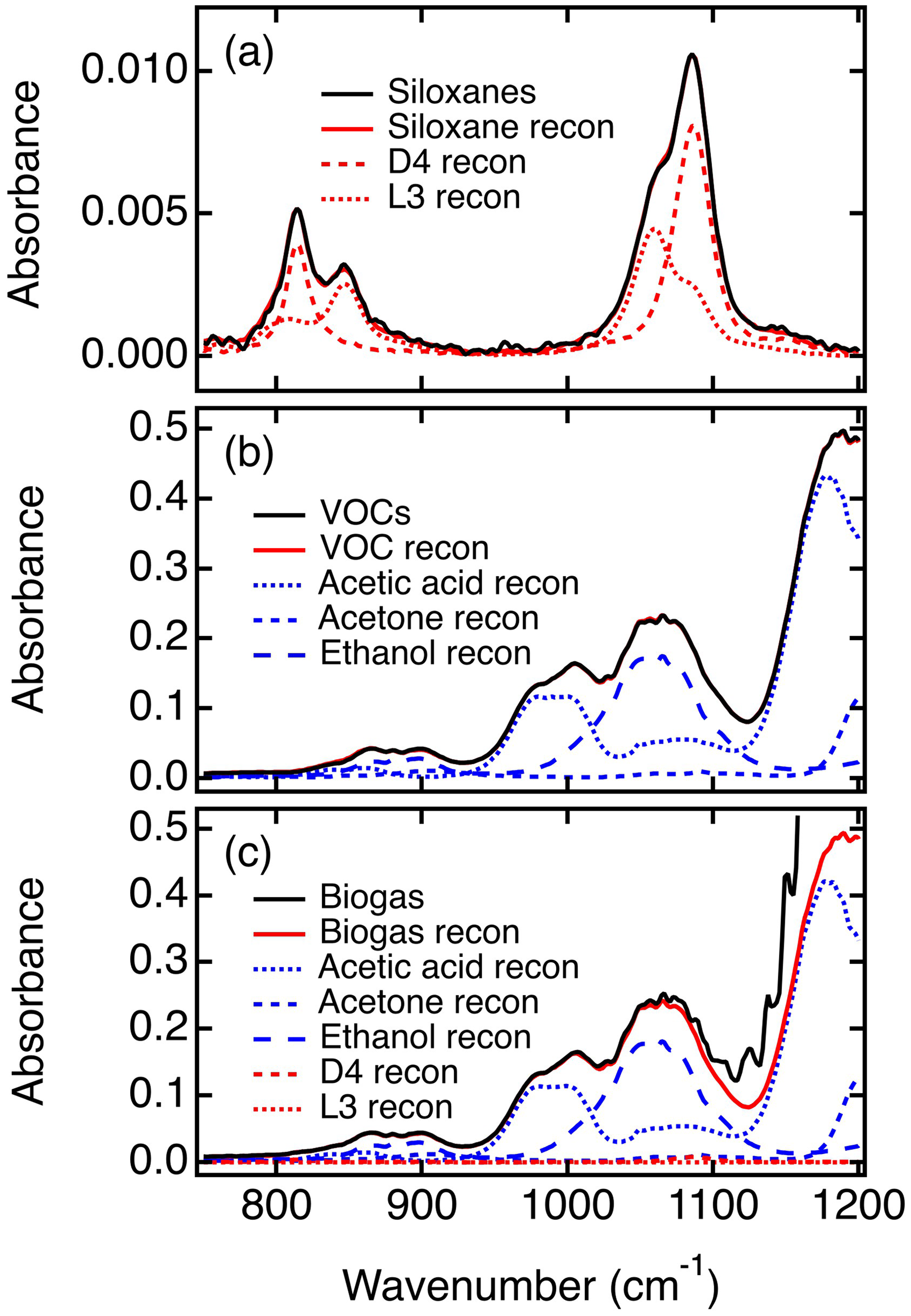
IR spectra of (a) the D4 and L3 siloxane mixture in nitrogen, and (b) the VOC mixture in nitrogen used to establish the concentrations of each component in the synthetic biogas mixture. The concentrations of the siloxanes in (a) were determined by a least squares fitting of the spectrum using the molecular absorptivity data shown in Figure 3. The concentrations of VOCs in (b) were determined by the same method, using molecular absorptivity spectra for these compounds (not shown). (c) Dry synthetic biogas mixture including siloxanes and VOCs at the above concentrations and the least squares fit of the experimental spectrum (Biogas recon). The individual contributions of the VOCs and siloxanes are also shown, demonstrating that the D4 and L3 contributions are masked by the VOC interferents.

Table I.

Siloxane and VOC concentrations and percent recoveries in dry N₂ and N₂/CH₄.

Gas/mixture	L3 (ppb_v)	L3 recov. (%)	D4 (ppb_v)	D4 recov. (%)	Acetic acid (ppm_v)	Acetone (ppm_v)	Ethanol (ppm_v)	Corresponding figure
N₂	128 ± 5	–	155 ± 5	–	–	–	–	Figure 5a
N₂	–	–	–	–	393 ± 18	53 ± 1	137 ± 6	Figure 5b
N₂/CH₄	< 9.3^a	< 7.3^a	154 ± 5	99.4	382 ± 7	56 ± 1	135 ± 6	Figure 5c

These values correspond to the LOD for L3 as given in Table II.

The actual initial concentrations of the VOCs in the biogas mixture were also determined separately in pure nitrogen. Figure 5b shows the spectrum of the VOC mixture along with the reconstructed spectra obtained as described in supplemental material. Using VOC absorptivity data (not shown), the acetic acid, acetone, and ethanol concentrations were determined to be 393 ± 18 ppm_v, 53 ± 1 ppm_v, and 137 ± 6 ppm_v, respectively. Table I also includes these values.

Direct Determination of Siloxanes in the Synthetic Biogas

Following assessment of the siloxane and VOC concentrations in nitrogen, the full gas mixture of siloxanes and VOCs was prepared in 90:10 nitrogen–methane (i.e., dry synthetic biogas). A representative IR spectrum of the dry mixture used in the analysis is shown in Figure 5c. No features associated with the siloxanes are visible in this spectrum because they are masked by the larger methane and VOC absorption bands.

A direct determination of the siloxane content of the dry biogas was first attempted by conducting a simple least squares reconstruction of the spectrum shown in Figure 5c. The equations given in supplemental material (Eq. S3–S5, Supplemental Material) were used in this analysis, along with the siloxane and VOC calibration data, and with a spectrum of the pure nitrogen/methane mixture serving as the blank. This represents the traditional method by which siloxane determination might be performed. The reconstructed spectra of the mixture and its individual components are also shown in Figure 5c. The results yielded an acetic acid concentration of 382 ± 7 ppm_v, an acetone concentration of 56 ± 1 ppm_v, and an ethanol concentration of 135 ± 5 ppm_v. The D4 concentration was found to be 154 ± 5 ppb_v while the L3 concentration was calculated to be < 9.3 ppb_v, its limit of detection (LOD). These results are also included in Table I and are clearly incorrect, due to significant interference by the VOCs. Specifically, much of the L3 concentration is erroneously misassigned to the VOCs due to its overlap with their spectra in general and with the ethanol band near 1070 cm^–1 in particular (see Figure 4c).

Siloxane Concentrations Determined by the Two-Step Method

Significantly improved accuracy in siloxane concentration determinations was achieved when the two-step gas stream modification process was employed. In this process, the biogas was first sparged through water (see Figure 1) to reduce the concentrations of the oxygenated VOCs. Figure 6a shows the spectrum obtained after sparging, representing the wet biogas sample spectrum used in siloxane quantification (see below). Importantly, the siloxane and any remaining VOC spectral features are masked by the much larger contributions of water vapor and methane. A significant reduction in the VOC content occurs upon sparging because of the relatively large Henry's Law constants for these interferents (see Table S1, Supplemental Material). In contrast, the siloxanes pass through the sparging apparatus largely unattenuated due to their much lower solubilities (Table S1).

Figure 6.

(a) IR spectrum (biogas sample) obtained after passage of the gas mixture through the sparging apparatus. The VOCs are mostly removed by sparging while the siloxanes and methane remain. (b) IR spectrum (biogas blank) obtained after passing the sparged gas mixture through the oxidizer module. All remaining VOCs and the siloxanes are removed in the oxidizer module. (c) Siloxane spectrum (solid black line) obtained as the difference between (a) and (b) and simple least squares reconstruction (solid red line) of the siloxane spectrum. (d) Siloxane spectrum (solid black line) obtained as the difference between (a) and (b) with the contributions of residual VOCs removed. Also shown are the siloxane mixture least squares reconstruction (solid red line) and individual D4 and L3 reconstructions (dashed red lines).

After passage of the biogas stream through the sparging apparatus, it was subsequently passed through the low temperature oxidizer module (Figure 1), which removed both the siloxanes and any residual VOCs. The spectrum obtained afterwards, which represents the biogas blank spectrum required for siloxane quantification, is shown in Figure 6b. The spectra shown in Figures 6a and 6b appear to be almost identical, although subtle differences are found in regions where the siloxanes absorb. The difference between these two spectra represents the siloxane spectrum of the biogas mixture. This spectrum is shown in Figure 6c (black line), in which the siloxane bands clearly emerge above the baseline.

The siloxane concentration was determined by performing a least squares reconstruction of the biogas sample spectrum (Figure 6a) using the siloxane calibration spectra (Figure 3) and the biogas blank spectrum (Figure 6b). The reconstructed siloxane spectrum is shown in Figure 6c (red line). This spectrum is similar to the experimental siloxane spectrum in Figure 6c (black line), but the match is imperfect. The siloxane concentrations recovered from this analysis are 149 ± 10 ppb_v and 147 ± 4 ppb_v for L3 and D4, respectively. These are close to the expected values (see Table I) but are still inaccurate. Most significantly, the L3 concentration is higher than the known value (149 ppb_v versus 128 ppb_v). This error arises because the VOCs are not completely removed by sparging and, as noted above, they interfere more significantly with the determination of the L3 concentration than that of D4 (Figure 4c).

To determine the concentrations of VOC interferents remaining after sparging, another least squares reconstruction of the biogas sample spectrum (Figure 6a) was undertaken, this time including the calibration data for the VOCs. The results reveal residual VOC concentrations of 2.4 ± 0.5 ppm_v (0.6% remaining) for acetic acid, 1.7 ± 0.3 ppm_v (3.2% remaining) for acetone, and 0.52 ± 0.04 ppm_v (0.38% remaining) for ethanol. The siloxane concentrations are also obtained in this analysis. The siloxane spectrum and its reconstruction in this case are shown in Figure 6d, after mathematically removing the contributions of the residual VOCs. These spectra are virtually identical to those of the siloxane mixture in nitrogen gas shown in Figure 5a. Quantification of the siloxanes in Figure 6d yielded L3 and D4 concentrations of 119 ± 9 ppb_v and 139 ± 5 ppb_v, respectively. These values are listed in Table II and are only modestly smaller than their concentrations in the original synthetic biogas (Table I), giving 93% recovery for L3 and 90% recovery for D4. These results show that the siloxane concentrations can be accurately determined in mixtures, without interference between the two. The imperfect recovery of the siloxanes could be an artifact of biogas dilution by the incorporation of water vapor during sparging. However, measurements of the water vapor content of the wet biogas reveal it is < 2.5% of the biogas stream by volume. As a result, the errors due to dilution fall within the measurement errors given in Table II and thus cannot be the dominant cause of imperfect siloxane recovery. Furthermore, because of the small errors imparted by dilution of the VOCs and siloxanes in the wet biogas, the results shown in Table II have not been corrected for dilution. Imperfect recovery of the siloxanes is instead attributed primarily to their small solubility in water as reflected by their Henry's Law constants (see Table S1). In this case, the greater recovery of L3 compared to D4 is consistent with its smaller Henry's Law constant, reflecting its lower water solubility.

Table II.

Siloxane and VOC limits of detection, limits of quantification, concentrations and percent recoveries obtained by least squares reconstruction of the spectral data from wet biogas.

Result	L3 (ppb_v)	L3 recov. (%)	D4 (ppb_v)	D4 recov. (%)	Acetic acid (ppm_v)	Acetone (ppm_v)	Ethanol (ppm_v)
LOD	9.3	–	6.3	–	0.392	0.288	0.239
LOQ	31	–	21	–	1.31	0.960	0.797
Recons silox^a	149 ± 10	116	147 ± 4	94.8	–	–	–
Recons all^b	119 ± 9	93.0	139 ± 5	89.7	2.4 ± 0.5	1.7 ± 0.3	0.52 ± 0.04

Results from reconstructed siloxane spectrum in Figure 6c, neglecting the inclusion of residual VOCs.

Results from the reconstructed spectrum in Figure 6d, including VOCs in the calculation.

In real industrial applications of the two-step method reported here, the identity of the VOCs will be unknown, precluding their inclusion in a least squares reconstruction. While the results above show some improvement in L3 quantification with inclusion of the VOCs in the analysis, comparison of the results obtained with and without their inclusion (Table II) suggests that reasonably accurate siloxane quantification can be achieved even when the identities of oxygenated VOC interferents are strictly unknown. In fact, the inaccuracies observed when the VOCs are excluded from the analysis are only two-fold larger than the measurement errors reported in Tables I and II.

Furthermore, industrial applications of the two-step method are likely to use flowing water in place of the static water supply employed for sparging in these studies. The use of flowing water is certain to afford more efficient removal of the VOCs. Deionized water is also unlikely to be employed in the field, where municipal tap water, gray water, or brackish water would be more readily available. In this latter case, additional tests were undertaken to explore VOC removal using municipal tap water and a model for salt water comprised of MgCl₂ dissolved in deionized water. Both the tap water and the MgCl₂ solution were of pH 8.3. The results showed that solutions of ≥0.6 M MgCl₂ resulted in improvements to acetic acid removal but were less effective at removing ethanol and acetone. Municipal tap water performed similarly to deionized water to within experimental error, consistent with the low concentration of ions in the former. Overall, these studies suggest that the use of flowing tap water in place of stagnant deionized water may be the best option for use in industrial applications.

Limits of Detection (LOD) and Quantification (LOQ)

The limits of detection and quantification for siloxanes are critical factors needed for validation of the two-step method. The European Biogas Association specifies a limit of 0.3 mg Si/m³ for biogas that has been upgraded to biomethane.¹³ This corresponds to ∼260 ppb_v volatile Si at 1 atm pressure and 25 °C, requiring maximum concentrations of 87 ppb_v and 65 ppb_v, for L3 and D4, respectively. Estimates of the experimental LOD and LOQ values achieved in these studies were obtained from the errors on the least squares residuals determined by subtracting the experimental siloxane spectrum (black solid line) and the reconstructed siloxane spectrum (red solid line) in Figure 6d. The standard deviation, σ, obtained across the analysis region was determined to be 1.1 × 10^–4 absorbance units. LOD and LOQ values were then calculated as shown in Eqs. 1 and 2, using the siloxane absorptivities, α, at 1059 cm^–1 and 1086 cm^–1 (Figure 3) and the optical path length, b, of 9.86 m.

LOD = \frac{3 σ}{α b}

(1)

LOQ = \frac{10 σ}{α b}

(2)

The LOD and LOQ for L3 were 9.3 ppb_v and 31 ppb_v, respectively, while the LOD and LOQ for D4 were 6.3 ppb_v and 21 ppb_v, respectively. Thus, the two-step gas stream modification method with FT-IR detection readily allows for siloxane detection and quantification at levels well below their specified limits in biogas.

Conclusion

Siloxane contaminants in a synthetic biogas mixture have been successfully detected and quantified in near-real-time by a new gas-phase IR spectrometric method, in the presence of 10³-fold higher concentrations of oxygenated VOCs as spectral interferents. The method was validated using a synthetic biogas mixture comprising linear and cyclic siloxanes (i.e., L3 and D4) with acetic acid, acetone, and ethanol as representative VOCs in a 90:10 mixture of nitrogen and methane. The success of this method relies upon the use of a two-step gas modification process that first removes the VOCs from the gas stream by sparging the biogas through water, allowing for a biogas sample spectrum to be acquired. The gas stream is subsequently passed over a low temperature oxidation catalyst to quantitatively remove the siloxanes and any residual VOCs, allowing for a biogas blank spectrum to be recorded. A least squares analysis is then used to reconstruct the biogas sample spectrum from the biogas blank spectrum and standard spectra of the siloxanes, allowing for quantification of the siloxane concentrations in the biogas. Limits of quantification of 31 ppb_v and 21 ppb_v were obtained for L3 and D4 siloxanes, respectively. These values are far below the levels permitted in biogas by European standards,¹³ demonstrating the efficacy of the method. The demonstration and validation of this method will aid in the development of simple IR instruments for the near-real-time monitoring of siloxanes in industrial biogas streams of unknown composition.

Supplemental Material

sj-pdf-1-app-10.1177_27551857261433051 - Supplemental material for Infrared Quantification of Siloxanes in Synthetic Biogas at Parts-per-Billion Levels in the Presence of Spectral Interferents

Supplemental material, sj-pdf-1-app-10.1177_27551857261433051 for Infrared Quantification of Siloxanes in Synthetic Biogas at Parts-per-Billion Levels in the Presence of Spectral Interferents by Kayla N. McCreary, Nathan J. Ducat, Daniel A. Higgins and Martin L. Spartz in Applied Spectroscopy Practica

Footnotes

Acknowledgments

James Hodgson is thanked for his help in constructing the gas sparging apparatus. Prathap Parameswaran is thanked for helpful discussions during the development of this work.

Data Availability

The data reported here will be made available to interested parties upon request.

Declaration of Conflicting Interests

The authors declared no potential conflicts of interest with respect to the research, authorship, and/or publication of this article.

Funding

Ellington Valley Consulting, LLC (EVC) is thanked for providing financial support for this work. Martin L. Spartz of EVC contributed to the experimental design, performance of the experiments, and analysis and interpretation of the data obtained.

ORCID iDs

Daniel A. Higgins

Martin L. Spartz

Supplemental Material

All supplemental material mentioned in the text accompanies the published version of this work.

References

Rasi

Läntelä

Rintala

. “Trace Compounds Affecting Biogas Energy Utilisation: A Review”. Energ. Convers. Manage. 2011. 52(12): 3369–3375. 10.1016/j.enconman.2011.07.005.

Rafiee

Khalilpour

K.R.

Prest

Skyrabin

. “Biogas as an Energy Vector”. Biomass Bioenerg. 2021. 144: 105935. 10.1016/j.biombioe.2020.105935.

Rivera-Montenegro

Valenzuela

E.I.

González-Sánchez

Muñoz

, et al. “Volatile Methyl Siloxanes as Key Biogas Pollutants: Occurrence, Impacts and Treatment Technologies”. Bioenerg. Res. 2023. 16(2): 801–816. 10.1007/s12155-022-10525-y.

Pascual

Lebrero

Cantera

. “Toward a Sustainable and Cost-Efficient Biological-Based Platform for Siloxanes Removal”. Crit. Rev. Environ. Sci. Technol. 2023. 53(1): 70–86. 10.1080/10643389.2022.2044254.

Schweigkofler

Niessner

. “Removal of Siloxanes in Biogases”. J. Hazard. Mater. 2001. 83(3): 183–196. 10.1016/S0304-3894(00)00318-6.

Dewil

Appels

Baeyens

. “Energy Use of Biogas Hampered by the Presence of Siloxanes”. Energ. Convers. Manage. 2006. 47(13-14): 1711–1722. 10.1016/j.enconman.2005.10.016.

de Arespacochaga

Valderrama

Raich-Montiu

Crest

, et al. “Understanding the Effects of the Origin, Occurrence, Monitoring, Control, Fate, and Removal of Siloxanes on the Energetic Valorization of Sewage Biogas: A Review”. Renew. Sust. Energ. Rev. 2015. 52: 366–381. 10.1016/j.rser.2015.07.106.

Mendiara

Cabello

Izquierdo

M.T.

Abad

, et al. “Effect of the Presence of Siloxanes in Biogas Chemical Looping Combustion”. Energy Fuels. 2021. 35(18): 14984–14994. 10.1021/acs.energyfuels.1c02031.

Alves

C.M.A.C.

Abreu

F.O.M.S.

Araujo

R.S.

Oliveira

M.L.M.

. “Recent Advances in Siloxanes Removal from Biogas and Their Efficiency: A Short Review”. Chem. Pap. 2023. 77: 1–9. 10.1007/s11696-022-02460-1.

10.

Vali

S.A.

Moral-Vico

Font

Sánchez

. “Adsorptive Removal of Siloxanes from Biogas: Recent Advances in Catalyst Reusability and Water Content Effect”. Biomass Convers. Biorefin. 2024. 14: 23259–23273. 10.1007/s13399-023-04478-1.

11.

Golmakani

Nabavi

S.A.

Wadi

Manovic

. “Advances, Challenges, and Perspectives of Biogas Cleaning, Upgrading, and Utilisation”. Fuel. 2022. 317: 123085. 10.1016/j.fuel.2021.123085.

12.

Raich-Montiu

Ribas-Font

de Arespacochaga

Roig-Torres

, et al. “Analytical Methodology for Sampling and Analysing Eight Siloxanes and Trimethylsilanol in Biogas from Different Wastewater Treatment Plants in Europe”. Anal. Chim. Acta. 2014. 812: 83–91. 10.1016/j.aca.2013.12.027.

13.

Royal Netherlands Standardization Institute (NEN). “Natural Gas and Biomethane for Use in Transport and Biomethane for Injection in the Natural Gas Grid”. NEN-EN 16723-1 and EN 16723-2”. https://www.nen.nl/en/nen-en-16723-1-2016-en-227030 [accessed 27 February 2026].

14.

Santos-Clotas

Cabrera-Codony

Boada

Gich

, et al. “Efficient Removal of Siloxanes and Volatile Organic Compounds from Sewage Biogas by an Anoxic Biotrickling Filter Supplemented with Activated Carbon”. Bioresour. Technol. 2019. 294: 122136. 10.1016/j.biortech.2019.122136.

15.

Shen

Zhang

Fan

, et al. “A Review on Removal of Siloxanes from Biogas: With a Special Focus on Volatile Methylsiloxanes”. Environ. Sci. Pollut. Res. 2018. 25(31): 30847–30862. 10.1007/s11356-018-3000-4.

16.

Arnold

Kajolinna

. “Development of On-Line Measurement Techniques for Siloxanes and Other Trace Compounds in Biogas”. Waste Manage. 2010. 30(6): 1011–1017. 10.1016/j.wasman.2009.11.030.

17.

Hepburn

C.A.

Vale

Brown

A.S.

Simms

N.J.

, et al. “Development of On-Line FTIR Spectroscopy for Siloxane Detection in Biogas to Enhance Carbon Contactor Management”. Talanta. 2015. 141: 128–136. 10.1016/j.talanta.2015.03.063.

18.

Aydın Kızılkaya

Y.M.

Uyak

. “Adsorptive Puriﬁcation of Volatile Methyl Siloxanes in a Digester Biogas Stream”. J. Chem. Technol. Biotechnol. 2021. 96(11): 3084–3093. 10.1002/jctb.6860.

19.

Braganca

Sanchez-Soberon

Pantuzza

G.F.

Alves

, et al. “Impurities in Biogas: Analytical Strategies, Occurrence, Effects and Removal Technologies”. Biomass Bioenergy. 2020. 143: 105878. 10.1016/j.biombioe.2020.105878.

20.

Lecharlier

Carrier

Hecho

I.L.

. “Characterization of Biogas and Biomethane Trace Compounds: A Critical Review of Advances in Situ Sampling and Preconcentration Techniques”. Anal. Chim. Acta. 2022. 1229: 340174. 10.1016/j.aca.2022.340174.

21.

Ghidotti

Fabbri

Torri

. “Determination of Linear and Cyclic Volatile Methyl Siloxanes in Biogas and Biomethane by Solid-Phase Microextraction and Gas Chromatography-Mass Spectrometry”. Talanta. 2019. 195: 258–264. 10.1016/j.talanta.2018.11.032.

22.

Piechota

. “Siloxanes in Biogas: Approaches of Sampling Procedure and GC-MS Method Determination”. Molecules. 2021. 26(7): 1953. 10.3390/molecules26071953.

23.

Foppiano

Tarik

Schneebeli

Calbry-Muzyka

, et al. “Siloxane Compounds in Biogas from Manure and Mixed Organic Waste: Method Development and Speciation Analysis with GC-ICP-MS”. Talanta. 2020. 208: 120398. 10.1016/j.talanta.2019.120398.

24.

Wang

Liao

Wang

. “Influence of Sampling Methods and Storage Condition on Volatile Methyl Siloxanes Quantification in Biogas”. Biomass Bioenergy. 2022. 158: 106347. 10.1016/j.biombioe.2022.106347.

25.

Oshita

Ishihara

Takaoka

Takeda

, et al. “Behaviour and Adsorptive Removal of Siloxanes in Sewage Sludge Biogas”. Water Sci. Technol. 2010. 61(8): 2003–2012. 10.2166/wst.2010.101.

26.

Adekunle

K.F.

Okolie

J.A.

. “A Review of Biochemical Process of Anaerobic Digestion”. Adv. Biosci. Biotechnol. 2015. 6(3): 205–212. 10.4236/abb.2015.63020.

27.

Goswami

Chattopadhyay

Shome

Banerjee

S.N.

, et al. “An Overview of Physico-Chemical Mechanisms of Biogas Production by Microbial Communities: A Step Towards Sustainable Waste Management”. 3 Biotech. 2016. 6(1): 72. 10.1007/s13205-016-0395-9

28.

Bernard

Papanastasiou

D.K.

Papadimitriou

V.C.

Burkholder

J.B.

. “Infrared Absorption Spectra of Linear (L₂–L₅) and Cyclic (D₃–D₆) Permethylsiloxanes”. J. Quant. Spectrosc. Radiat. Transfer. 2017. 202: 247–254. 10.1016/j.jqsrt.2017.08.006.

Supplementary Material

Please find the following supplemental material available below.

For Open Access articles published under a Creative Commons License, all supplemental material carries the same license as the article it is associated with.

For non-Open Access articles published, all supplemental material carries a non-exclusive license, and permission requests for re-use of supplemental material or any part of supplemental material shall be sent directly to the copyright owner as specified in the copyright notice associated with the article.

0.00 MB

0.58 MB