
Abstract
Wavelength calibration of linear array spectrometers is conventionally performed by fitting a polynomial function of pixels to calibration data consisting of spectral lines with known wavelengths and their pixel locations. Alternatively, a multiparameter physical model of the optical system can be constructed and the parameters optimized to reproduce the calibration data. Here, a new spectrometer wavelength calibration method is introduced with two distinguishing features: the reference calibration points are treated as fixed points, and are used as nodes for cubic Hermite spline interpolation between those points. Conveniently, in the Hermite form of cubic splines, the calibration data, i.e., the calibration wavelengths together with the slopes at those calibration points, explicitly appear as the parameters of the interpolating functions. The slopes are derived from the grating equation and the physical model of the optical system. As a result, the calibration curve is fully determined without the need for intermediate calculations such as polynomial regression or model parameter fitting. Zero residual error is ensured at those reference points and interpolation errors in the intervals between reference points are very low, approaching the limit of spectral line peak location uncertainty. The calibration procedure is demonstrated for a compact flat-field spectrometer. This method improves and simplifies the spectrometer wavelength calibration procedure and offers a convenient method of calibration for systems with limited computing resources.
This is a visual representation of the abstract.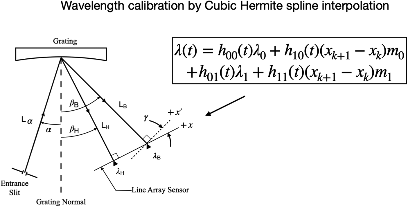
Keywords
Introduction
Spectrometers with linear array sensors, such as photodiode or charge-coupled device (CCD) pixel sensors, simultaneously measure the diffracted light intensity for a range of wavelengths. Sensor array spectrometers have an advantage over scanning monochromators with their high-speed acquisition of spectra making them suitable for applications with fast evolving or transient spectra such as fluorescence and luminescence, real-time monitoring of process spectra, plasma diagnostics, and others.
In sensor array spectrometers, wavelength calibration is the process of assigning the correct wavelength to the pixel location to ensure the accuracy of the spectrometer. To calibrate a spectrometer, a gas-discharge calibration lamp is used as a light source. From the measured spectrum, the pixel locations of the known atomic emission spectral lines of the lamp are determined. Conventionally, a polynomial function is fit to the wavelength-pixel calibration data. Alternatively, an optical model of the spectrometer is constructed with parameters relating to the optical components to predict the wavelengths as a function of pixel location. Then a model parameter fitting procedure, such as a least-squares method, is performed to match the calibration data. These calibration methods and the history of wavelength calibration are thoroughly discussed by Liu and Hennelly 1 and the references cited therein.
In this work, a new method of wavelength calibration is introduced, based on cubic Hermite spline interpolation, and demonstrated on a compact flat-field spectrometer. The method treats the calibration points as fixed points and uses spline interpolation between those points. The interpolating functions are cubic polynomials expressed in terms of Hermite basis functions. This method simplifies the calibration procedure, eliminates residual errors at the reference wavelength pixel locations, and improves interpolation errors.
An important feature of this calibration procedure is that the interpolating functions are completely determined by the calibration points themselves and the slopes (wavelength linear dispersion) which are derived from the grating equation and spectrometer geometry. The calculation method is explicit, work-flow efficient and unlike polynomial regression or model parameter fitting, there is no need for an intermediate computation to arrive at the calibration function.
Additionally (although most control and computing systems for spectrometers have enough computing power to carry out calculations for calibration procedures), there may be special cases where this calibration method can be useful for spectrometer systems with very limited computing resources. Examples are embedded systems or where system autonomy is required, such as on-board systems used in space probes or robotic roving vehicles for planetary exploration or operation in harsh environments.
Background
Calibration Procedure
To calibrate spectrometers with photosensor arrays, a lamp with known spectral lines is used (for example, a mercury-argon calibration lamp with spectral lines in the visible spectral region). The wavelengths of these spectral lines are known accurately 2 with a precision of 10−4 nm. The light output of the calibration lamp is collected by the spectrometer. The spectral lines are identified and their pixel locations determined. Then a calibration curve is generated from these calibration data points.
Polynomial Fitting and Optical System Modeling
One method of determining the wavelength calibration curve is to express the wavelength as a polynomial function of pixels. A set of
A different method of wavelength calibration is to simulate the behavior of the spectrometer using a model of the optical system. This is in contrast to the polynomial method, which is a straightforward approach in which the wavelength is expressed as an expansion of the pixel variable. Not all of the parameters in the polynomial method correspond to the physical or optical parameters in the spectrometer system except in the simplest case of a linear model. The complexity of the optical model corresponds to the complexity of the optical design of the spectrometer.
In the simplest optical model, the wavelengths are determined directly from the grating equation 3 and by calculating the linear dispersion across the array (these will be discussed in another section as they are also used as the basis for the method introduced in this work). This approach was used in Gaigalas et al. 4 for a hybrid spectrometer system consisting of a scanning monochromator with a CCD sensor array positioned in place of the exit slit. They used an array sensor 27 mm long, which is much less than the spectrometer focal length of 270 mm. To speed up data acquisition, the full spectrum (420–840 nm) is obtained by splicing partial spectra of 60–80 nm widths acquired by the array while rotating the grating at 5–6 predetermined discrete angles to cover the entire spectrum.
For more complex spectrometer optics and a wider wavelength coverage, a full optical modeling approach is used, where the wavelength-dispersing optical element (grating) and the input and output optics are modeled together to simulate the wavelength dispersion along the linear axis occupied by sensor array pixels.
The optical system parameters are then optimized so that the modeled dispersion matches the calibration data, as was done by Liu and Hennelly 1 and others cited in their study. In that example, the full optical model used six parameters related to the grating, and the spectrometer and camera geometry. However, for faster calculations, only three optical parameters were varied in a least-squares fitting procedure to determine those three parameters. The rest of the parameters were fixed. Mathematically, this is equivalent to a polynomial fit to the calibration data, except that the model parameters correspond to the physical parameters of the spectroscopic system.
An even more complicated model-based approach is described by Dorner et al. 5 for the NIRSpec spectrometer onboard the James Webb Space Telescope. A full parametric optomechanical model of the NIRSpec optical system was constructed (similar to a digital twin), taking into account all of the optical elements to simulate the location of the spectral lines on the detector. An iterative process was then carried out consisting of a manual parameter adjustment and an optimization procedure to match the wavelength calibration data.
Calibration Data as Fixed Points
The reported error in the wavelength values of the calibration spectral lines 2 is on the order of 10−4 nm, nearly zero relative to the residual error of a polynomial fit and the position error of the peak of the spectral line. The calibration spectral lines can therefore be treated as fixed points with zero error in the sense that the calibration curve should pass through those calibration points.
The use of fixed points in wavelength calibration is analogous to the use of thermodynamic fixed points in establishing the International Temperature Scale of 1990 (ITS-90), adopted by the International Committee on Weights and Measures in 1989.
6
ITS-90 is defined for a wide temperature range from 0.65 K to more than 961.78 °C. It has several sub-ranges and uses several fixed points spanning the temperature range. These thermodynamic fixed points consist of vapor pressure points, triple points, and melting and freezing points of several substances. To determine the temperature for each subrange between fixed points, an interpolating function is used that is based on a temperature-dependent property of the physical system of the thermometry method, such as pressure for a
It is worth noting that in the new calibration method to be discussed here, the interpolating function is also based on a physical model of the optical system. This is another aspect of the calibration method that is analogous to the approach developed for ITS-90 thermometry.
Cubic Spline Interpolation
One method of finding a polynomial function that passes through the calibration points is the Lagrange method. However, the polynomial found using that method is prone to oscillations between points resulting in large interpolation errors. A better method to use which avoids these oscillations is the cubic spline interpolation, 7 a piecewise polynomial interpolation method where the calibration points are the nodes with a cubic polynomial interpolation function between them. The cubic polynomials are subject to the conditions that the functions are continuous and the first and second derivatives are continuous at the nodes. These conditions, together with additional constraints imposed by the choice of boundary conditions, result in a set of equations represented in matrix form. This matrix equation is then solved to determine the cubic spline polynomial coefficients.
Cubic Hermite Splines
One form of the cubic spline interpolation method is the cubic Hermite spline (CHS) interpolation, where the interpolating functions are written in terms of a linear combination of Hermite basis functions.7,8 Interestingly, the coefficients of the Hermite functions turn out to be the calibration points and the slopes at the nodes. These parameters appear explicitly in the interpolating functions without the need for additional computations such as the polynomial regression, model parameter-fitting or matrix inversion (for the polynomial fitting, physical/optical model, and standard cubic spline interpolation methods, respectively) to construct the calibration curve.
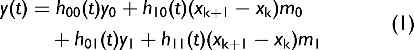
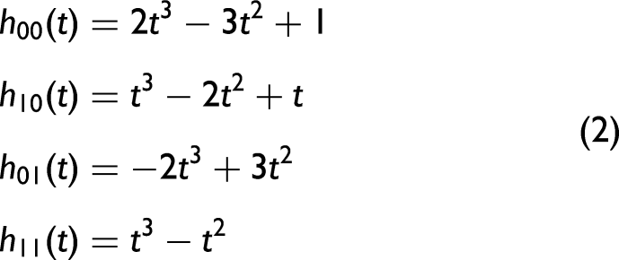
In the CHS formulation, the form of the interpolating polynomial
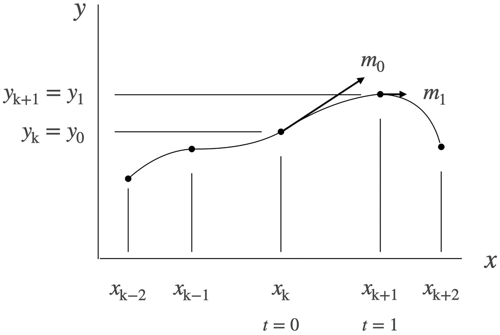
Cubic Hermite Spline method showing nodes
Writing Eq. 1 in terms of the wavelength-pixel values (
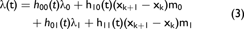
It can be seen from Eq. 3 that the set of three-valued calibration points
Determination of the Slopes
The slopes can be determined from the optical model of the spectrometer system. The slope is the wavelength dispersion along the pixel direction of the array sensor and is derived from the grating equation. Other approximate methods to calculate the slopes will be discussed, including finite difference methods such as the forward-backward finite difference and the related method of Catmull-Rom cubic splines.
To derive the linear wavelength dispersion along the axis of the pixels, consider a diffraction grating with incident and diffracted light rays shown in Figure 2. For this arrangement, the grating equation is

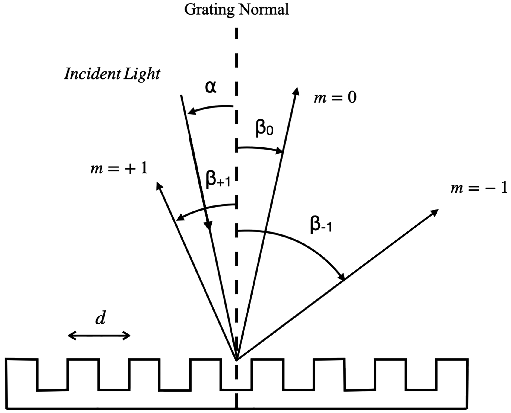
Plane diffraction arrangement.
For an incident angle
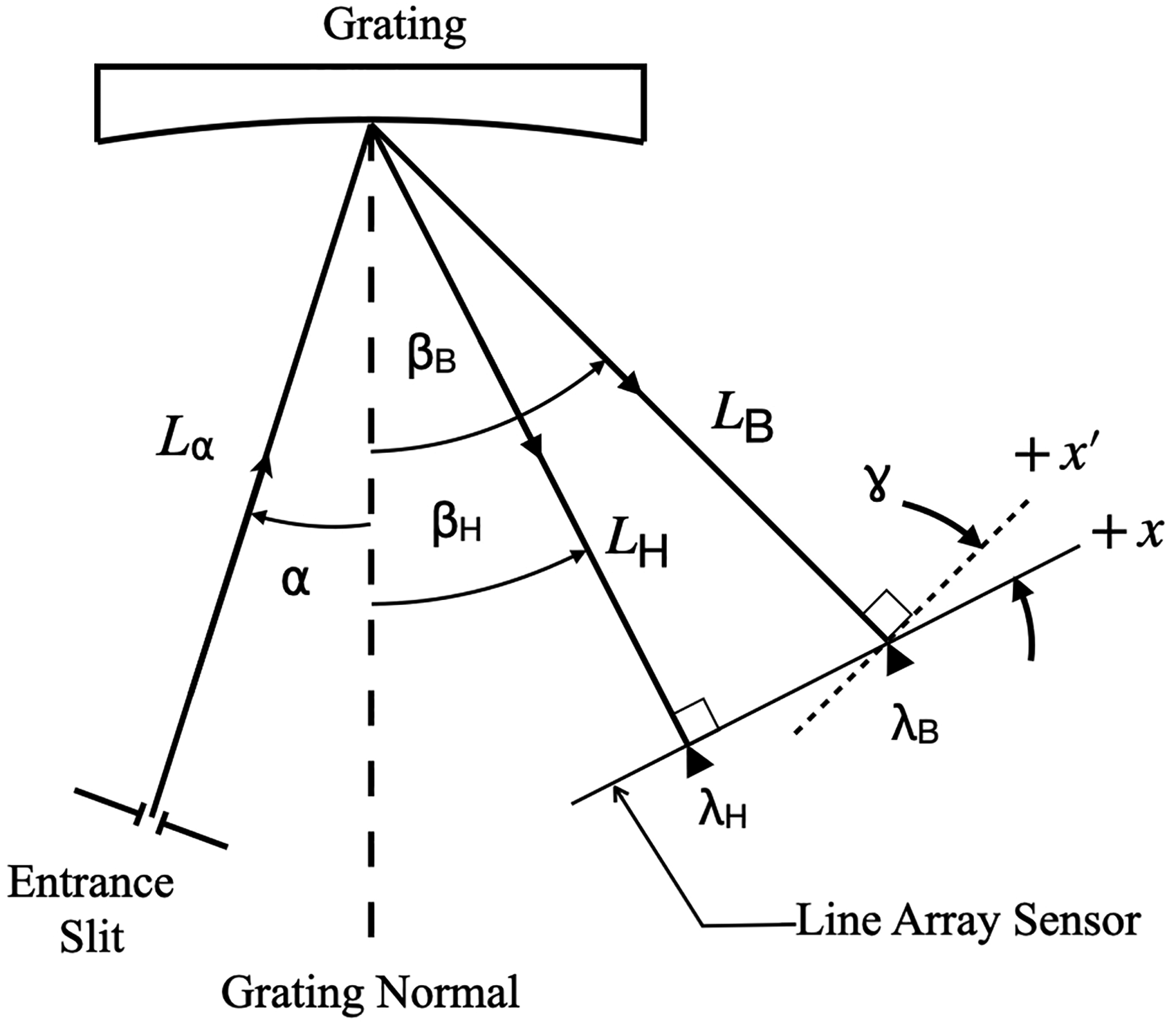
Optical arrangement for a flat-field concave grating spectrometer.
The coordinate
In Figure 3, the focal points of the diffracted rays define a line that coincides with the array sensor designated as
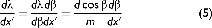
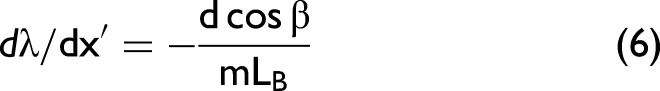
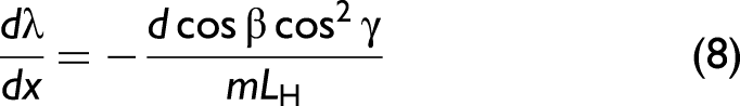
The local dispersion at an angle
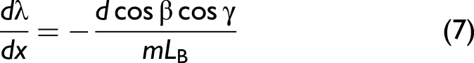
In Eq. 7 ,
Materials and Methods
Spectrometer
The CHS wavelength calibration method was studied using calibration data from a compact spectrometer that uses an imaging type flat-field concave grating (aberration-corrected toroidal grating, Shimadzu Corporation, model no. P0550-02TR) as the single optical element that disperses the incoming light into its various wavelength components and focuses the diffracted light onto the array. The toroidal surface profile of the grating corrects for the aberration. The grating line spacing is also variable to further improve the aberration performance. The simplicity of the optical system allows for a test of the proposed calibration method.
The grating has a groove density of 550 grooves/mm at the center of the grating, an average dispersion of 18.1 nm/mm, and dimensions of 30 × 30 mm. The rest of the specifications of this concave grating are summarized in Table 1. The focal plane is normal to the focal length and angle pair
Summary of toroidal grating Specifications a .
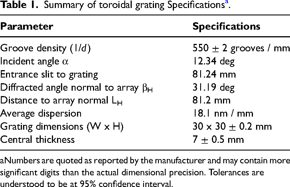
Numbers are quoted as reported by the manufacturer and may contain more significant digits than the actual dimensional precision. Tolerances are understood to be at 95% confidence interval.
The compact spectrometer uses a photodiode array sensor (Hamamatsu Photonics model no. S11639-01 CMOS linear image sensor) with 2048 pixels. Each pixel is 14
The width of the entrance slit was 50
Calibration Spectral Lines and Pixel Location
Calibration spectral data was obtained from a mercury–argon (Hg–Ar) spectral calibration lamp. This lamp has many spectral lines in the ultraviolet (UV), visible (Vis), and near-infrared (NIR) wavelength regions suitable for use in wavelength calibration. A total of 10 isolated peaks were selected for use in calibration. The pixel positions of the spectral lines were located to subpixel precision using the centroid method4,9 shown in Eq. 9. The peak pixel location is calculated as a weighted average of the pixels (with light intensity as the weighting distribution) within a window 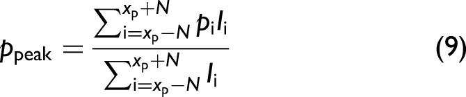
The numerical error in locating the pixel location of the peak using the centroid method is dependent on the signal-to-noise ratio (SNR). For a spectrometer with an SNR of 250 at full count and a window of the size of one FWHM, 9 this error is estimated to be of the order of 0.01 pixel (about 0.0025 nm when multiplied by the wavelength linear dispersion). For typical peaks that are lower than the full signal count of the photodiode array, for which the estimated SNR is 50, a typical pixel location error would be 0.05 pixel, equivalent to about 0.0125 nm. This numerical error is not the main contributor to the pixel location error as it is much less than the physical optical resolution of the optical system of the spectrometer, estimated to be 0.14 pixel (0.036 nm) at the center of the spectrum and 0.23 pixel (0.052 nm) at the long wavelength end of the spectrum. In the centroid method, the numerical error is negligible as a source of error for the peak location.
The centroid method works well for isolated spectral lines. For doublets where there is more separation between the doublet lines, only one line is used for calibration, and the centroid method is applied to that line by limiting the centroid calculation to a range of pixels around its peak equivalent to one FWHM.
The pixel positions of these spectral lines found using the centroid method are then assigned to the reference values of the appropriate Hg or Ar emission lines. 2 From this wavelength-pixel data-set, a calibration curve is constructed that converts pixels to wavelength values.
Polynomial Fitting
The wavelength is modeled by a polynomial function of pixel of the form
The deviations are a measure of the error random variable
Cubic Hermite Spline Interpolation
As shown in Eq. 3, the coefficients of the Hermite functions in the CHS interpolation are determined from the pixel locations of the calibration spectral lines (the nodes), the values of the calibration wavelengths, and the slopes at those calibration wavelengths. The slopes are calculated from Eq. 8 using the dimensions of the spectrometer in Table 1. The calibration curve is thus explicitly constructed, and no further calculation step is needed to determine the calibration curve.
The
To estimate the mean interpolation error, a “Leave one out” cross-validation (LOOCV) procedure was adopted similar to that discussed in Liu and Hennelly
1
and Henriksen et al.
14
In this procedure, an interior calibration point is removed from the calibration data set, and the CHS interpolating function is constructed using the two calibration points (nodes) adjacent to the one removed. The wavelength at the pixel location of the calibration point that was removed is interpolated and its deviation from the calibration value is calculated. This process is then repeated for every interior calibration point. An error metric, which we denote as interpolated residual standard error (
This
In addition, an actual CHS calibration will use all the calibration points, and therefore the true interpolation error will be smaller than this
Results and Discussion
Results of the Polynomial Method
The third-order polynomial fit to the calibration data and its residuals are shown in Figure 4. The fitting and associated statistics were performed using R software.
15
The third-order polynomial fit result was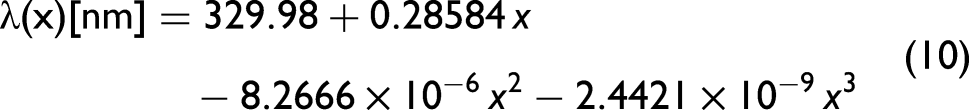
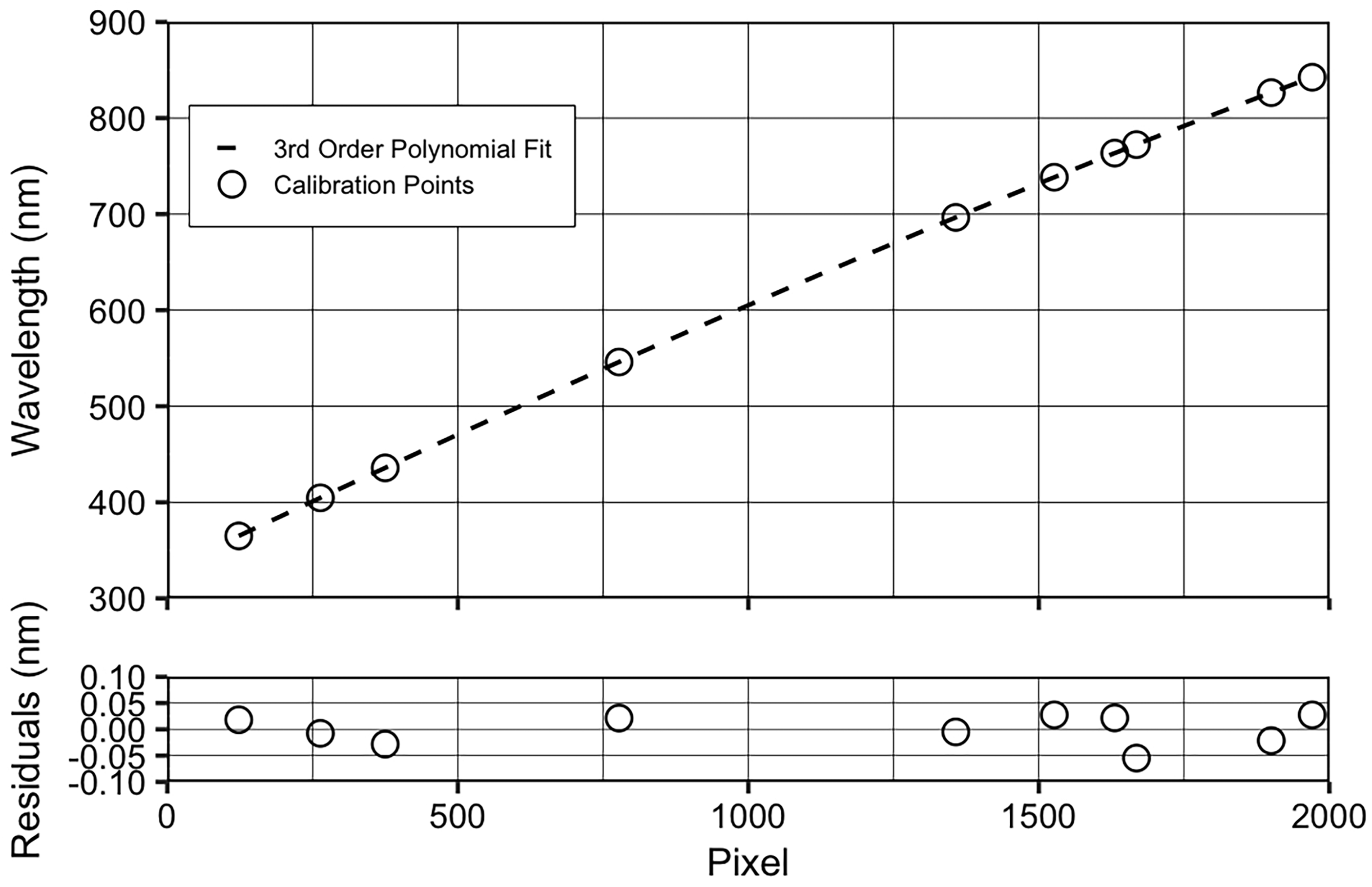
The third-order polynomial fit (top) and the residuals (bottom).
The R analysis is only briefly discussed here. The reported residual standard error (
Most wavelength calibration procedures for spectrometers using polynomial fitting report only the
Furthermore,
Cubic Hermite Spline Method Using Slopes Derived from Grating Equation
The CHS model (referred to simply as CHS) interpolation method takes as the parameters the pixel locations, the wavelengths of the calibration spectral lines, and the wavelength linear dispersion (slopes) at those wavelengths. Those parameters explicitly appear in the Hermite form of the interpolation function shown in Eq. 3. The slopes at the nodes
The CHS slopes calculated from the optical model and finite difference approximations.
To estimate the mean interpolation error, the leave-one-out cross-validation (LOOCV) procedure described previously was used. The method removes a calibration point from the calibration data set, which is then interpolated using the remaining calibration points. The deviation between the known wavelength and the interpolated wavelength was then calculated for each interior point. Using this procedure and calculating the error for all interior points, the
This
The results of the CHS method with slopes calculated from the optical model are summarized in Table II together with the results of the polynomial fit for comparison.
Summary of error metrics (in nm).

Cubic Hermite Spline Method Using Slopes Approximated by Finite Differences (Forward and Backward)
The slopes 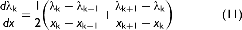
For the first and last nodes, the slopes can be approximated by the forward and backward finite differences respectively. Using these approximated slopes as parameters for the CHS, the
Cubic Hermite Spline Method Using Slopes Approximated by Central Finite Differences (Catmull-Rom splines)
Another way to approximate the slope at a node is to calculate the slope of the line that connects the previous node to the next node. This is a central difference method similar to the Catmull–Rom spline (CRS)
16
(although strictly speaking, this method is for equally spaced intervals). Using this generalized CRS approach, the slope at node 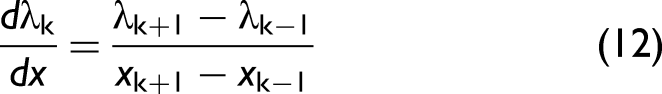
The
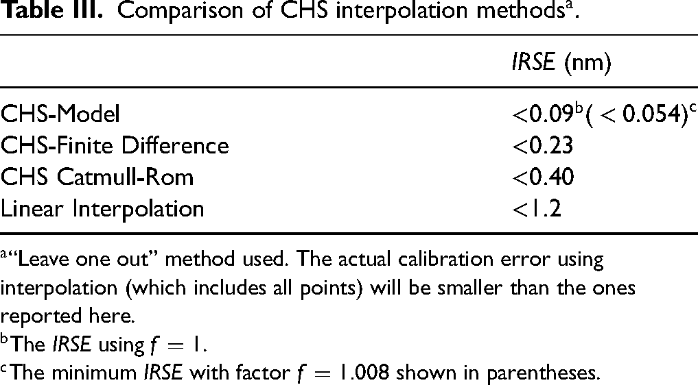
The results of the CHS using these slope determination methods are summarized in Table III, which includes results using linear interpolation for the slope approximation.
Comparison of CHS interpolation methods
Analysis
Contribution of Slope Calculation Errors to Interpolation Errors
The CHS 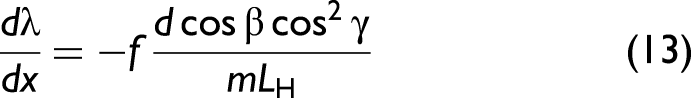
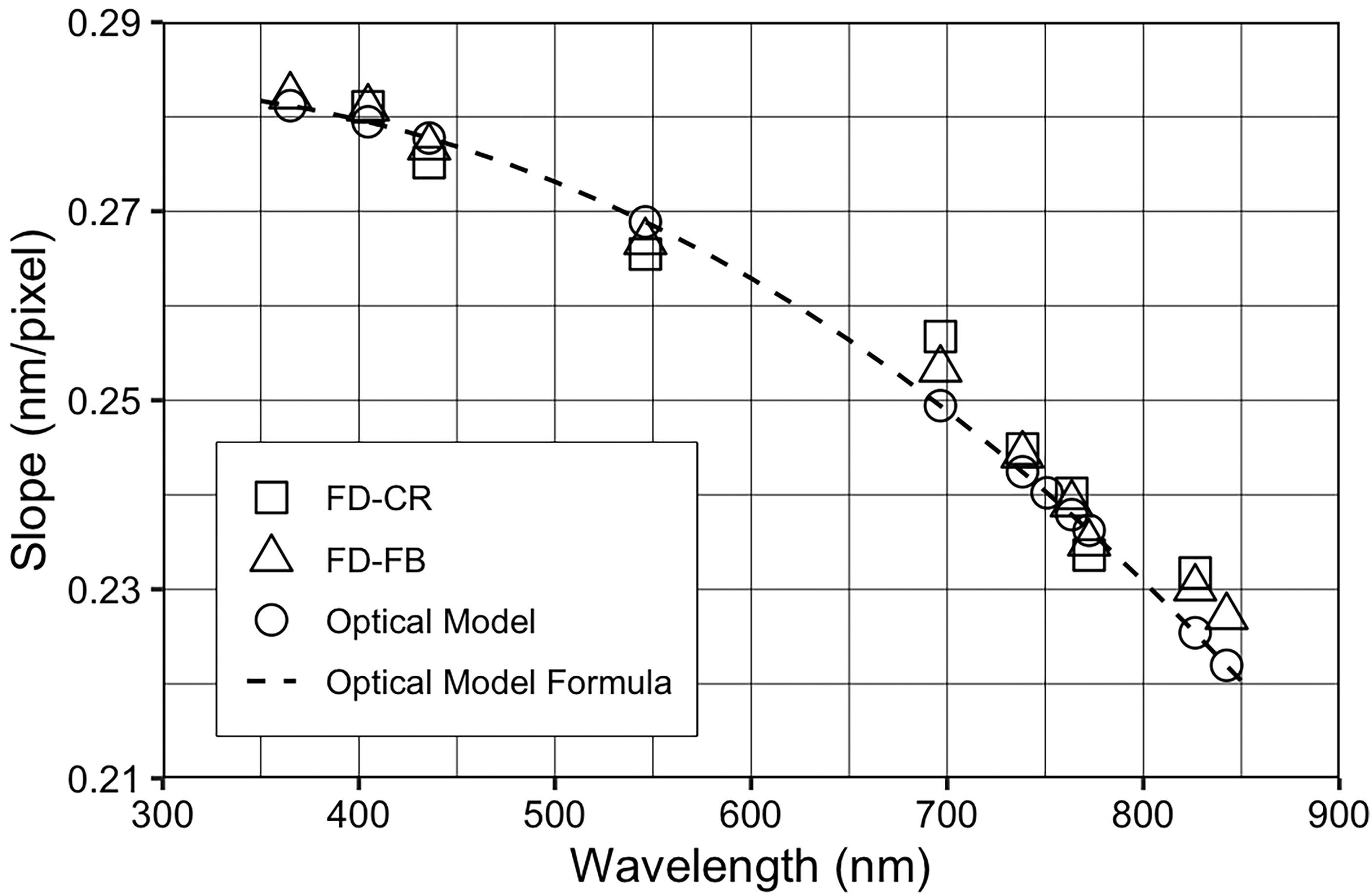
The slopes were determined in several ways: the slope calculated from the optical model and spectrometer geometry, the slope approximated using forward and backward finite difference, and the CRS or central finite difference. The slopes calculated using these different methods are shown in Figure 5. The finite difference and CRS approximations differ from the optical model (CHS) with the CR approximation being worse than the forward-backward finite difference.
The deviations between the predicted (interpolated) wavelengths and the known wavelengths were calculated using these different slope calculation methods. Figure 6 shows a plot of the deviations versus the interpolation interval between nodes. The deviation from a calibration using linear interpolation is also included for comparison. The CHS method has the smallest interpolation deviations. As expected, when the slopes are approximated, the interpolation deviations increase as the interval between the nodes increases. At larger intervals, the deviation is smaller for the forward-backward method compared with the CRS or central difference method, indicating a better approximation of the slopes. This underscores the importance of accurately determining the slope. Interestingly, for CHS using slopes derived from the optical model, the deviation does not increase as the interpolation interval increases (at least with the calibration data studied here). This suggests that the interpolation remains accurate even with wider node spacing.
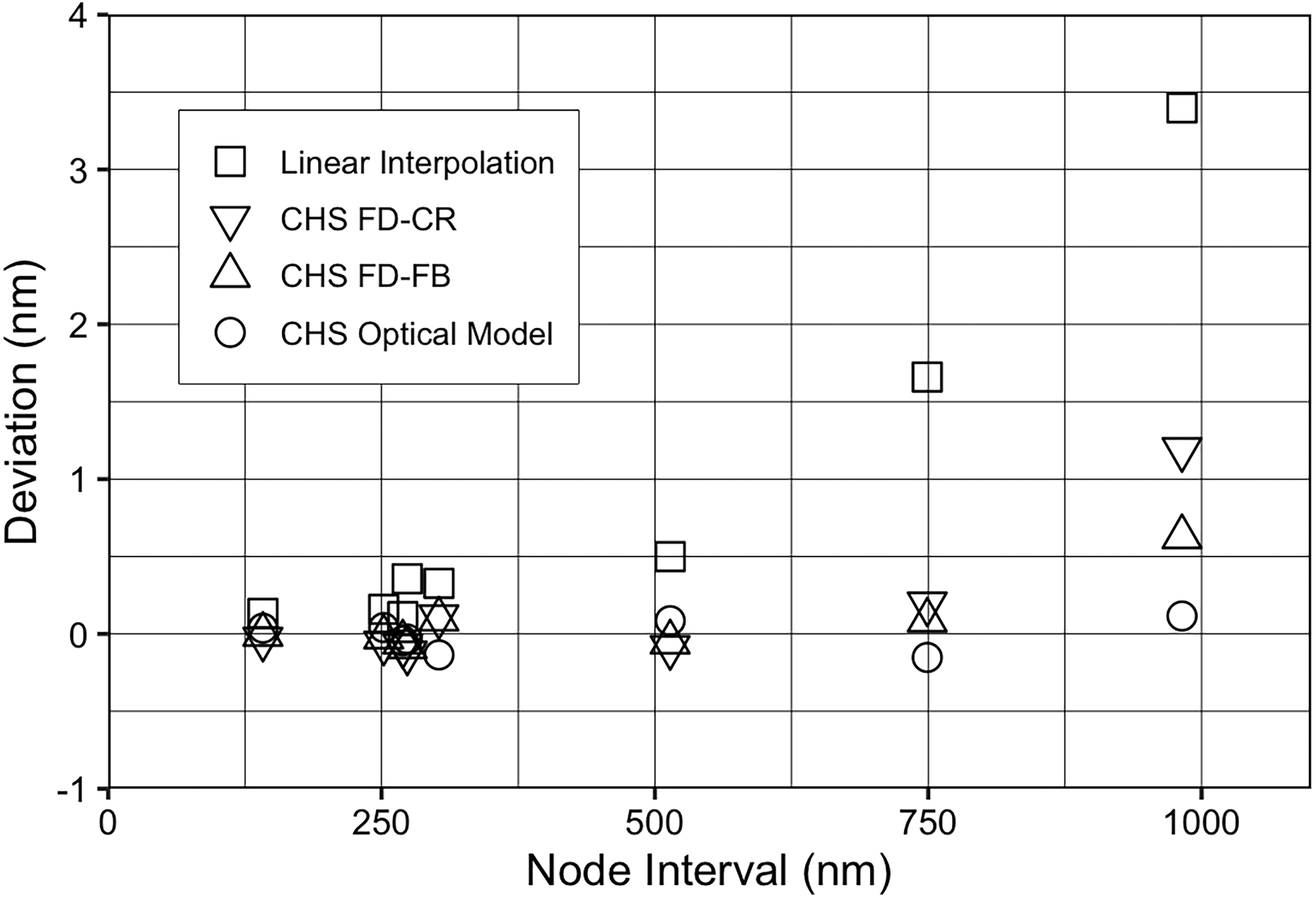
Deviation of predicted/interpolated wavelength from the calibration value versus node interval, using the LOOCV procedure; CHS interpolation with slopes calculated using several methods are shown.
In discussions of conventional polynomial fitting calibration procedures, wavelength uncertainties in the calibration points are not considered, and expanded errors in the predicted wavelengths from the calibration curves are often also overlooked. In this study, we have discussed the latter by calculating the prediction intervals for the polynomial fitting error. To make a direct comparison with the polynomial method, the former uncertainty is not considered in the CHS as well.
The wavelength uncertainties are relatively easier to take into account if they are random and can be treated statistically. However, sources of uncertainties such as those coming from aberrations are more computationally demanding to address as they are wavelength dependent. Presumably, a deconvolution procedure might be useful, as was done, for example, by Koike and Oshio. 17
Computational Complexity of Calibration and Recalibration
The polynomial fitting method used to determine the calibration curve is more mathematically complex due to matrix operations in the regression algorithm. In practice, polynomial fitting routines are readily available in most software numerical packages and are easy to use. However, the computation still needs to be performed offline. In contrast, the CHS is a simplified method in that the calibration wavelengths and the known slopes (linear dispersion) at those wavelengths are enough to determine the calibration interpolating functions. The slopes are calculated from a formula with known optical system parameters. The instrumental factor which improves the interpolation error is calculated once.
The computational complexity of the pixel-to-wavelength conversion is the same for the polynomial fit and the CHS method, as the calibration curves are third-order polynomials for both methods. However, for the CHS method, there are more parameters as a result of the use of different cubic polynomial coefficients for each interval.
To recalibrate, noting the form of the CHS (Eq. 3), new pixel locations
In the case of recalibration by polynomial fitting or physical model parameter fitting, the parameters need to be recalculated using regression or a least-squares procedure. However, it is possible that for small deviations that require a recalibration, only one coefficient or parameter may be adjusted.
Error Analysis
For the CHS interpolation method, the approximate maximum interpolation error bound in any interval between the nodes is given as
7
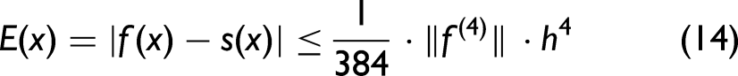
Another way to estimate the error bound
These estimated error limits are comparable to the error due to the numerical uncertainty in locating the centroid position of the calibration spectral lines, which is 0.0025 to 0.0125 nm, for SNRs of 250 and 50 respectively.
Conclusion
The process of pixel-to-wavelength calibration of a photosensor array spectrometer typically involves fitting a high-order polynomial to the calibration data or optimizing the parameters of an optical model of the spectrometer. A new method is proposed using cubic Hermite spline (CHS) interpolation with the calibration points treated as fixed points and as the nodes of the spline interpolation. When the interpolating functions are expressed in terms of Hermite basis functions, the calibration points (the reference wavelengths and their pixel locations) and the slopes at those points explicitly appear in the coefficients of the Hermite functions. The slopes or wavelength linear dispersion are derived from the grating equation and the physical model of the optical system of the spectrometer. The CHS interpolation calibration functions appear in closed form, eliminating the need for intermediate computations,— such as polynomial regression for polynomial fitting, or least-squares optimization for parametrized optical models,— to determine the calibration curve. This calibration method is especially advantageous for spectrometer systems with limited computing resources.
The calibration method was tested using a compact spectrometer system using a flat-field concave grating as the single optical element. The residual error (defined as deviations from the reference values of the calibration spectral lines) is zero by definition for the CHS interpolation, and the estimated interpolation errors are less than the residual error of a polynomial fit. The CHS interpolation, which uses slopes calculated from the optical model, yields the lowest interpolation errors that are comparable to the physical uncertainty of the spectral line peak location due to the optical resolution of the spectrometer system.
Footnotes
Acknowledgments
The authors acknowledge and thank Professor Dr. Gil Nonato Santos, iNano Laboratory, Center for Natural Science and Environmental Research, and Department of Physics, College of Science, De La Salle University, Manila, Philippines, for providing space and facilities at the iNano Laboratory.
We also thank the reviewers for their valuable insights and comments.
Funding
The authors received no financial support for the research, authorship and publication of this article.
Declaration of Conflicting Interests
The authors declared no potential conflicts of interest with respect to the research, authorship, and/or publication of this article.