Sage Journals: Discover world-class research

Abstract

The use of dispersive near-infrared (NIR) absorption spectroscopy in real-time fuel property measurement is a promising approach for enhancing engine performance. Such sensing, coupled with appropriate controls, may broaden the range of viable fuels available for use in compression ignition (CI) engines. An important fuel property for CI engines is the cetane number/derived cetane number (CN/DCN). This study builds upon recent work focusing on employing vibrational spectroscopy for determining CN/DCN for real-time on-board sensing. The NIR region, measured with moderate resolution, has some variability in the combination bands from which models can be generated for the prediction of fuel properties, at least for fuels similar to current jet fuels. Sensing in this region is relatively low-cost and robust compared with other spectral regions and schemes. Machine learning (ML) models to predict DCN from NIR spectral data are described. These models can address some of the challenges associated with on-board deployment, including sensing spectral range/resolution shifts and baseline shifts. The resolution and ranges of measurements on a sensor can be different than those on analytical devices used to collect the training set and generate the models. Two ML model approaches, one based on imputation and the other based on ensemble models, are evaluated to tackle that problem. The results indicate that the ensemble model is capable of accurate predictions achieving a coefficient of determination (R² score) above 0.86 when evaluated across various resolutions, i.e., 12 nm, 10 nm, and 2 cm^–1, and achieved an average R² score of 0.857 when evaluated on varying spectral range.

Graphical abstract

This is a visual representation of the abstract.

Keywords

Cetane number fuel sensing spectral imputation ensemble models dispersive near-infrared fuel sensor

Introduction

Spectroscopic fuel sensors have been prototyped and tested to provide real-time measurements of fuel properties,^1,2 particularly the derived cetane number of jet fuels. The cetane number/derived cetane number (CN/DCN) is an important fuel property for compression ignition (CI) engines. It is not specified for jet fuel certification,³ and thus jet fuels have some variability in DCN. The CN/DCN is associated with the ignition delay time (IDT), which is defined as the time interval from the start of injection (SOI) to the start of combustion (SOC). This time delay measures the period until combustion begins under elevated temperature and pressure conditions. Cetane numbers lower than 40 can result in engine misfires due to long IDTs.

Beyond the current variability in conventional fuels, any integration of alternative fuels (for now blended with conventional fuels) will affect both the chemical composition and key properties of the fuel supply.⁴ Due to various production methods and lack of specification for DCN, fuel blends can have significant variance in DCN.^1,5–7 This potential for variability in DCN, coupled with its critical role in CI engine performance, has increased the need to monitor fuel properties both before and during operation. DCN is an imperfect property for aviation CI engines, but CN/DCN is a well-established fuel property with standardized testing methods (ASTM D613, D6890), allowing for reliable and consistent measurement across fuels and is therefore widely available. With respect to other engine configurations, DCN significantly influences gas turbine operation, particularly in parameters like lean blowout (LBO) limits, which are essential for ensuring stable and efficient combustion.^8,9 While IDT and LBO are more directly tied to combustion performance, they are dependent on engine-specific factors such as injection strategy and operating conditions, making them less practical for broad characterization of fuels and blends. In contrast, the standardized processes for determining CN/DCN involves the use of equipment like cooperative fuel research (CFR) engines, ignition quality testers (IQTs), or fuel ignition testers (FITs).^9,10 Unfortunately, these conventional apparatuses are large, heavy, and have high fuel consumption requirements, making them unsuitable for on-board applications. Therefore, spectroscopic fuel sensors incorporated into an engine with adaptive control and ignition enhancement can enable CI engines to operate on a wider range of fuels and may lead to efficiency improvements.

Studies have shown that fuel properties can be correlated with the infrared (IR) absorption spectra of fuels with the use of machine learning (ML).^11–13 Jet fuels are dominated by hydrocarbons,^4,6 which exhibit important absorbance bands in the mid-IR region (1800–6250 nm) corresponding to strong symmetric and asymmetric CH₂ and CH₃ stretches. Further into the IR (6250–25 000 nm), also known as the fingerprint region, several bands from the vibrational bending of functional groups provide strong and unique features making the spectral region ideal for property determination.¹³ Dalmiya investigated the prediction of DCN obtaining a coefficient of determination (R² score) of 0.95 and 0.94 using two different spectral regions (4000–12 500 nm and 4167–12 500 nm respectively).¹³ Al Ibrahim and Farooq demonstrated the prediction of DCN and research/motored octane numbers (RON/MON) using simulated IR data of hydrocarbon blends, diesel, and gasoline blends.^14,15

Although distinct bands are present in the mid to far IR range, weak first and second C–H overtone and C–H combination vibrational mode absorbances are also present in the NIR (shown in Figure 1). Although the bands are weak, subtle differences are present and can be used for property prediction.^16–18 Traditionally, more spectral data would aid in achieving more accurate predictions, but Brouillette et al. observed the first C–H overtone region had a negative impact on predictive capabilities for density, cetane index, viscosity, aromatic content, and flash point and relied on the second C–H overtone and C–H combination band for property predictions. To enhance the variations measured in those bands and increase the signal-to-noise ratio, a longer pathlength was used.¹⁶

Figure 1.

Absorbance of liquid jet fuels collected using a 1 mm pathlength.

Additional studies have been conducted where the first C–H overtone region was neglected, and these studies focused on spectral regions encompassing the second C–H overtone and C–H combination band. Lysaght et al. used a NIR spectroscopic method on 33 samples of JP-4 and ML models to predict the freezing point and volume percentage of aromatics and saturates present in fuel samples.¹⁹ The spectral range of interest was 700–1500 nm, and models achieved an R² of 0.85 and a standard error of 3.92 °C.¹⁹ Xing et al. developed a method for estimating the kinematic viscosity and acidity of aviation kerosene using ML models trained on spectra collected within a range of 700–1100 nm. Predictions were made using a calibration model using partial least squares (PLS) regression with an R² of 0.9582 and a standard error of fit of 0.012 mm²/s for kinematic viscosity.^20,21 A study by Cooper et al. used a handheld NIR analyzer to collect jet fuel spectra to predict fuel properties such as American Petroleum Institute (API) gravity, percent volume aromatics, cetane index, density, freezing point, percent saturates, flashpoint, 10%50%90% recovered distillation temperatures, and hydrogen content.¹⁷ The spectra of JP-8, Jet A-1, and Jet A fuels were collected using a FUELex NIR handheld fuel analyzer with a fiber-optic dip probe, and the spectral range of interest was 880–1570 nm. Among the properties, the API index showed a high R² score of 0.99, and the recovered distillation temperature (90%) showed the lowest R² score of 0.62. Although calibration models (i.e., PLS) have been used for correlating spectra to properties, these types of models are limited to the range of values present in the training data and struggle to generalize beyond it.

In a previous work, a spectrum to DCN ML model was deployed on a dispersive NIR fuel sensor (operating on a 10 mm pathlength) to evaluate the capability of real-time fuel property determination.² In that work, the dispersive NIR fuel sensor deployed a model that had a R² score of 0.83, mean percentage error (MPE) of 5.63% and predicted 84% of test set samples within ±10% error.² Although the dispersive NIR sensor performed well in a demonstration of a fuel supply switch,² the model deployed in that sensor required a perfect matching of range and resolution across spectral elements, i.e., the model predictors form a bijection with the pixels of the spectrometer, and the models were trained exactly for those pixel predictors. In that demonstration, there were 123-pixels spanning the spectral range of 952–1645 nm. Such a model is thought to have limitations because it is not robust to wavelength calibration changes on the order of pixels. It is unreasonable to expect that mass-produced sensors with dispersive elements would have the same calibration down to the pixel, let alone retain calibration in that manner, robust to temperature and vibration fluctuations.¹ This issue is relevant in laboratory settings and would be expected to be worse, even for a ruggedized on-board fuel sensor.

This limitation can be mitigated by implementing on-board wavelength calibration, e.g., by using calibration standards. The new wavelength assignments might result in different spectral range and resolution that do not match the input predictors for the deployed ML model.²² Even if a pixel-to-pixel mapping strategy could be reliably implemented, perhaps with orthogonal signal correction,²³ it is unclear how the edges of the spectra should be handled. One approach would be to model on a narrower spectral range than the nominal calibration range, permitting minor drifts. Such methods are characterized as deletion methods,²² but they can leave off potentially important regions.

This problem motivates the need to develop models that are capable of operating on slightly varying spectral ranges (potentially even large shifts caused by on-board deployment) and resolutions to accommodate wavelength recalibrations in sensors. Achieving this goal will also enable the ML models to easily transfer among both different units of nominally identical sensors and different fuel sensor models that may employ varying spectrometers with differing spectral ranges and resolutions. Two approaches are formulated. The first approach takes advantage of imputation techniques to develop a robust model. Imputation techniques allow for missing data to be estimated or filled in by techniques such as interpolation/extrapolation, regression imputation, constant (single-value) imputation, k-nearest neighbors (KNN), mean imputation, etc.²⁴ The second approach uses an ensemble ML model strategy to develop a robust model framework. Ensemble ML involves training numerous base models on subsets of the dataset and combining their predictions to produce a meta-model that provides the final prediction.²⁵ This approach involves base models trained using different types of regression models such as linear regression, multilayer perceptron (MLP), support vector regression (SVR), and lasso regression. By employing a decision template, aggregating the predictions of these base models to develop meta models, the ensemble method can enable accurate predictive capabilities over varying predictors.^25–27

In this work, the imputation and ensemble model approaches are employed to generate ML models capable of predicting the DCN of jet fuels and near jet fuels based on absorption signals over spectral ranges between 950–1650 nm. The experimental methods and the description of the dataset will be discussed in the following section. Next, the methodologies employed to train and evaluate the models are discussed followed by an evaluation of the developed models on varying spectral resolutions and regions. These robust models contribute to enabling a dispersive NIR fuel sensor to operate for on-board sensing.

Experimental

Materials and Methods

Six spectrometers were used to obtain absorption measurements for the dataset. Table S1 (Supplemental Material) shows details of the setups used for each spectrometer. A Thermo Fisher Scientific Nicolet iS50 Fourier transform near-infrared (FT-NIR) spectrometer was used to collect data from 833 to 2500 nm at 2.0 cm^–1 resolution. Four Ocean Insight Flame-NIR + spectrometers were used to collect data from a nominal range of 900–1700 nm with a resolution of 10 nm. The Flame-NIR spectrometers are fiber coupled (QP600-1-VIS-NIR from Ocean Insight, 600 µm core diameter with a numerical aperture of 0.22) to 10 mL quartz cuvettes (LAB4US) with path lengths of 10 mm. The cuvettes are placed within a temperature-controlled cuvette holder (Quantum Northwest) and held at 10 °C. The light source is a fiber coupled IR stabilized source (Thorlabs). Finally, an Ibsen Photonics Pebble NIR spectrometer was used to collect data from 946–1700 nm at a resolution of 12 nm. This setup used the same cuvettes and light source as the Flame-NIR + .

An IQT at the University of Illinois Chicago was used to evaluate the DCN of all the mixtures and real fuels in the dataset. Each sample was tested three times under the same conditions in compliance with ASTM 6890 standards. The three test runs for each sample were then averaged to determine the final DCN. The DCNs of this dataset have been published recently by Sheyyab et al.²⁸

Dataset

Developing a spectroscopic fuel property sensor capable of predicting the diverse physiochemical properties of fuels requires a dataset that is representative of the physiochemical variability present in fuels. Training ML models on every available fuel is impractical and would introduce bias toward the fuels present within the training dataset. To generate a comprehensive dataset, Mehta et al. used approximately 17 real fuels and complex CN fuel surrogates provided by the Combat Capabilities Development Command (DEVCOM) Army Research Laboratory (ARL).²⁹ The study entailed the use of two-dimensional gas chromatography coupled with flame ionization detection and time of flight-mass spectrometry analysis to characterize the fuels. The components were classified into family/size-based categories, and a chemical functional group fragmenter was applied to suggest the ranges of UNIFAC chemical functional groups present in the fuels under study. Using these UNIFAC functional group ranges, the DCN ranges, molecular weight ranges (MWs) of these real fuels, along with a selection of pure hydrocarbons, Sheyyab et al.²⁸ generated a set of 79 mixtures of up to four components, with some coming from a functional group optimizer and some otherwise selected. The mixtures encompass the range of UNIFAC chemical functional groups, DCNs, and MWs of real jet fuels. The performance of the model developed by this dataset assumes the dataset is representative of the population of both current and prospective aviation fuels, including those derived from non-petrochemical sources. There is some uncertainty in this assumption, but current fuels have some compositional and chemical family similarities, so it is reasonable to expect future aviation fuels passing specification will have compositional and chemical family similarities.²⁹ Table I shows the training and testing dataset used for this work. Only 78 mixtures of the Sheyyab et al.²⁸ mixtures were used in this work. One two-component mixture (P200029 comprised of undecane and cumene) was unavailable. Further details of the specific mixtures are available in the supplemental material. It should be noted that the training set in this work contains spectral measurements obtained using the FT-NIR and Flame-NIR + spectrometers (630 measured absorbance spectra). The FT-NIR absorbance data was collected at a 1 mm pathlength and was then scaled to a 10 mm pathlength using simple multiplication. Additionally, three test sets comprised of the same fuels and fuel blends described in Table I were used in this work to evaluate the models. The three test sets are distinguished by the spectral resolution at which the test set data was collected. The three test sets are the Flame-NIR+, Ibsen Pebble, and FT-NIR test sets (collected at 10 nm, 12 nm, and 2 cm^–1 resolutions, respectively). The use of three different test sets enables evaluating the developed ML models on varying spectral resolutions, and each test set is also evaluated on varying spectral ranges. The Flame-NIR + test set with a spectral range of 950–1650 nm is used as the test benchmark for this work.

Table I.

Training and testing dataset used in this work.

Training set		Testing set
Name, description, or POSF (as applicable)	DCN	Name, description, or POSF (as applicable)	DCN
78 mixtures made using 23 neat hydrocarbons ARL-CN30 ARL-CN35 ARL-CN40 ARL-CN45 ARL-CN50 ARL-CN55 F-24 ATJ–POSF11498	15– 105 34.7 36.7 41.9 49.7 55.1 59.5 46.6 15.9	JetA1–POSF10264 JetA2–POSF10325 JetA3–POSF10289 (JP5) 50/50 wt% ARL–CN35/CN55 50/50 wt% ARL–CN35/CN45 50/50 wt% ARL–CN30/CN50 50/50 wt% ARL–CN45/CN55 50/50 wt% ARL–CN35/CN40 50/50 wt% F-24/ATJ 30/70 wt% F-24/ATJ 70/30 wt% F-24/ATJ 20/80 wt% F-24/ATJ 40/60 wt% F-24/ATJ 60/40 wt% F-24/ATJ 80/20 wt% F-24/ATJ	49.3 49.0 40.2 49.6 43.0 45.1 54.7 39.8 34.6 29.6 39.5 28.3 34.0 39.1 43.4

Preprocessing Methods

Prior to training any machine learning models, the collected absorbances are preprocessed using custom routines developed in Python. Figure S1 (Supplemental Material) outlines the preprocessing steps, where the required input is a running mean baseline corrected absorption spectra. Equations 1 and 2 are used to perform this initial baseline correction.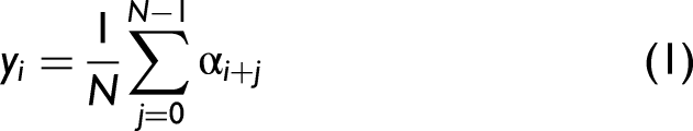

y_{i} = \frac{1}{N} \sum_{j = 0}^{N - 1} α_{i + j}

(1)

{\overset{´}{α}}_{i} = α_{i} - min (y)

(2)

in which

α_{i}

represents the absorbance at wavelength measured at pixel, i, N is the window size, and

y_{i}

is the moving average. The minimum value of the moving average is used to subtract the baseline noise from the original absorbance data, resulting in a baseline corrected absorbance denoted by

α_{i}^{'}

in Eq. 2. This constant running mean baseline correction is applied on each measured absorbance spectrum in the dataset.

The spectral preprocessing steps enable measured spectral data (wavelengths and absorbances) of varying spectral ranges, resolution, and number of datapoints to be uniformly represented as model predictors. To achieve a uniformly represented spectral dataset, the spectral range of interest (ROI) and the desired number of equally spaced wavelength model predictors within the ROI are selected. For this work, a ROI of 950–1650 nm with 175 datapoints is used. Using the ROI and desired number of model predictors, an array of uniformly spaced wavelengths is created; in this work, the wavelength spacing of the model predictors is about 4.02 nm.

It is important to consider how each absorbance data point accounts for the absorbances measured around the target predictor wavelength. In this work an additional spacing value of ±8 nm is used. This spacing value determines the size of the binning window to ensure the preprocessing technique can adequately include relevant features without losing important details due to measurement limitations. Measurement limitations arise from the spectrometer's resolution and the density of data points collected.

The steps outlined under spectral preprocessing in Figure S1 (Supplemental Material) are performed for each measured absorbance spectrum allowing each spectrum to be uniformly represented as model predictors. Figures 2a and b show the measured absorbance of F-24 collected using different spectrometers (measurements from FT-NIR are represented by green circles and from the Flame-NIR + are denoted by red circles). Overlayed on top of those spectra are the uniformly spaced wavelength model predictors (represented by yellow circles). The size of the binning window is determined by the model predictor ± the spacing value. Illustrated in Figure 2a by an orange circle at 1219.5 nm, a model predictor, and all measured spectral data within the model predictor ± spacing value (i.e., 1219.5 ± 8 nm) are then binned for that model predictor. The binned datapoints (wavelength and absorbances) are then used to perform an interpolation to a single model predictor. If 4 + datapoints are binned, a cubic interpolation will be performed using the binned spectral data to determine the absorbance at the predictor wavelength; however, if only two or three datapoints are binned, a linear interpolation–extrapolation is performed. Lastly, if 0 or 1 datapoint is binned, the absorbance at the predictor wavelength will be not a number (NaN). This process is iterated for each predictor in the array of uniformly spaced wavelength model predictors, in this case, 175 times per spectrum. Upon binning, the absorbance model predictors are baseline corrected an additional time. A second-degree polynomial baseline correction is performed using pybaselines modified polynomial (ModPoly) function.^30,31 This function effectively isolates the true absorbance signal by removing baseline distortions, enhancing the accuracy of the data. Figure 2c shows the model predictors of F-24 after the spectra are preprocessed, where the green spectrum was collected on the FT-NIR and red spectrum was collected using a Flame-NIR +. This preprocessing methodology is utilized for the training and testing of ML models. An alternative preprocessing scheme was investigated; however, it was deemed to be less effective therefore was not used. Additional information regarding the alternative preprocessing scheme can be found in the Supplemental Material.

Figure 2.

Absorbance spectra of F-24 fuel measured using (a) a FT-NIR with a resolution of 2 cm⁻¹ and (b) a Flame NIR spectrometer with a resolution of 10 nm. Yellow markers indicate the specific wavelengths (model predictors) used as inputs to the ML model(s). The inset in subfigure (a) illustrates how the absorbance value corresponding to a model predictor was selected using the binning window approach (described in Figure S1). Figure 2c shows the 175 preprocessed model predictors from both measured spectra after baseline correction.

Spectral Imputation Approach

As previously reported, Method 1 employs imputation techniques to create a robust spectral model. Interpolation and extrapolation imputation, while commonly used in ML applications,^32,33 may not be suitable for spectral models. An inaccurate interpolation/extrapolation may alter the presence/absence of spectral features, which can negatively impact model performance. Alternatives like regression, KNN, and mean imputation have been explored in ML studies;^34–36 however, these methods are dependent on the dataset used. This dependence on the dataset can introduce bias when handling missing spectral data, as the imputation technique will rely on the available dataset to fill in missing spectral data.^37,38

To address these issues and reduce any possibility of bias, single-value (constant) imputation is used. Conventionally, single-value imputation is considered to be one of the weaker imputation techniques, as this approach assumes all missing values to be the same value, likely causing considerable distortions in the dataset.³⁹ However, by intentionally introducing a constant value to represent missing spectral data within the training dataset, a model may become more familiar with missing spectral data and better equipped to handle such encounters during deployment. The schematic of the imputation model is shown in Figure S4 (Supplemental Material). In this work, all missing absorbance values are replaced with constant value of 0.

Augmentation of the training data set is used to introduce absorbance measurements with missing spectral data. The augmentation is completed by creating input predictors within the training dataset where certain spectral ranges are intentionally left unmeasured. This is done by defining spectral subregions within the desired range of interest of the model. For this work, 105 spectral subregion combinations are chosen, covering the range of 950 to 1650 nm. These combinations include 14 combinations of 50 nm increments with no overlap, 13 combinations of 100 nm increments with 50 nm overlap, 12 combinations of 150 nm increments with 50 nm overlap, 11 combinations of 200 nm increments with 50 nm overlap, 10 combinations of 250 nm increments with 50 nm overlap, nine combinations of 300 nm increments with 50 nm overlap. This pattern continues, decreasing by one combination for each additional 50 nm increment, until reaching a single combination for the increment of 700 nm with no overlap. The definitions of these 105 subregions are included in the supplemental information. Using the described spectral subregion combinations, the experimental training model predictors within the spectral subregion are used, and the remaining predictors are set to 0. Figure 3a shows some spectral subregions from a preprocessed absorbance of F-24, and Figures 3b–d are examples of augmented data with missing spectral data. This is done for the entire training dataset, resulting in a missing data augmented training dataset of 66 150 absorbance spectra (with varying spectral data and imputed missing data with a constant value of 0).

Figure 3.

(a) Spectral subregions in the data augmentation of the imputation method. (b) 1400–1450 nm, (c) 1350–1600 nm, (d) 1000–1250 nm, and (e) 950–1650 nm.

Once the augmentation of missing spectra data is completed, an additional augmentation is performed to account for spectral noise. This involves generating noise specifically for spectral measurements (non-zero data). To do this, an array of noise is created, where random noise with a standard deviation of 0.005 is added to the original spectral measurement. After adding the noise, the modified absorbance measurement is added into the training dataset. As a result of this process, the final training dataset is twice the size of the original one, as the original data is maintained and the data with augmented noise is added to the dataset. At this point, the dataset is split for training and testing of a ML model. The training process entails hyperparameter optimization, which varies depending on the models employed. Further details of hyperparameter optimization in this work are discussed in the Models and Hyperparameter Optimization section of this manuscript. Once the model is trained, the model is evaluated on the test benchmark, as well as varying spectral ranges and resolutions to understand the capabilities and limitations of the spectral imputation model development approach.

Ensemble Models Approach

Method 2 leverages ensemble learning by using bootstrap aggregation (bagging) and stacking techniques coupled with a decision template classifier.^24–26 Ensemble learning is an ML approach where multiple base models are combined to enhance predictive performance. Typically, ensemble learning involves training base models on different features or predictors and using stacking techniques to combine their predictions for a final output.²⁵ In this method, instead of training base models on different predictors, bootstrap aggregation is used to create subsets of the predictors for training. Specifically, the spectral measurement is divided into smaller spectral subsets, and base models are trained on these narrow spectral regions. This approach varies from feature selection as feature selection aims to optimize the spectral subsets/features required for accurate predictive capabilities and will only rely on the selected features for predictive capabilities.¹² Ensemble learning with bootstrap aggregation coupled with a decision template will utilize all available spectral subsets to perform predictions using base models and will focus on aggregating the base model predictions using stacking techniques to generate a final prediction.^25,26

As one of the main objectives of this work is to enable predictive capabilities over varying spectral ranges, a decision template classification is integrated into this approach. The decision template ensures that predictive capabilities are maintained even when some base models are unable to provide predictions due to incomplete spectral coverage. By using the decision template, the model can reliably aggregate predictions from the available base models, ensuring consistent performance despite variations in measured spectral data.

The methodology is shown in Figure S5 (Supplemental Material). The first step after the spectral preprocessing step is to train base models on subsets of the spectral data. With 950–1650 nm spanning the entire spectral range of this work, 14 base models with 50 nm subregions are used (see Figure 4), where the spectral subregions do not overlap. Each base model is referred to as a letter as indicated in Figure 4. The spectral subregion training data is augmented to account for spectral noise, as described previously, followed by training the base models using hyperparameter optimization, as discussed in the Models and Hyperparameter Optimization section of this manuscript.

Figure 4.

Defined spectral subregions for base model training overlayed on absorbance spectra of F-24.

Upon training the base models, the next step aggregates the base model predictions for a final DCN prediction. In this work, two approaches are used to aggregate the base models, averaging and meta models. The averaging approach computes the sum of the base model predictions and divides it by the number of base models used. This approach does not require training. The meta model approach requires models to be trained for each possible scenario of which base models were able to provide a prediction. The training data for these meta models are the DCN values predicted by the base models during the training process. The meta model spectral ranges consist of 13 meta models that aggregate predictions from two base models (100 nm of spectral data), 12 meta models that aggregate three base models (150 nm of spectral data), 11 meta models that aggregate four base models (200 nm of spectral data), 10 meta models that aggregate five base models (250 nm of spectral data), nine meta models that aggregate six base models (300 nm of spectral data). This pattern continues, decreasing by one meta model for each additional 50 nm increment, until reaching a single meta model to aggregate 14 base models (700 nm of spectral data). This results in a total of 91 meta models, each identified by the first and last base models in use (e.g., a meta model using all 14 base models is referred to as meta model A-N). These details are included in the supplemental information.

To determine the best aggregation approach for each spectral subregion, the meta models are evaluated using different stacking techniques, including linear regression, lasso regression, and SVR, with hyperparameter optimization.

The integration of a decision template allows for flexibility in choosing the most effective aggregation/stacking technique when aggregating various base model combinations (various spectral ranges). For example, while an SVR meta model might be optimal when all 14 base models are used, it may not be the best choice when only seven base models are available. This flexibility is a key advantage of the ensemble approach, as it allows for the use of various models without being restricted to a single aggregation/stacking technique. The decision template is formulated by evaluating the R² score for each spectral range meta model when using the respective spectral range. Completion of this evaluation results in a model framework comprised of 105 models, where 14 of them are the base models, 90 meta models that aggregate various subregion combinations and one meta model that aggregates entire spectral region (950–1650 nm).

Models and Hyperparameter Optimization

In this study, three ML models are employed using Scikit-Learn: linear regression, lasso regression, and support vector regression (SVR).⁴⁰ Linear regression is a fundamental model that assumes a linear relationship between input features and the target variable, making it a widely used baseline model in regression tasks. lasso regression builds on linear regression models by introducing regularization, which helps manage model complexity and improve generalization. SVR provides a more flexible method capable of modeling both linear and non-linear relationships, allowing for a broader exploration of the data. Together, these models represent a spectrum of approaches, from basic linear methods to more versatile non-linear modeling techniques. To achieve robust ML models, hyperparameter optimization is completed using Scikit Learn's GridSearchCV function.⁴⁰ The hyperparameters used in the optimization of a model will vary depending on the model employed. Table S2 (Supplemental Material) shows the hyperparameters used in this work for their respective model.

As the simplest model, linear regression only has one parameter to optimize: the fit intercept. The fit intercept parameter determines whether an intercept should be computed for the model. Including an intercept can introduce bias, but it is often useful if the data are not grouped/centered. Lasso regression models are optimized using three key parameters: fit intercept, alpha (α), and selection. α controls the regularization strength in Lasso models. Regularization penalizes large coefficients to help prevent overfitting. A large α value increases regularization, shrinking the coefficients closer to zero. The α values typically range from 10^–4 to 10. The selection parameter dictates the strategy used to minimize the cost function. Two options are available: cyclic and random. Cyclic coordinates an iteration algorithm over each feature in the training data one at a time and updates the coefficients after each iteration. The cyclic strategy is more reproducible but slower for large datasets with many features. On the other hand, the random strategy is much quicker, but the resulting model may vary due to the randomness.

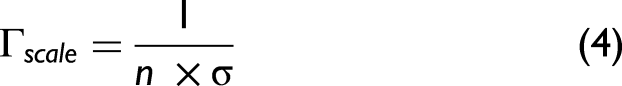
There are four critical hyperparameters that will dictate the capabilities of an SVR model. Those parameters are the kernel, regularization parameter (C), epsilon (ɛ), and gamma (Γ). The kernel is a mathematical function that allows the model to handle more complex relationships in the data by mapping the input data into a different feature space. A linear kernel applies no transformation and directly works with the input features as they are. A polynomial kernel introduces polynomial combinations of the input features, allowing the model to capture polynomial relationships. The radial basis function (RBF) kernel calculates the similarity between data points based on their distance and applies a Gaussian transformation to create more complex decision boundaries. The choice of kernel depends on the nature of the data and the relationships that need to be modeled. The regularization parameter dictates the tradeoff between achieving low error on the training data and minimizing the norm weights. The regularization parameter helps prevent overfitting of the model. A small C value means the model is more tolerant to errors causing more regularization suggesting a underfitted model. On the other hand, a large C value allows for lower tolerance to errors potentially leading to overfitting. Typically, the regularization parameter is in the range of 10^–2 to 10⁴. Epsilon (ɛ) (usually ranging from 10^–3 to 1) defines the allowable tolerance where no penalty is given to errors. A larger epsilon results in larger tolerance to error, which may lead to underfitting. Gamma (Γ) defines the influence a single training data point has on the model. A small Γ value means each data point has a larger influence potentially resulting in underfitting. Gamma values can be manually defined or calculated by setting Γ equal to Auto or Scale. Auto utilizes Eq. 3, where n is the number of features, and is considered to be less effective than Scale as it will not account for the distribution of the training data. Scale computes the Γ value using Eq. 4, where n is the number of features and $σ$ the variance of the input features, accounting for the variance present in the training set. Typically, these Γ values range from 10^–4 to 1.

Γ_{a u t o} = \frac{1}{n}

(3)

Γ_{s c a l e} = \frac{1}{n \times σ}

(4)

The use of learning curves enables visualization and assessment of a model's performance as the training dataset size increases. By plotting the training and validation scores against the number of training samples, learning curves reveal trends that indicate whether the model is underfitting or overfitting. Underfitting occurs when both the training and validation scores remain low and close to one another, suggesting that the model lacks the complexity needed to capture the data's underlying structure. In contrast, overfitting is detected when the training score is high, but the validation score is low, indicating that the model has captured patterns specific to the training data but fails to capture broader trends effectively.

Varying both the training size and hyperparameters simultaneously provides a deeper understanding of how each parameter influences learning performance. For instance, in SVR models, hyperparameters such as kernel choice and regularization parameter (C) impact both model complexity and stability as more data is introduced. Analyzing learning curves with different parameter settings clarifies each parameter's role in controlling model flexibility, aiding in the identification of hyperparameter values that maintain consistent validation performance across training sizes. Figure S6, for example, shows learning curves for an SVR model with varying training sample sizes and regularization parameter values (C). Analyzing these learning curves indicates that a C value of 100 yields a suitable fit, as both the training and validation scores are high and close to one another, suggesting the model's capacity to capture the data trends accurately. As the C value continues to increase, the training score remains high, but the validation score decreases, indicating overfitting.

Generating learning curves across multiple hyperparameter settings helps determine the best values for each parameter; however, this process can be computationally expensive and labor-intensive, as it requires training the model on numerous data subsets and analyzing the curves to manually select the best hyperparameters. To streamline this process, a grid search is combined with 10-fold cross-validation. In this approach, the training data is divided into ten subsets. Each subset serves as a validation set once, while the remaining nine subsets are used for training. This procedure is repeated ten times, ensuring each subset of the data is used for validation. By averaging performance metrics across these ten iterations, cross-validation reduces sensitivity to any specific data partition. The grid search then identifies the combination of hyperparameters that yields the best average performance across all folds. After determining the optimal hyperparameters, the model is retrained using the entire training dataset with these values, resulting in a hyperparameter-optimized model.

Results and Discussion

Using the preprocessing techniques and model development approaches described above, an imputation approach ML model and an ensemble ML model framework (comprised of 14 base models and 91 meta models) are trained. Nonlinear models are generally more effective at correlating spectral features with fuel properties, particularly when the relationships involve complex interactions. Fuel properties are influenced by multiple molecular interactions, leading to nonlinear relationships. Accordingly, the imputation-based model and the 14 base models in the ensemble framework employ the SVR model, as linear models were found to be less effective at capturing these relationships. However, linear models are investigated for aggregating the predictions from the base models in the ensemble approach.

Each model development approach is assessed on training and testing metrics, such as coefficient of determination (R² score), mean absolute percentage error (MAPE), mean absolute error (MAE), mean squared error (MSE), percent of samples with +/–10% error, and percent of samples with +/–15% error. The R² score serves as an indicator of how well the input variance can predict the output variance. In the context of this work, how well the spectral features/data can predict the variance in the DCN (or any other fuel properties). R² scores values range from 0 to 1, with 1 indicating the model is fully capable of predicting the output variance. The MAPE measures the averaged absolute percentage error between the predicted and actual values. Ideally, an MAPE value near 0 is desired, indicating a small percent error between the predicted and actual values. MAE quantifies the average absolute difference between predicted and actual values. It describes how far off predictions are on average, excluding the direction of errors. MSE measures the average squared difference between predicted and actual values. MSE penalizes larger errors, unlike MAE, due to the squaring, making it more sensitive to outliers and large prediction errors. Ideally, both the MAE and MSE should be close to 0. These metrics can be used to evaluate the model on the training and testing set. The percentage of samples within +/–10% and 15% error are only used when evaluating the model on the test set. As mentioned earlier, the benchmark test set is collected using the Flame-NIR + at a 10 nm resolution over the spectral range of 950–1650 nm. After evaluating the two model approaches on benchmark test case, both models are compared and evaluated on varying spectral ranges on 10 nm resolution spectral data and varying spectral ranges on different resolutions (12 nm and 2 cm^–1 resolution, collected using the Ibsen Pebble and FT-NIR, respectively).

Spectral Imputation Model and Performance

Using the methodologies discussed in the Preprocessing Methods, Spectral Imputation Approach, and Models and Hyperparameter Optimization sections of this manuscript and the training dataset described in Table I, an SVR imputation ML model was trained. The training data, represented by grey circles in Figure 5, achieved a training R² score of 0.831. This indicates that the model is able to correlate spectral features with the DCN effectively but imperfectly. In Figure 5, there are noticeable clusters of predicted DCN values that are vertically aligned at measured DCN values of approximately 90 and 105. The only sample in the training dataset (as outlined in Table II) with a DCN close to 90 is tetradecane. However, Figure 5 shows multiple predictions around a DCN of 90, which is a result of the missing data spectral augmentation and spectral noise augmentation applied to the dataset. By introducing this variability during the training process, the model may be more capable of handling missing spectral data effectively and provide accurate predictions, regardless of the spectral range measured.

Figure 5.

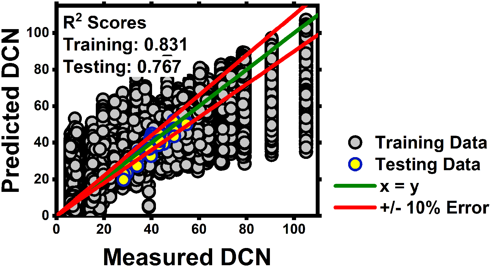
Training and testing of SVR imputation ML model.

Table II.

Imputation training and benchmark testing evaluation (950–1650 nm at 10 nm resolution).

Metrics	R² score	MAPE	MAE	MSE	Samples within ± 10% (%)	Samples within ± 15% (%)
Training	0.83	16.76	4.48	53.39	–	–
Testing	0.77	7.34	2.81	11.8	80.77	88.46

The trained SVR model is then evaluated on the benchmark test set (Flame-NIR + test set, 950–1650 nm at 10 nm resolution). The testing results are denoted by the yellow circles in Figure 5 and the evaluation metrics can be seen in Table II. These values suggest that the model is able to capture a significant portion of the variance in the data, with the R² score indicating that approximately 76% of the variation in DCN can be explained by the spectral features. The MAPE shows that the model's predictions are fairly accurate on average, deviating by about 7.3% from the true values. The MAE indicates that the model's predictions have an average error of 2.81 DCN, while the MSE of 11.8 highlights that most errors are relatively small, though a few larger deviations are present. Overall, the model performs slightly less than fair, indicating there is room for improvement, especially in minimizing the larger errors to enhance prediction accuracy. It can also be seen that only 80% of the test set samples were predicted within the ± 10% error criteria. Although this model has room for improvement when evaluated on the benchmark case, it is crucial to evaluate the models performance on varying spectral ranges and resolutions to understand the capabilities and limitations of the imputation methodology.

Ensemble Model and Performance

Using the methodologies discussed in the Preprocessing Methods, Spectral Imputation Approach, and Models and Hyperparameter Optimization sections of this manuscript and the training dataset described in Table I, fourteen SVR base models were trained. The training data for each SVR base model is represented by gray circles in Figure 6. The testing data points in Figure 6 refer to the base model predictions on the benchmark test set when using the respective 50 nm subregion spectral data for predictions. The predictions from these base models are not evaluated as final predictions, as these base model predictions need to be aggregated to obtain the final DCN prediction. However, it can be observed that certain subregions and base models provide decent predictions of DCN. Base models E, I, J, and K had intermediate to high training R² scores (>0.88), but subpar testing R² scores (>0.70). This suggests the corresponding spectral subregions contain spectral features that are highly correlated to the DCN but require additional information to explain the variance of DCN. It should be noted that the second C–H overtone typically falls in the range of 1150–1250 nm, but base model E has a spectral region of 1150–1200 nm, which covers about half of the second C–H overtone region. Base models I, J, and K span the range of 1350–1500 nm, which cover the exact range of the C–H combination band.

Figure 6.

Training and testing of SVR base models using ensemble model when using 50 nm spectral subset windows.

Four aggregation techniques are investigated (averaging, linear regression, lasso regression, and SVR meta models). Using the predicted DCN values of the training set as the training data of the meta models, three meta models are trained to aggregate the 14 base model predictions to obtain a final DCN prediction when using the spectral range of 950–1650 nm. The training data and metrics of the aggregation techniques can be seen in Figure 7 and Table III. It should be noted that the meta models all had a training R² score greater than 0.96, showing that the predicted DCN from each subregion are capable of being aggregated and combined for a final predicted DCN.

Figure 7.

Training and testing of meta models for aggregation of base models for 950–1650 nm spectral range.

Table III.

Ensemble aggregation training and benchmark testing evaluation (950–1650 nm at 10 nm resolution, aggregation of base models A-N).

Aggregation techniques	Metrics	R² score	MAPE	MAE	MSE	Samples within ± 10% (%)	Samples within ± 15% (%)
Averaging	Training	N/A	N/A	N/A	N/A	–	–
Averaging	Testing	0.71	6.19	2.80	14.65	75	92.3
Linear regression meta model	Training	0.96	7.08	2.47	11.78	–	–
Linear regression meta model	Testing	0.87	5.20	2.05	6.39	88.5	98.1
Lasso regression meta model	Training	0.96	7.13	2.48	11.88	–	–
Lasso regression meta model	Testing	0.88	5.02	2.00	6.30	88.5	96.2
SVR meta model	Training	0.99	3.12	1.15	3.23	–	–
SVR meta model	Testing	0.88	5.21	2.06	6.03	90.4	96.2

Not applicable: N/A

To evaluate the aggregation techniques on the spectral range of 950–1650 nm, the base models are first evaluated on their respective 50 nm of data on the benchmark test set. The yellow data points in each subplot from Figure 6 serve as the 14 predictors for the four aggregation techniques. The predicted DCNs of these 14 base models are then aggregated and compared to evaluate the best aggregation technique for the spectral range of 950–1650 nm. The averaging technique, being the simplest method, designates no importance to any particular base model treating them all equally as important. This aggregation technique obtained the worst R² score of 0.71 and highest MAPE, MAE, and MSE values, suggesting the averaging technique does not do a sufficient job in explaining the variance in predicted DCN values. Linear and lasso regression techniques performed extremely similarly as both approaches involve using the weighted average. This suggests that the variance of DCN in each subregion is linearly correlated to the true DCN of the fuel. It is noteworthy that the linear models performed similarly to the nonlinear SVR aggregation technique. The SVR stacking technique is the best performing approach as it obtained the highest R² score of 0.88 when evaluated on the benchmark test case. While the SVR meta model A-N does not have the lowest MAPE and MAE values, it does have the lowest MSE suggesting the SVR aggregation technique is able to provide final DCN values with less erroneous/outlier predictions. For instance, when tested on JetA3–POSF10289 (JP5), the Linear and lasso regression meta models exhibited average DCN errors of 4.52 and 4.09 DCN, respectively. Whereas the SVR meta-model demonstrated an average DCN error of 2.53 DCN.

Comparison of Models for Different Ranges and Resolutions

Using the imputation model and the ensemble model framework comprised of 105 models, a performance comparison is completed to understand the limitations and capabilities of both approaches when evaluated on varying spectral resolutions and ranges. The comparison of the imputation model and ensemble models framework can be seen in Figure 8, where six scenarios are presented.

Figure 8.

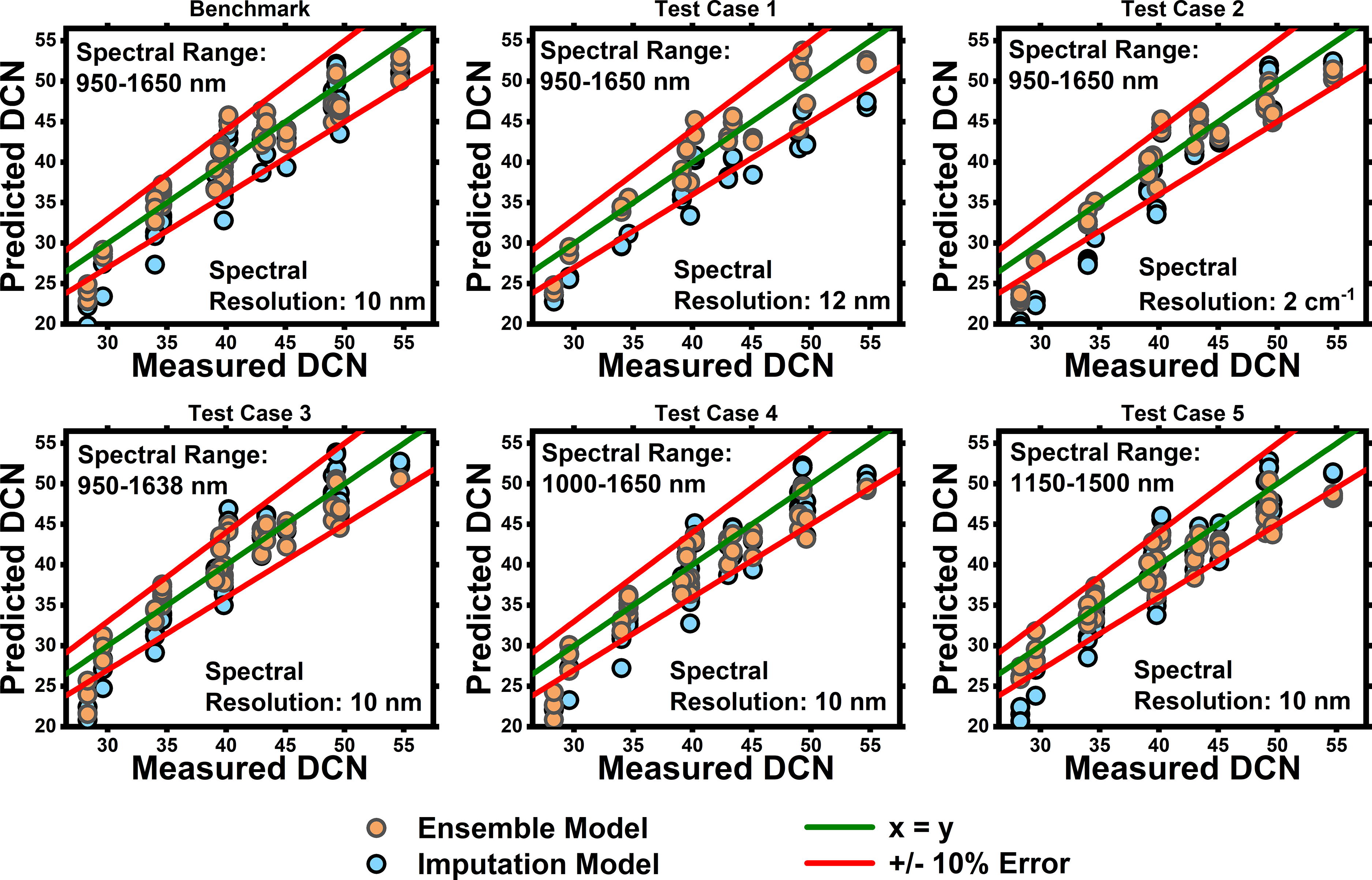
Comparison of imputation and ensemble model development approach on varying spectral ranges and resolutions.

The benchmark test case (as described in the previous sections) employs the Flame-NIR + test set, covering the spectral range of 950–1650 nm at a 10 nm resolution. As shown in Table IV, the ensemble modeling approach consistently outperforms the imputation model across all metrics. The ensemble model achieves an R² score of 0.88, compared to the imputation model's 0.77, and also has a superior performance in terms of MAE, MAPE, and other metrics presented. Notably, the ensemble model is capable of predicting 90.4% of samples within ±10% error, compared to 80.8% for the imputation model.

Table IV.

Model development approach comparison on varying spectral ranges and resolutions.

Test case	Approach	R² score	MAPE	MAE	MSE	Samples within ± 10% (%)	Samples within ± 15% (%)
Benchmark 950–1650 nm 10 nm resolution	Imputation	0.77	7.34	2.81	11.8	80.8	88.5
Benchmark 950–1650 nm 10 nm resolution	Ensemble	0.88	5.21	2.06	6.03	90.4	96.2
Test Case 1: 950–1650 nm 12 nm resolution	Imputation	0.52	10.9	4.51	25.2	38.7	83.9
Test Case 1: 950–1650 nm 12 nm resolution	Ensemble	0.87	5.35	2.22	6.84	87.1	96.8
Test Case 2: 950–1650 nm 2 cm^–1 resolution	Imputation	0.64	10.1	3.64	19.1	70.0	74.5
Test Case 2: 950–1650 nm 2 cm^–1 resolution	Ensemble	0.86	5.79	2.26	7.42	87.2	93.6
Test Case 3: 950–1638 nm 10 nm resolution	Imputation	0.81	6.43	2.42	9.49	82.7	90.4
Test Case 3: 950–1638 nm 10 nm resolution	Ensemble	0.87	5.14	2.03	6.36	88.5	96.2
Test Case 4: 1000–1650 nm 10 nm resolution	Imputation	0.76	7.43	2.84	12.0	80.8	88.5
Test Case 4: 1000–1650 nm 10 nm resolution	Ensemble	0.83	5.71	2.28	8.45	90.4	96.2
Test Case 5: 1150–1500 nm 10 nm resolution	Imputation	0.77	7.37	2.82	11.5	76.9	88.5
Test Case 5: 1150–1500 nm 10 nm resolution	Ensemble	0.84	5.25	2.23	7.88	86.5	100

For Test Case 1, the Pebble test set at a resolution of 12 nm is used, and both models see a decline in performance relative to the benchmark performance. However, the imputation model experiences a much more significant drop, with its R² score falling to 0.52. Meanwhile, the ensemble model shows greater resilience and maintains an R² score of 0.87. This is particularly noteworthy given that the same ensemble SVR meta-model A-N is used in both the benchmark case and Test Case 1. Since the spectral range (950–1650 nm) remains unchanged, the same base models needed to be aggregated within the ensemble framework, hence showing the ensemble model's capability of predictions on a different resolution.

Test Case 2 uses the FT-NIR test set at a high spectral resolution of 2 cm^–1, the performance gap persists. The imputation model improves slightly over Test Case 1 with an R² score of 0.64 but continues to lag behind the ensemble model's R² score of 0.86. The ensemble model continues to use SVR meta model A-N for this test case. Considering that 2 cm^–1 resolution data is used in the training data set, it can be observed that the imputation model performs better on Test Case 2 than Test Case 1. However, this was not true for the ensemble model as it performed similarly (∼0.86 R² score) when compared to the evaluation of 12 nm resolution data. This can likely be attributed to the fact that the imputation model is more sensitive to spectral resolution. The process of augmenting missing spectral data may have caused the imputation model to focus on handling varying amounts of missing data rather than accurately capturing the variations in absorbances (associated to varying resolution measurements) at each wavelength predictor. In contrast, the ensemble approach allowed each base model to capture the variance in absorbances within smaller subregions, and the final predictions are then aggregated, which may have made it more robust to changes in resolution.

In the Test Case 3 scenario, the spectral range is reduced from 950–1650 nm to 950–1638 nm, using the Flame-NIR + test set at a resolution of 10 nm. This test aims to mimic a situation where a slight shift towards the lower wavelengths is present. Despite the slight reduction in the spectral range, the performance of both models remains relatively stable when compared to the benchmark, in fact the imputation model performs better on the reduced range compared to the benchmark spectral range, indicating spectral data past 1638 nm does not aid in improving predictive capabilities. The imputation model achieves an R² score of 0.81, while the ensemble model maintains an R² score of 0.87. It should be noted that as the spectral range used is reduced, the imputation model replaces all missing values from 1638 to 1650 nm with a constant 0, and the ensemble framework only uses 13 base models and are aggregated using lasso regression meta model A-M. This slight reduction in the spectral range has minimal impact on model performance, indicating both models’ capability to handle slight spectral data loss.

In Test Case 4, the spectral range is modified to exclude the lower wavelengths, focusing on the 1000–1650 nm region. This test case is to replicate a scenario where a slightly more substantial amount of spectral data is lost. As the spectral range is reduced the imputation model replaces all missing values from 950 to 1000 nm with a constant 0, and the ensemble only uses 13 base models and are aggregated using linear regression meta model B-N. The imputation model's performance slightly drops, with an R² score of 0.76, but still demonstrates reasonable predictive accuracy with 80.8% of samples within ±10% error. Meanwhile, the ensemble model sees a slightly more noticeable decrease in R² score to 0.83 but maintains higher accuracy metrics than the imputation approach. These results suggest that the ensemble model is better at adapting to spectral changes loss in the lower wavelength range.

Lastly, Test Case 5 represents a scenario where significant portions of the spectral data are lost, leaving a narrower spectral range of 1150–1500 nm. Under this scenario, the imputation model replaces all missing values from 950–1150 nm to 1500–1650 nm with a constant 0, and the ensemble only uses seven base models and aggregates those prediction by averaging base models E-K. The imputation model achieves an R² score of 0.77, while the ensemble model outperforms it with an R² score of 0.84. Despite the reduced spectral range, the ensemble model demonstrates stronger predictive capabilities, with 86.5% of samples within ±10% error compared to 76.9% for the imputation model.

Across all six scenarios, the ensemble approach consistently demonstrates superior performance, especially in handling variations in spectral resolution and range. The imputation model, while performing subpar when evaluated on 10 nm resolution data and varying ranges (benchmark Test Cases 3, 4, and 5), maintained an R² score of about 0.76 and on average predicts about 78% of test samples within ±10% error. Although the imputation model was limited in its ability to use the variance of the absorbance signal to predict variance of DCN, it was consistent regardless of the model predictors provided to the model indicating limited capabilities of operating on varying spectral ranges. Unlike the imputation model, which relies on the capabilities of a single model to manage varying spectral ranges and resolutions, the ensemble model leverages the use of multiple base models, each trained to focus on specific spectral subregions with different resolutions. By dividing the task among numerous base models, the ensemble can better capture the subtle differences within each spectral range. Additionally, the aggregation techniques in the ensemble framework allow the model to combine predictions from these base models, ensuring that variations in spectral ranges are handled effectively. The ensemble approach not only enhances the model's ability for accurate predictions across diverse spectral ranges, but also reduces the limitations posed by varying resolutions.

Conclusion

This work investigates the use of NIR spectra (950–1650 nm) for DCN predictions for jet fuels. A preprocessing scheme was formulated to represent measured spectra as uniformly spaced model predictors to enable the ML model to be easily transferable across various spectrometers. Additionally, two ML model methodologies, imputation, and ensemble, were described to enable property prediction across various model predictors in case of shifted or reduced spectral range measurements and varying resolutions. The following conclusions were drawn:

Evaluation of the two modeling approaches on 10 nm, 12 nm, and 2 cm^–1 resolution data on the spectral range of 950–1650 nm indicated the ensemble model outperformed the imputation model, obtaining an average R² score of 0.87 compared to the imputation models’ R² score of 0.64 across the various resolutions. This suggests that the base models of the ensemble approach are better suited for capturing the variance in DCN across different resolutions than the imputation.

The aggregation of various base models outperforms the imputation model when evaluated on varying spectral ranges, suggesting the aggregation of base models is better suited to piece together the available spectral information rather than assuming the missing spectral data to be a constant value.

Analysis revealed that C–H combination bands, particularly in the 1300–1500 nm range, are crucial for predicting DCN, showing potential for a simpler, cost-effective NIR fuel sensor limited to this range. Aggregating base models I, J, and K at 10 nm resolution further demonstrated high predictive accuracy, achieving an R² score of 0.83 and capable of predicting 82% and 98% of the samples within ±10 and 15% error.

Although the aggregated base models E and F achieved an R² score of 0.77 when predicting the second C–H overtone (1150–1250 nm), base model E individually outperformed with an R² score of 0.85. This suggests that the spectral range of 1200–1250 nm negatively impacted the predictive accuracy, highlighting the need to carefully consider spectral regions when aggregating models.

The imputation model yielded subpar predictive capabilities due to the augmented dataset, particularly due to the overwhelming presence of imputed data (set to 0), which likely hindered its ability to fully capture the true variance in DCN using spectral measurements. This observation suggests that over-augmenting spectral data, especially when imputed values far outnumber actual measurements, could introduce challenges in model performance. This limitation illustrates the risks associated with over-augmenting spectral data, particularly when real measurements are sparse relative to imputed values

Future work will focus on a few areas of improvement. First, further optimization of the ensemble approach will be explored, particularly by refining the spectral ranges covered by the base models. This exploration includes investigating the feasibility of base models trained on varying amounts of spectral data and investigating if fewer base models covering larger subregions can lead to increased accuracy. Second, the augmentation of missing spectral data while training models using the imputation approach should be revisited. Specifically, controlling the amount of augmentation performed when introducing missing spectral data can significantly impact the imputation model's accuracy. Excessive augmentation, such as filling large gaps with imputed values may hinder the model's ability to learn the true underlying patterns in the spectral data. Finally, expanding this framework to predict additional fuel properties, such as viscosity, density, or enthalpy demand of fuels and blends will be evaluated.

Supplemental Material

sj-docx-1-app-10.1177_27551857251352546 - Supplemental material for Robust Machine Learning Models for Fuel Property Determination Using Dispersive Near-Infrared Absorption

Supplemental material, sj-docx-1-app-10.1177_27551857251352546 for Robust Machine Learning Models for Fuel Property Determination Using Dispersive Near-Infrared Absorption by Dev B. Patel, Eric Mayhew, Kenneth Brezinsky and Patrick T. Lynch in Applied Spectroscopy Practica

Footnotes

Acknowledgements

Matthew Atchison, Julian Hernandez, Michal Guzek, Lizbeth Vasquez, and Matthew Gibson provided experimental assistance on spectral data collection. We are grateful to Prof. Hadis Anahideh for early guidance on the models. This research was sponsored by the DEVCOM Army Research Laboratory and was accomplished under Cooperative Agreement Number W911NF-20-2-0223. Dr. Mike Kweon is the program manager of VICTOR ERP and Dr. Jacob Temme is the deputy program manager. The views and conclusions contained in this document are those of the authors and should not be interpreted as representing the official policies, either expressed or implied, of the DEVCOM Army Research Laboratory or the U.S. Government. The U.S. Government is authorized to reproduce and distribute reprints for Government purposes notwithstanding any copyright notation herein.

Declaration of Conflicting Interests

The authors declared no potential conflicts of interest with respect to the research, authorship, and/or publication of this article.

Funding

The authors disclosed receipt of the following financial support for the research, authorship, and/or publication of this article: This work was supported by the DEVCOM Army Research Laboratory, (grant number W911NF-20-2-0223).

ORCID iDs

Dev B. Patel

Patrick T. Lynch

Supplemental Material

All supplemental material mentioned in the text is available in the online version of the journal.

References

Abraham

Patel

Dalmiya

Sutar

, et al. “Characteristics of Onboard Sensors for Fuel Ignition Performance”. Paper presented at: AIAA SCITECH 2024 Forum. Orlando, Florida; 8–12 January 2024. https://doi.org/10.2514/6.2024-1244

Patel

D.B.

Sutar

Abraham

Ambre

, et al. “On-Board Fuel Sensing for UAS and Ground Vehicle Applications”. Paper presented at: 2024 NDIA Ground Vehicle Systems Engineering and Technology Symposium (GVSETS). Novi, Michigan; 13–15 August 2024. https://doi.org/10.4271/2024-01-4128

ASTM International. “ASTM D1655-22a: Standard Specification for Aviation Turbine Fuels”. West Conshohocken, Virginia: ASTM International, 2022.

Craig

Csonka

Fitzgerald

Hileman

, et al. “SAF Grand Challenge Roadmap Flight Plan for Sustainable Aviation Fuel”. https://www.energy.gov/sites/default/files/2022-09/beto-saf-gc-roadmap-report-sept-2022.pdf [accessed 9 June 2025].

Stucker

J.P.

Schank

J.F.

Dombey-Moore

. “Assessment of DoD Fuel Standardization Policies”. https://www.rand.org/pubs/monograph_reports/MR396.html [accessed 9 June 2025].

Edwards

J.T.

. “Jet Fuel Properties”. https://apps.dtic.mil/sti/pdfs/AD1093317.pdf [accessed 9 June 2025].

Tomar

Abraham

Kim

Mayhew

, et al. “Bio-Derived Sustainable Aviation Fuels: On the Verge of Powering Our Future”. In: Brezinsky

, editors. Combustion Chemistry and the Carbon Neutral Future: What Will the Next 25 Years of Research Require? Amsterdam: Elsevier, 2023. Chap. 16, Pp. 521–598.

Stouffer

Hendershott

Monfort

J.R.

Diemer

, et al. “Lean Blowout and Ignition Characteristics of Conventional and Surrogate Fuels Measured in a Swirl Stabilized Combustor”. Paper presented at: 55th AIAA Aerospace Sciences Meeting. Grapevine, Texas; 9–13 January 2017. https://doi.org/10.2514/6.2017-1954

ASTM International. “ASTM D613-25: Standard Test Method for Cetane Number of Diesel Fuel Oil”. West Conshohocken, Virginia: ASTM International, 2019.

10.

ASTM International. “ASTM D6890-21: Standard Test Method for Determination of Ignition Delay and Derived Cetane Number (DCN) of Diesel Fuel Oils by Combustion in a Constant Volume Chamber”. West Conshohocken, Virginia: ASTM International, 2018.

11.

Dalmiya

Sheyyab

Mayhew

E.K.

Brezinsky

Lynch

P.T.

. “Comparison of Infrared Spectroscopic Methods in Predicting DCN of Jet Fuels and Their Blends Using Chemometric Tools”. Paper presented at: ASME Turbo Expo 2023: Turbomachinery Technical Conference and Exposition. Boston, Massachusetts; 26–30 June 2023. https://doi.org/10.1115/GT2023-104099

12.

Sutar

Dalmiya

Sheyyab

Anahideh

, et al. “Prospects for Low-Resolution NDIR Sensors to Discern Ignition Properties of Fuels”. J. Eng. Gas Turbine Power. 2024. 146(7): 071009. https://doi.org/10.1115/1.4064334

13.

Dalmiya

Sheyyab

Mehta

J.M.

Brezinsky

Lynch

P.T.

. “Derived Cetane Number Prediction of Jet Fuels and Their Functional Group Surrogates Using Liquid Phase Infrared Absorption”. Proc. Combust. Inst. 2022. 39(1): 1495–1504. https://doi.org/10.1016/j.proci.2022.08.104

14.

Al Ibrahim

Farooq

. “Octane Prediction from Infrared Spectroscopic Data”. Energy Fuels. 2020. 34(1): 817–826. https://doi.org/10.1021/acs.energyfuels.9b02816

15.

Al Ibrahim

Farooq

. “Prediction of the Derived Cetane Number and Carbon/Hydrogen Ratio from Infrared Spectroscopic Data”. Energy Fuels. 2021. 35(9): 8141–8152. https://doi.org/10.1021/acs.energyfuels.0c03899

16.

Brouillette

Smith

Shende

Gladding

, et al. “Analysis of Twenty-Two Performance Properties of Diesel, Gasoline, and Jet Fuels Using a Field-Portable Near-Infrared (NIR) Analyzer”. Appl. Spectrosc. 2016. 70(5): 746–755. https://doi.org/10.1177/0003702816638279

17.

Cooper

J.B.

Larkin

C.M.

Schmitigal

Morris

R.E.

Abdelkader

M.F.

. “Rapid Analysis of Jet Fuel Using a Handheld Near-Infrared (NIR) Analyzer”. Appl. Spectrosc. 2011. 65(2): 187–192. https://doi.org/10.1366/10-06076

18.

Morris

R.E.

Hammond

M.H.

Cramer

J.A.

Johnson

K.J.

, et al. “Rapid Fuel Quality Surveillance Through Chemometric Modeling of Near-Infrared Spectra”. Energy Fuels. 2009. 23(3): 1610–1618. https://doi.org/10.1021/ef800869t

19.

Lysaght

M.J.

Kelly

J.J.

Callis

J.B.

. “Rapid Spectroscopic Determination of Percent Aromatics, Percent Saturates, and Freezing Point of JP-4 Aviation Fuel”. Fuel. 1993. 72(5): 623–631. https://doi.org/10.1016/0016-2361(93)90574-L

20.

Xing

Z.N.

Wang

J.X.

Shen

. “Rapid Quantification of Kinematical Viscosity in Aviation Kerosene by Near-Infrared Spectroscopy”. Energy Fuels. 2006. 20(6): 2486–2488. https://doi.org/10.1021/ef060003i

21.

Xing

Wang

Shen

. “Short-Wave Near-Infrared Spectroscopy for Rapid Quantification of Acidity of Aviation Kerosene”. Open Fuels Energy Sci. J. 2008. 1(1): 51–53. https://doi.org/10.2174/1876973x00801010051

22.

Leke

C.A.

Marwala

. Deep Learning and Missing Data in Engineering Systems. Cham: Springer International Publishing, 2019.

23.

Wold

Antti

Lindgren

Öhman

. “Orthogonal Signal Correction of Near-Infrared Spectra”. Chemom. Intell. Lab. Syst. 1998. 44(1-2): 175–185. https://doi.org/10.1016/S0169-7439(98)00109-9

24.

James

Witten

Hastie

Tibshirani

Taylor

. An Introduction to Statistical Learning with Applications in Python. Cham: Springer International Publishing, 2023.

25.

Zhang

. “Ensemble Machine Learning: Methods and Applications”. In: Zhang

, editors. New York: Springer, 2012. Pp. 10–40.

26.

Breiman

. “Bagging Predictors”. Mach. Learn. 1996. 24(2): 123–140. https://doi.org/10.1007/BF00058655

27.

Hastie

Tibshirani

Friedman

. The Elements of Statistical Learning. New York: Springer, 2009.

28.

Sheyyab

Lynch

P.T.

Mayhew

E.K.

Brezinsky

. “Optimized Synthetic Data and Semi-Supervised Learning for Derived Cetane Number Prediction”. Combust. Flame. 2024. 259: 113184. https://doi.org/10.1016/j.combustflame.2023.113184

29.

Mehta

J.M.

Lynch

P.T.

Mayhew

E.K.

Brezinsky

. “Evaluation of Chemical Functional Group Composition of Jet Fuels Using Two-Dimensional Gas Chromatography”. Energy Fuels. 2023. 37(3): 2294–2306. https://doi.org/10.1021/acs.energyfuels.2c03514

30.

Lieber

C.A.

Mahadevan-Jansen

. “Automated Method for Subtraction of Fluorescence from Biological Raman Spectra”. Appl. Spectrosc. 2003. 57(11): 1363–1367. https://doi.org/10.1366/000370203322554518

31.

Erb

. “Pybaselines: A Python Library of Algorithms for the Baseline Correction of Experimental Data”. https://zenodo.org/records/15042711 [accessed 7 June 2025].

32.

Daberdaku

Tavazzi

Di Camillo

. “A Combined Interpolation and Weighted K-Nearest Neighbours Approach for the Imputation of Longitudinal ICU Laboratory Data”. J. Healthc. Inform. Res. 2020. 4(2): 174–188. https://doi.org/10.1007/s41666-020-00069-1

33.

Kornelsen

Coulibaly

. “Comparison of Interpolation, Statistical, and Data-Driven Methods for Imputation of Missing Values in a Distributed Soil Moisture Dataset”. J. Hydrol. Eng. 2014. 19(1): 26–43. https://doi.org/10.1061/(ASCE)HE.1943-5584.0000767

34.

Cappiello

Cerutti

Sancricca

Zanelli

. “About the Effects of Data Imputation Techniques on ML Uncertainty. Paper presented at: Joint Workshops at 49th International Conference on Very Large Data Bases (VLDBW'23), 12th International Workshop on Qulity in Databases (QDB'23). Vancouver, British Columbia, Canada; 28 August–1 September 2023. https://ceur-ws.org/Vol-3462/QDB2.pdf [accessed 7 June 2025].

35.

Thomas

Rajabi

. “A Systematic Review of Machine Learning-Based Missing Value Imputation Techniques”. Data Technol. App. 2021. 55(4): 558–585. https://doi.org/10.1108/DTA-12-2020-0298

36.

Jäger

Allhorn

Biessmann

. “A Benchmark for Data Imputation Methods”. Front. Big Data. 2021. 4: 693674. https://doi.org/10.3389/fdata.2021.693674

37.

Donders

A.R.T.

van der Heijden

G.J.M.G.

Stijnen

Moons

K.G.M.

. “Review: A Gentle Introduction to Imputation of Missing Values”. J. Clin. Epidemiol. 2006. 59(10): 1087–1091. https://doi.org/10.1016/j.jclinepi.2006.01.014

38.

Caton

Malisetty

Haas

. “Impact of Imputation Strategies on Fairness in Machine Learning”. J. Artif. Intell. Res. 2022. 74: 1011–1035. https://doi.org/10.1613/jair.1.13197

39.

Somasundaram

R.S.

Nedunchezhian

. “Evaluation of Three Simple Imputation Methods for Enhancing Preprocessing of Data with Missing Values”. Int. J. Comput. Appl. 2011. 21(10): 14–19.

40.

Pedregosa

Michel

Grisel

Blondel

, et al. “Scikit-learn: Machine Learning in Python”. J. Mach. Learn. Res. 2011. 12: 2825–2830. https://doi.org/10.5555/1953048.2078195

Supplementary Material

Please find the following supplemental material available below.

For Open Access articles published under a Creative Commons License, all supplemental material carries the same license as the article it is associated with.

For non-Open Access articles published, all supplemental material carries a non-exclusive license, and permission requests for re-use of supplemental material or any part of supplemental material shall be sent directly to the copyright owner as specified in the copyright notice associated with the article.

0.00 MB

1.11 MB