Sage Journals: Discover world-class research

Abstract

This study employs a deep-learning method (Y-Net) to estimate 10 tea flavor-related chemical compounds (TFCCs) using fresh tea shoot reflectance and transmittance. The unique aspect of Y-Net lies in its utilization of dual inputs, reflectance, and transmittance, which are seamlessly integrated within the Y-Net architecture. This architecture harnesses the power of a convolutional neural network-based residual network to fuse tea shoot spectra effectively. This strategic combination enhances the capacity of the model to discern intricate patterns in the optical characteristics of fresh tea shoots, providing a comprehensive framework for TFCC estimation. In this study, we sampled tea shoots in Alishan, Central Taiwan, and measured their reflectance and transmittance (n = 2032) within the optical region (400–2500 nm) using a portable spectroradiometer. Corresponding TFCCs were quantified using the high-performance liquid chromatography analysis. To enhance Y-Net, we employed data augmentation techniques for model training. We compared the performances of Y-Net with seven other commonly utilized statistical, machine-/deep-learning models. Furthermore, we assessed the prediction accuracies of Y-Net, and Y-Net using spectra within the visible–near-infrared (Vis-NIR) regions (for higher energy throughput and low-cost instruments) and reflectance only (for airborne/spaceborne remote sensing applications). The results showed that overall Y-Net, i.e., mean root mean square error (RMSE) ± standard deviation (SD) = 0.65 ± 0.58 mg g^–1, outperformed the other statistical, machine and deep learning models (≥2.33 ± 2.14 mg g^–1), demonstrating its superiority in predicting TFCCs. In addition, this original Y-Net also yielded significantly lower mean RMSE ± SD compared with Vis-NIR (3.15 ± 3.35 mg g^–1) and reflectance-only (2.23 ± 2.25 mg g^–1) Y-Nets using validation data. This study highlights the feasibility of using spectroscopy and Y-Net to assess minor biochemical components in fresh tea shoots and sheds light on the potential of the proposed approach for effective regional monitoring of tea shoot quality.

Graphical abstract

This is a visual representation of the abstract.

Keywords

Caffeine catechin gallic acid machine learning neural network Oolong tea reflectance transmittance Y-Net

Introduction

Tea plants are cultivated using specialized agricultural practices to ensure high quality and distinct flavors, which are shaped by a combination of refined cultivation techniques, meticulous processing methods, and optimal growing conditions.^1,2 Factors such as a subtropical climate, elevated terrains, and fertile soils play a crucial role in influencing plant metabolism, enhancing the unique characteristics of teas from these regions and contributing to their exceptional taste and aroma.^3,4 Plant metabolism collectively produces many metabolites, crucial in resisting biotic stress and adapting to abiotic pressure. These metabolites also serve as invaluable resources for human health and survival.^5–10 These environmental and metabolic factors also impact the spectral signatures of tea shoots, reflecting variations in their biochemical composition and quality.^8–10

Tea plants are predominantly cultivated in Asia, producing some of the most popular non-alcoholic beverages in the world.^11–13 During harvest, tea farmers carefully hand-pick young tea shoots, selecting only the top leaves and buds to ensure the highest quality of tea leaves.^3,14 The quality of tea leaves is largely determined by their chemical composition. Specifically, tea quality is primarily attributed to its tea flavor-related chemical compounds (TFCCs), including gallic acid (GA), caffeine (CAF), and eight catechin isomers including gallocatechin (GC), epigallocatechin (EGC), catechin (C), epicatechin (EC), EGC gallate (EGCG), GC gallate (GCG), EC gallate (ECG), and catechin gallate (CG).¹³ These chemicals contribute not only to the flavor of a cup of tea but also to active responders to the environments in fresh tea leaves as tea plants grow.¹⁵ The catechins GA and CAF mainly contribute to the astringency and bitterness of taste, which is the main body of the brewed tea, and the catechin oxidation is the essential chemical reaction that determines the tea characteristics during the manufacturing process.^16,17 The more we understand the TFCC status in tea leaves, the more effectively we can decide on the management of the tea plants and control the quality of tea production.

Conventionally, TFCC has been commonly measured using high-performance liquid chromatography (HPLC). However, this chemical analysis method is costly, consumes samples and time, involves multiple preparation steps, and is not suitable for real-time quantitative prediction.^18–20 One practical alternative is non-destructive optical spectroscopy (∼400–2500 nm).^21,22 Previous studies employed optical spectroscopic estimation methods for some TFCCs in ground tea leaves.^23,24 Huang et al.²⁵ and Wang et al.²⁶ used leaf reflectance to estimate pigments and four main catechins and CAF in fresh green leaves using partial least squares (PLS) regression. However, these linear models may not be suitable for the prediction due to the complex nature of TFCC. Yamashita et al.¹⁰ use machine learning, including random forests (RFs) and cubist, to analyze leaf reflectance and quantify TFCCs in fresh tea shoots. However, information may not be comprehensive solely relying on leaf reflectance during optimization. Although reflectance provides valuable insights into interactions between reflected photons and tea leaf surface, some TFCCs may absorb light at specific wavelengths, and those features may not be able to be delineated by reflectance.

Leaf transmittance, another measurable leaf optical attribute, indicates the proportion of the incident energy passing through a substance without being reflected and absorbed; transmittance variation may also be related to TFCCs. By combining both leaf reflectance and transmittance, we could optimize TFCC modeling in fresh tea shoots. Due to the potentially complex relationship between green vegetation optics and TFCC (e.g., Hilal and Engelhardt¹¹), we employed deep learning to derive TFCCs from fresh tea shoots in this study. To our knowledge, this has yet to be carried out in previous literature. Deep learning is more effective in handling large and high-dimensional data sets than machine learning, which frequently requires manual feature engineering and domain-specific knowledge to extract relevant features. The key strength of deep learning lies in its ability to automatically learn and extract important features, enabling it to recognize complex patterns and relationships in the data. Hence, the main objective of this study is to use an advanced deep-learning algorithm, Y-Net, a convolutional neural network (CNN)-based residual network (ResNet) design approach,^27–29 to unravel the complex relationship between tea shoot leaf reflectance–transmittance and TFCC.

Experimental

Materials and Methods

Tea Shoot Spectra Collection and Analysis

We conducted the field campaign in the Greater Alishan (or Ali-Mountain) tea plantation region (23.47 N, 120.69 E) located in Central Taiwan within the elevation range of 800–1600 m above sea level (ASL) (Figure S1, Supplemental Material). Fresh tea shoots (mainly the Chin-Hsin-Oolong cultivar, Camellia sinensis var. sinensis) were collected from 15 tea farms with the mean ± standard deviation (SD), elevation of 1225 ± 178 m ASL ranging from 879 to 1552 m ASL (Table I). The data collection period was from 12 April to 30 June 2022 and 11–24 May 2023, encompassing the spring and summer tea harvesting seasons. For each farm, we randomly collected two or three airtight polyethylene bags of tea shoots, with each bag containing ∼50–60 samples (an apical bud and three leaves). In total, we collected 36 bags of tea shoots from 15 tea farms. Tea shoots were placed in a 0 °C cooler right after being destructively sampled and were transferred to the laboratory within the same day (mostly within 6 h).

Table I.

The sample sites and the corresponding elevations (from low to high) and sampling dates.

Site name	Elevation (m)	2022		2023
Site name	Elevation (m)	Date 1	Date 2	Date 1
ZMG	879	April 19	–^a	May 24
LM	985	May 24	–	–
LT	1012	May 3	–	–
BHS	1080	April 22	–	–
FS	1116	May 24	–	May 16
SL	1212	June 17	–	May 11
CST	1221	April 22	–	May 24
YCL	1226	April 19	–	–
JP	1271	April 22	–	–
YL	1307	April 19	June 30	–
HTD	1344	April 19	–	–
MF	1346	April 12	–	May 11
LY	1362	April 12	–	–
SY	1463	May 3	June 30	May 16
SYU	1552	May 3	–	–

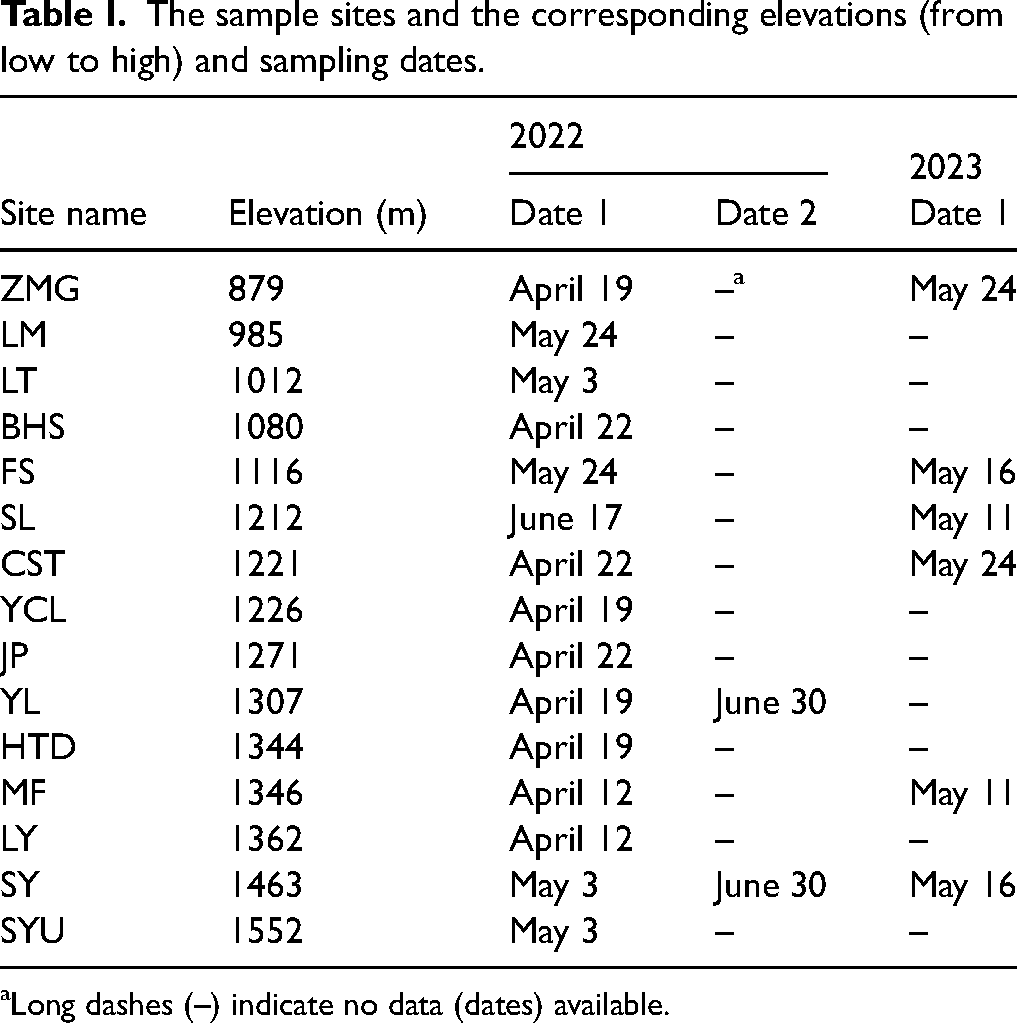
Long dashes (–) indicate no data (dates) available.

From each bag, we randomly selected 30 tea shoots to measure tea shoot spectra. Tea leaf reflectance and transmittance were assessed using a portable spectroradiometer (FieldSpec 3, Analytical Spectral Devices, Inc.) with a single integrating sphere (ASD RTS-3ZC). The spectral resolutions were 3 nm (between 350 and 1000 nm) and 10 nm (1000–2500 nm), with sampling intervals set at 1.4 and 2 nm, respectively. Due to the sizes of the sample ports of the integrating sphere (diameters ≥13 mm), we only measured the spectra of the third leaf (the largest one) for each tea shoot with one single-point measurement. To ensure the accuracy and reliability of the fresh tea leaf samples for subsequent biochemical analysis, each spectral reading was an average of 10 measurements. To assess the reflectance (Rs) and transmittance (Ts) of tea leaves, a non-polarized measurement method was employed by referring to the manufacturer-recommended procedure and Hovi et al.³⁰

R_{s} = \frac{(I_{s}^{R} - I_{d}^{R}) R_{r}}{(I_{c}^{R} - I_{d}^{R})}

(1)

T_{s} = \frac{(I_{s}^{T} - I_{d}^{T}) R_{r}}{(I_{u}^{T} - I_{d}^{T})}

(2)

where I_s represents the spectroradiometer readings taken from the tea leaf sample, I_c indicates the calibrated white reference, I_u is the uncalibrated white reference, and I_d denotes the stray light measured using a light trap. Superscripts R and T denote reflectance and transmittance, respectively, and R_r indicates the reflectance factor of the calibrated white reference. The procedure effectively measures the directional reflectance and transmittance factors;^28,31 the terms “leaf reflectance” and “leaf transmittance” are used for simplicity.

One major issue with spectral data collection in a moist region such as Taiwan is that high humidity may introduce erroneous signals.^32–34 Hence, we employed a statistical/mathematical spectral reconstruction approach to retrieve noise-free fresh tea leaf spectra involving spectral database matching, multivariable linear regression, linear parameter multiplication, and spectral reversion (Figure 1). The spectral preprocessing and reconstruction were detailed in Denaro et al.³⁵ and here we only briefly describe the procedure. First, the spectral databases were preprocessed through several steps including outlier removal and applying a low-pass filter to ensure data quality. Next, the spectral database is matched and modeled by comparing and aligning the spectral signatures with previously developed databases to identify the wavelength components. This is followed by multivariable linear regression, which utilizes multiple spectral variables to create a regression model predicting the spectral region of interest. Linear parameter multiplication was then applied to adjust the spectral data according to specific parameters. Finally, spectral reversion was performed to reconstruct the spectral region of interest from the transformed wavelengths, ensuring that the resulting spectra closely match the scale of the spectral data. There were 1016 pairs (total n = 2032) of reflectance and transmittance data collected in this study.

Figure 1.

Preprocessing of tea leaf reflectance (a) before and (c) after the spectral reconstruction, and transmittance (b) before and (d) after the spectral reconstruction data. The solid and dashed yellow lines depict the mean ± SD of each spectral band value.

Tea Flavor-Related Chemical Compound (TFCC) Analysis

Leaf samples (n = 30) were returned to the polyethylene bags (total = 36 bags) after leaf spectral measurement, and the samples were then immediately placed in a −20 °C cold storage unit until TFCC analysis. We note that instead of using the spectrally measured leaf,²⁵ we processed an entire tea shoot (an apical bud and three leaves) since tea makers use the former one to manufacture dried tea products. The HPLC analysis was applied to confirm the content of each TFCC from the tea shoot samples. For HPLC analysis, each sample required a minimum of 15 shoots; therefore, each bag was divided into three replicates for analysis. These samples were freeze-dried, ground into a fine powder, and sifted through a 4 mm sieve. Then, 0.5 g of this homogeneous tea powder was immersed in 50 mL of boiling deionized water for 20 min in a water bath held at 90 °C. The obtained tea infusions were subsequently filtered via 0.45 μm syringe filters in preparation for HPLC analysis. The HPLC analysis was set up using a Shimadzu system (PU-2089, AS-2057, UV-2075 detector; Shimadzu) with an equipped C18 column (5 μm × 4.6 mm × 250 mm; Waters). Solvents A (0.1% formic acid aqueous solution) and B (acetonitrile) were introduced following a specific gradient, which involved a linear increment of Solvent B from 1% to 10% over 15 min, subsequently escalating from 10% to 20% in the next 14 min, then further increasing from 20% to 22% within 6 min, and lastly maintaining the 22% concentration for an additional 5 min. A flow rate of 1.0 mL/min was maintained throughout the separation process. Absorbance was monitored at 280 nm for real-time tracking of peak intensities. The TFCC components, GA, CAF, and eight catechin isomers (GC, EGC, C, EC, EGCG, GCG, ECG, and CG), were commercially sourced from Sigma-Aldrich. Each compound was individually prepared at appropriate concentration ranges using standard solutions and then uniformly combined into a standard cocktail.¹⁴ The mixture was analyzed using the same liquid chromatography method, and a regression analysis was conducted by correlating the predetermined concentrations of each compound with their corresponding peak areas in the HPLC chromatograms to establish calibration curves. These calibration curves were subsequently used to determine the concentration of each compound in the samples. All samples were analyzed in triplicate to ensure consistency and accuracy (n = 108).

Deep Learning (Y-Net)

Data Augmentation

To develop a robust deep-learning model for learning and optimization, it is essential to acquire sizable spectral and TFCC data sets. However, it is not feasible to produce a large number of samples of TFCCs for deep learning using HPLC due to the nature of the analytical procedure. To mitigate this technical challenge, a simplified approach was adopted using an augmentation process.^36–38 The rationale for employing the augmentation process stems from the typically distributed correlation between spectral and biochemical characteristics, similar to the principles applied in Gaussian processes.³⁹ Hence, the augmentation involves using a normal distribution and requires the mean and SD from each bag of TFCC samples to simulate 30 TFCC data to match the sample size of reflectance and transmittance data (illustrated in Figure 2a). This augmentation technique facilitates expanding the data set and increases the variation of the available data, thereby enhancing the training process and improving the ability of the model to generalize new data (cf. Chen et al.⁴⁰ and Wieland et al.⁴¹).

Figure 2.

The workflow of using Y-net to estimate TFCCs with tea shoot reflectance and transmittance. (a) Illustration of augmented (gray circles) from observed (black circles) data. (b) Y-Net-based ResNet structure for TFCC prediction. (c) Convolutional block of ResNet, Y-Net. (d) Two-stage training: top (the first stage) and bottom (the second stage).

Y-Net Structure

Y-Net is a specific architecture that utilizes feedforward neural networks (FNNs) or CNN-based ResNet approaches.^42,43 The algorithm can take both reflectance and spectrally corresponding transmittance as input (Figure 2b). The Y-Net architecture consists of a one-dimensional (1D) convolution block (Figure 2c), 1D max-pooling, fusion, and fully connected layers. The process can be categorized into three steps, including feature extraction, fusion extraction, and TFCC prediction:

Feature extraction: This step comprises the encoder, which consists of six processes responsible for extracting meaningful features from the input spectral data. The input dimension was ∼2101 × 1, indicating one channel and a 1D spectral array with 2101 data points. The symbol ∼ represents the number of sample data corresponding to 36 data sets here. The processes numbered 1, 3, and 5 involved convolutional blocks which were part of the ResNet processing design, and those with 2, 4, and 6 entailed max-pooling operations (Figure 2c). The convolutional block operation used six layers including convolution, batch normalization, activation, and residual layer added to the last layer (Figure 2d). The kernel size was 1 × 5, indicating that the convolution operation was performed in the spectral windows with a stride of one and using padding to preserve the data dimension. Each convolutional block comprised several kernel filters, and an increased number of kernel filters in each block reduced the spectral dimension. This convolutional block was responsible for feature extraction, mitigating the vanishing gradient problem and preserving information across layers. The max-pooling process occurred between convolutional blocks and was applied to a 1D array using a window size of two. It found the maximum value within each window and applied a stride of two, meaning it moved by two positions at a time. A rectified linear unit function was employed as the activation function in this architecture. It introduced nonlinearity by setting negative values to zero and leaving positive values unchanged. The feature extraction step had six convolutional blocks (three reflectance and three transmittance branches). Each corresponding convolutional block (reflectance and transmittance) had a various number of parameters, e.g., [6, 4, 6, 4, 6], [12, 8, 22, 8, 12], and [44, 16, 84, 16, 44], in which the total parameters are 584, and these parameters corresponded to the weights, normalization, and biases in the filter masks; where each convolutional block stood for [conv, norm, conv, norm, conv]. These parameters were responsible for capturing and learning the patterns within the data.

Fusion extraction: The fusion extraction consisted of three processes numbered 7, 8, and 9 (Figure 2c). The fusion process combined the outputs of the right (reflectance) and left (transmittance) processes. It merged the information from these two sources using convolutional block and max-pooling operation, resulting in a fused single processing operation. In the fusion extraction step, one convolutional block fused the reflectance and transmittance branches. It consisted of five parameters, which were [conv, norm, conv, norm, conv], respectively. The total number of unknown parameters in the fusion extraction step was 1048. These parameters included normalization, weights, and biases associated with the convolutional and max-pooling operations.

TFCC prediction: The process involved in transitioning from the convolutional to the dense processes. This transition included flattening and dropping the data, which converted it from a 2D representation (0-axis for spectral and 1-axis for kernel filters) to 1D dense vectors and passed it through fully connected layers. The reshaped vector had a length of 2090 (Figure 2b, step 10), which was determined by the size of the output from the last max-pooling in the previous step, which has the dimension ∼26 × 128. The vector was then connected to a hidden layer with 10 neurons (Figure 2c, step 11), representing the 10 TFCC components of the first data set. In the TFCC estimation step, there were 2090 unknown parameters with weights and biases.

A total of 3722 parameters were utilized for optimizing Y-Net, encompassing both the convolutional block and fully connected layers. Studies employed FNNs to determine the optimal neural network structure and parameters, such as filter sizes, number of filters, layers, neurons, and activation functions.^44,45 However, this process often involves trial and error and can be time-consuming. Moreover, due to limited experimental data samples and the potential for overfitting, finding the optimal neural structure with the best parameters may not always be feasible. Therefore, this study adopted an alternative strategy by emphasizing the design of the steps within the neural structures rather than exclusively pursuing the optimization of parameters.

Y-Net Transfer Learning

The training of Y-Net was performed in two stages. In the first stage of training, we applied data augmentation to 1016 samples from 36 batches. In the second stage, we conducted bootstrapping (with replacement) of the data from 36 batches into training (70% of the data) and testing (30%) sets. The number of the observed points was less than the augmented points to train Y-Net.

During Y-Net training, observed data were less than the augmented ones. Hence, there were fewer actual data points available for training Y-Net. Utilizing the augmented data points made it possible to train Y-Net effectively despite the limited number of observed data points. In the initial stage of the two-stage training process (Figure 2d), the focus was on reaching a local optimum by adjusting the weights, biases, and dense parameters from their initial values. The second stage was designed to achieve the global optimum while also reducing the overall training time required to reach the optimal model. In other words, the initial parameters used in the second stage were derived from the pretrained model obtained during the first stage of training. This two-stage training approach optimized the model by first augmented data to reach a local optimum. Subsequently, it refined the model by experimental data to achieve the global optimum.

In the optimization process, we applied the built-in function RMSprop optimizer. It incorporates adaptive learning rate and moment techniques during training to reach the optimal model. We utilized the mean square error (MSE) as the loss function:

L = \frac{1}{n} \sum_{i = 1}^{n} (p r e d i c t e d_{i} - o b s e r v e d_{i})^{2}

(3)

where the

p r e d i c t e d_{i} = {\hat{c c}}_{j = 1}^{J}

and

o b s e r v e d_{i} = {c c}_{j = 1}^{J}

; j is the index of TFCC J, n is the number of data, and

c c

and

\hat{c c}

are observed and predicted TFCC, respectively. During the training process, a significant number of epochs were executed, and the number of epochs was set to 100. Throughout the training, the parameters of the epoch with the minimal loss value were stored. These optimal parameter values and the network structure were implemented to estimate TFCC.

Performance Assessment

To assess the effectiveness and viability of Y-Net, we conducted a comparative analysis by contrasting the performance of the two-stage training with that of the conventional one-stage training. We employed the two-stage training approach to determine whether the additional training stage would enhance model performance by referring to metrics losses. Furthermore, we also selected an advanced multivariate statistical (PLS) approach^46,47 and other commonly used machine-/deep-learning methods, including Cubist⁴⁸ with de-trend preprocessing,¹⁰ FNNs,^49–51 Gaussian processes,⁵² and RFs.⁵³ Since these methods have been commonly used in scientific literature, we only provide key references here for expedience. To assess the performances of these methods and Y-Net, we use the RMSE as the evaluation metric, as it measures the average deviation between the predicted and actual observed values. To further evaluate the consistency and stability of the models, we also took the mean and SD into account. Finally, we performed F-, T-, and Kolmogorov–Smirnov (K-S, non-parametric) tests to investigate statistical difference (equality) and distribution similarity of TFCC RMSE between Y-Net and other methods.

Y-Net Spectral Analysis

It is important to understand the contribution of different tea shoot spectral regions to estimate TFCC in Y-Net. Therefore, we carried out a spectral feature importance analysis. The feature important analysis took the features of each hidden layer in reflectance and transmittance branches. From the first layer of each branch to the fusion layers, we resampled, averaged, and normalized those to the scale of 0–1 to assess their importance to TFCC prediction. The feature importance analysis can be categorized into the local and global aspects to identify the pattern. The global pattern constitutes a significant contribution that can be visually identified, whereas the local pattern represents a minor contribution that requires a tool to unveil subtle information. Therefore, the high-pass filter was also adopted using a fast Fourier transform to enhance the minor contribution by capturing the high frequency in the feature importance.⁵⁴ In addition, we carried out a spectral subset analysis. We investigated if visible–near-infrared (Vis-NIR) spectral regions (400–1100 nm) would be sufficient to estimate TFCCs using Y-Net since they are responsive to photosynthesis/non-photosynthesis pigments (mainly chlorophyll a and b, carotenoids, xanthophylls, and anthocyanins)⁵⁵ and cell structure (e.g., the mesophyll cells and the fraction of air space)^56,57 of fresh green leaves. Therefore, Vis-NIR could be much more sensitive than leaf water content dominant shortwave infrared bands (∼1300–2500 nm).⁵⁸ Moreover, the spectroscopic measurement may be preferable within Vis-NIR due to the relatively higher energy throughput by referring to Planck's radiation law and more cost-effective for the instruments (silicon/InGaAs for Vis-NIR vs. InSb). Finally, we used tea shoot reflectance of the entire optical region only (without transmittance) for Y-Net since the physical property may be measured by airborne or spaceborne sensors permitting regional mapping of TFCC.

Results and Discussion

Input Data Assessment

To evaluate the performance of Y-Net, it is important to compare the data distribution of the observed data and augmented data (Figure 3). We found that they have similar characteristics by referring to statistics indicating the central tendency and spread of the data (Table SI, Supplemental Material). Therefore, the observed and augmented data have similar distributions, which justifies using the latter for further analysis. In addition, to investigate the data distribution of observed and augmented data, a loss value (MSE) comparison for 100 epochs was conducted in the optimization process (Figure 4). The optimization process provided two stages of training, with the first stage using augmented data and the second stage using observed data. There was an apparent improvement in the second stage, especially at the initial epoch; the difference in MSE became relatively negligible after 30 epochs. The performance of the two-stage training through this optimization was satisfactory by comparing the observed and predicted training and validation data (Figure 5 and Table SII, Supplemental Material). Overall, the data distributions of those groups were comparable except for some outliers of C, ECG, and CAF.

Figure 3.

(a) Observed (n = 114) and (b) augmented (n = 1135) TFCC including GA, CAF, and eight catechin isomers including GC, EGC, C, EC, EGCG, GCG, ECG, and CG.

Figure 4.

Epoch comparison for first and second stage learning. Mean squared error (MSE).

Figure 5.

Estimation of TFCC using Y-Net with tea shoot spectra: (a) observed training, (b) validation, (c) predicted training, and (d) validation data sets.

Model Performance Comparison

Y-Net underwent pretraining and acquired knowledge through a novel two-stage training approach (Figure 4), utilizing TFCCs from observed and augmented data (Figure 3 and Table SI, Supplemental Material). Overall, the performance of Y-Net (mean ± SD of RMSE = 0.65 ± 0.58) to model the variation of TFCCs was superior to (yielding the lowest mean and SD) selected statistical PLS (5.30 ± 5.02) and machine learning, including cubist (2.33 ± 2.18 mg g^–1), FNNs (2.39 ± 2.24 mg g^–1), Gaussian (8.44 ± 8.39 mg g^–1), and RF (2.49 ± 2.36 mg g^–1) (Table II; see also Table SIII, Supplemental Material, for parametric equality and non-parametric distribution similarity tests). The TFCC assessment of Y-Net was relatively consistent by referring to SD demonstrating its effectiveness across various compounds. However, the performance for modeling each TFCC differed.

Table II.

Performance comparison of selected statistics: PLS and machine-/deep-learning methods (cubist, three FNNs: FNN-1, FNN-2, and FNN-3), Gaussian process, RF, and Y-Net-based CNN) to estimate TFCCs using RMSE.

TFCC	PLS	Cubist	FNN-1	FNN-2	FNN-3	Gaussian	RF	Y-Net
GC	6.00	4.33	4.01	4.04	4.01	6.19	4.14	0.82^a
ECG	11.45	3.69	4.13	4.10	4.12	21.84	4.08	1.49
C	1.76	0.99	0.94	0.88	0.88	2.79	0.85	0.26
EC	2.84	1.24	1.24	1.24	1.20	3.88	1.27	0.35
EGCG	15.60	7.03	7.07	6.93	6.87	21.58	7.37	1.60
GCG	1.69	0.67	0.62	0.62	0.66	1.81	0.45	0.10
ECG	1.21	1.13	0.99	0.99	1.07	1.23	1.30	0.29
CG	0.02	0.04	0.13	0.16	0.07	2.83	0.05	0.04
GA	2.35	0.23	0.31	0.58	0.45	2.40	0.35	0.18
CAF	10.05	3.95	4.50	4.10	4.05	19.88	5.04	1.36
Mean	5.30	2.33	2.39	2.36	2.34	8.44	2.49	0.65
SD	5.02	2.18	2.24	2.15	2.14	8.39	2.36	0.58

The numbers in bold indicate the lowest values for each TFCC and the mean and SD.

Y-Net Spectral Analysis

According to our spectral feature importance analysis, several spectral regions of reflectance and transmittance were pivotal for modeling TFCCs; reflectance (55% of the optical spectral bands) played a more critical role than transmittance (45%) by referring to feature importance values (Figure 6). Specifically, after applying the high-pass filter (adopted with fast Fourier transform), spectral bands of reflectance and transmittance located around 400, 700, 1400, 1900, and 2500 nm were identified to be crucial for indirectly estimating TFCCs. The spectral subset analysis depicts that, overall, the Y-Net using both reflectance and transmittance of the entire optical region (400–2500 nm) (mean ± SD of RMSE = 0.65 ± 0.58 for training and 1.54 ± 1.5 for validation data sets, Table III) performed slightly better and relatively more consistent (with the lowest mean and SD) than the Vis-NIR (2.12 ± 2.15 and 3.15 ± 3.35) and the reflectance-only (1.71 ± 1.81 and 2.23 ± 2.25) Y-Nets. However, the performance of estimating each TFCC was different.

Figure 6.

Feature importance values of tea shoot optical spectra. Reflectance (ref.) and transmittance (trans.) in Y-Net. The high-pass (HP) filters can assess the local importance of the features; the higher values indicate that the local pattern can be affected significantly and vice versa.

Table III.

Y-Net performance comparison (RMSE) using spectra (reflectance and transmittance) from the whole optical (400–2500 nm) and Vis-NIR (400–1100 nm) regions and reflectance of the optical region only to estimate TFCC.

TFCC	Optical region		Vis-NIR		Reflectance
TFCC	Training	Validation	Training	Validation	Training	Validation
GC	0.82^a	2.79	2.86	3.55	1.84	3.90
ECG	1.49	2.69	4.14	8.56	3.50	4.20
C	0.26	0.42	0.71	0.93	0.47	0.54
EC	0.35	0.84	0.98	1.47	0.65	0.70
EGCG	1.60	4.75	7.14	10.26	5.99	7.18
GCG	0.10	0.14	0.41	0.34	0.30	0.43
ECG	0.29	0.94	1.03	1.45	0.94	1.25
CG	0.04	0.04	0.07	0.12	0.04	0.04
GA	0.18	0.15	0.41	1.06	0.43	0.41
CAF	1.36	2.60	3.43	3.79	2.99	3.61
Mean	0.65	1.54	2.12	3.15	1.71	2.23
SD	0.58	1.50	2.15	3.35	1.81	2.25

The numbers in bold indicate the lowest values for each TFCC, mean, and SD, separated by training and validation.

Y-Net Performance

The Y-Net architecture features a dual-branch input, integrating a ResNet-based CNN.^59,60 The dual input of Y-Net involves data augmentation or enrichment and pretraining through a novel two-stage training approach (Figures 2a and 2d), including utilizing TFCCs obtained from both augmented and observed data measurements. This unique process markedly improves the performance in predicting TFCCs, as evidenced by the initial epoch of the second-stage training involving pretraining using augmented data. Similar approaches have been found effective in deep learning tasks, where data augmentation significantly enhances model performance.³⁷ In particular, the dual-branch structure of Y-Net has shown promise in applications such as segmentation and feature extraction, further proving the potential of deep learning models with enriched data inputs.^38,43 The robustness of the method is also reflected in other domains, such as large-scale image-based applications, where learning domain-robust features led to the development of effective feature representations, further confirming its versatility and accuracy.²⁸ Compared to conventional machine-learning methods, the enhancement in performance is demonstrated (see Table II). The reduction in loss during this phase can be attributed to the utilization of pretrained parameters from the first-stage training in the second stage. This process serves a dual purpose: Preventing overfitting arising from limited observational data and augmenting the capacity for model generalization. Furthermore, this approach reinforces the adaptability and robustness of the model. It facilitates effective generalization of model performance across diverse data sets, utilizing data augmentation and chemical compounds (TFCCs) through feature extraction, fusion, and estimation (Figure 2b). Therefore, Y-Net becomes adept at capturing intricate data patterns with a specific focus on optimizing both local and global aspects during training. The local aspect of Y-Net involves capturing details or specific patterns of the input data. In contrast, the global aspect recognizes the overarching trend or general pattern spanning the entire data set. Additionally, integrating ResNet into the architecture addresses challenges such as vanishing gradients and ensuring information preservation across layers (Figures 2c and 2d). In summary, Y-Net outperforms other selected methods (PLS, cubist, FNN, Gaussian, and RF) for all TFCCs except CG by PLS and consistently achieves higher overall accuracy (Table II and Table SIII, Supplemental Material), making it a more reliable and comprehensive choice for TFCC estimation.

Spectral Importance to TFCC Retrieval Using Y-Net

To assess the performance of Y-Net, we aim to compare the spectral effectiveness of the optical region (400–2500 nm) using feature importance values by calculating the average feature extraction values in each branch, namely reflectance and transmittance. The average importance was derived from each convolutional block in the deep CNN (total of 37 layers). Each layer can yield results for feature importance, referred to as spectral contribution to predict TFCCs. In the hidden layers, higher spectral feature values contribute significantly to the prediction of TFCCs, whereas lower values indicate a comparatively less influential role in the predictive process. The analysis of spectral contributions across layers aids in understanding the significance of various features and their impact on accurately estimating TFCC concentrations by Y-Net throughout the optical range, particularly at 400, 700, 1400, 1900, and 2500 nm (Figure 6). To qualitatively identify patterns, encompassing both local and global aspects, and to isolate local patterns within the branch layers of reflectance and transmittance, a high-pass filter was employed in this study.^61,62 The high-pass filter adopts a fast Fourier transform that can enhance the minor contribution or local aspect by capturing the high frequency in the feature importance.⁵³ It is acknowledged that global aspects include visually apparent patterns such as trends and curves of the feature importance. Those global patterns are a significant contribution to TFCC prediction. On the other hand, interpreting local aspects may be challenging due to their minor contribution despite utilizing a substantial influence on TFCC prediction within specific wavelength regions. Using the high-pass filter, we can extract local patterns instead of considering them as interference, especially the feature importance in the deep layer networks. The local pattern was exhibited and appeared in the wavelength at around 400, 500, 700, 1150, 1400, 1900, and 2500 mm (Figure 6). These significant patterns are evident at the two ends of the optical region (400 and 2500 nm) and at 1900 nm, while lower significances were observed around 1150 and 1400 nm. The significant difference between reflectance and transmittance can be observed in their respective feature importance values across different wavelengths (Figure 6). The reflectance generally has higher feature importance values compared to transmittance, indicating that it plays a more critical role in the Y-Net model for predicting TFCCs. This difference suggests that the reflectance data contain more relevant information for the model to accurately predict the chemical compounds in tea shoots. The high-pass-filtered lines provide additional insights by highlighting the minor contributions and local patterns that might be otherwise overlooked in the original reflectance and transmittance data.

We also compared the spectral effectiveness of the optical region (reflectance and transmittance) with the models ingesting the Vis-NIR range of 400–1100 nm of reflectance and transmittance (due to a high signal-to-noise ratio and a cost-effective instrument), and reflectance only (for airborne and spaceborne remote sensing applications) of the entire optical region (Table III). Since the spectral patterns of green vegetation reflectance and transmittance are similar³⁸ (Figure 1), they yielded almost identical feature importance values (Figure 6). Thus, the reflectance method was adopted as the comparison in this study. The comparison was visually addressed using the feature importance and their high-pass filter, specifically for reflectance and transmittance, in each branch, while the transmittance was not used in the reflectance method. This implies that by employing Vis-NIR in the experiment, we neglect the significant important features and the less significant features in the spectral range of 1101–2500 nm (Table III, Vis-NIR), namely that evident in the spectral edges (400 and 2500 nm) and at 1900 nm. Therefore, the proposed Y-Net using entire optical region reflectance/transmittance outperformed the other two Y-Nets models. This is because, although they share almost identical important features and local patterns, they complement each other, with specific patterns present in spectral reflectance that may not be found in spectral transmittance. We also note that the performance of the Y-Net was merely slightly better than the Vis-NIR and reflectance-only Y-Nets. The spectral analysis demonstrates that we could reproduce similar outcomes with Y-Net using low-cost instruments. In addition, this study also underscores the potential of using airborne or spaceborne hyperspectral remote sensing for regional monitoring of TFCCs.

Y-Net Transfer Learning

Transfer learning is a deep learning technique where a model developed for a specific task is used as a starting point for training on a different task. It involves transferring parameters that capture general features, to enhance the learning process across various tasks. In the case of Y-Net, an advanced version of the FNN architectures, transfer learning is essential for improving its effectiveness on observation data tasks from the pretrained augmented data sets. Without transfer learning, predicting TFCCs with only observational data tends to have limited accuracy and generalization of the features, especially when dealing with small or complex data sets such as TFCCs. This often leads to false local maxima in the optimization process. Limited observational data can only train the model on a narrow range of chemical compounds, whereas a large data set provides a diverse spread of chemical information that Y-Net can learn for more general features. The availability of augmented data can help overcome these limitations by providing a broader feature space, allowing the model to learn more generalized patterns and improve its predictive performance. The augmented data cover a diverse range of chemical compounds, effectively supporting the learning tasks of the Y-Net model. This pretrained Y-Net model is then utilized as a basis for learning from the observational data sets.

Uncertainties and Limitations

While Y-Net demonstrates satisfactory performance (Table II), uncertainties exist, primarily attributed to the complexity of TFCCs. The intricate interactions and dependencies among various TFCCs pose challenges in achieving absolute precision. The performance of Y-Net is contingent on the quality and diversity of the training data, such as using additional augmented data (Figure 2a). Limited representation of specific chemical profiles in the training set may lead to challenges in accurately predicting less-represented compounds. For instance, the range of chemical compound values in augmented data may not be sufficient for effective Y-Net training. Expanding the range of compound values in Y-Net involves optimizing sensitivity and precision. Additionally, the generalization of Y-Net to diverse tea cultivars and physical environments could pose a limitation. The inherent variability in TFCCs across different varieties and growth environments could ramify the predictive accuracy. Continuous refinement and expansion of the training data set with actual data (without data augmentation) are crucial measures that could address some of these limitations over time. This ongoing effort aims to enhance the adaptability and robustness of Y-Net to a broader spectrum of TFCC profiles, ultimately improving its applicability across diverse environmental conditions and TFCCs. In addition, a potential limitation of Y-Net is its high computational power requirement. The complexity of processing and analyzing large volumes of data, especially when dealing with augmented data sets and diverse TFCC profiles, demands significant computational resources.

Conclusion

In this study, we proposed Y-Net, a deep-learning approach, to estimate TFCCs from fresh tea shoots indirectly using their optical reflectance and transmittance. We found that the performance of Y-Net was superior to some commonly employed advanced statistical (PLS) and machine-/deep-learning (cubist, FNNs, Gaussian, and RF) methods by referring to RMSE. The dual-input approach of Y-Net, considering both reflectance and transmittance simultaneously, outperformed those selected single-input models, providing a more comprehensive representation of TFCCs and improving predictive accuracy. Our spectral analyses showed that some specific bands located at 400, 500, 700, 1150, 1400, 1900, and 2500 nm were important for retrieving TFCCs. In addition, the reduction of the spectral range (Vis-NIR Y-Net) or exclusion of transmittance (reflectance only Y-Net) would also retard the overall performance. Taken together, these results emphasize the importance of advanced optimization techniques and the integration of multiple spectral data sources for precise chemical compound prediction in fresh tea shoots. Future research could focus on optimizing detection by enhancing the identification of key spectral bands and improving both the precision and efficiency of tea quality assessment. Furthermore, the advancement of spectral deep-learning techniques such as Y-Net holds significant potential for integration into field practices and quality control processes by enabling rapid and accurate chemical compound predictions, which can streamline decision-making and ensure consistent, high-quality tea production.

Supplemental Material

sj-docx-1-app-10.1177_27551857251338287 - Supplemental material for Spectroscopic Assessment of Flavor-Related Chemical Compounds in Fresh Tea Shoots Using Deep Learning

Supplemental material, sj-docx-1-app-10.1177_27551857251338287 for Spectroscopic Assessment of Flavor-Related Chemical Compounds in Fresh Tea Shoots Using Deep Learning by Lino Garda Denaro, Shu-Yen Lin and Cho-Ying Huang in Applied Spectroscopy Practica

Footnotes

Acknowledgments

We appreciate the field and lab assistance provided by Chi-Ching Huang, Yi-Ching Hung, and Zih-Yu Shen.

Data Availability Statement

All data used to support the findings of this study are available from the corresponding author upon request.

Declaration of Conflicting Interests

The authors declared no potential conflicts of interest with respect to the research, authorship, and/or publication of this article.

Funding

The authors disclosed receipt of the following financial support for the research, authorship, and/or publication of this article: This work was supported by the National Science and Technology Council (NSTC 112-2321-B-002-016), National Taiwan University (NTU-AS-112L104303), and the Research Center for Future Earth, the Featured Areas Research Center Program, the Higher Education Sprout Project, Ministry of Education (Taiwan).

ORCID iDs

Lino Garda Denaro

Shu-Yen Lin

Cho-Ying Huang

Supplemental Material

All supplemental material mentioned in the text is available in the online version of the journal.

References

Chen

Cai

Zheng

Yuan

, et al. “Quantitatively Unravelling the Impact of High Altitude on Oolong Tea Flavor from Camellia sinensis Grown on the Plateaus of Tibet”. Horticulturae. 2022. 8(6): 593. https://doi.org/10.3390/horticulturae8060539

Chen

Zhang

Huang

, et al. “Magnesium is a Nutritional Tool for the Yield and Quality of Oolong Tea (Camellia sinensis L.) and Reduces Reactive Nitrogen Loss”. Sci. Hortic. 2023. 308: 111590. https://doi.org/10.1016/j.scienta.2022.111590

Wang

Liu

, et al. “Characterization of Key Odorants in Lingtou Dancong Oolong Tea and Their Differences Induced by Environmental Conditions from Different Altitudes”. Metabolites. 2022. 12(11): 1063. https://doi.org/10.3390/metabo12111063

Ran

Zhang

, et al. “Comprehensive Analysis of Environmental Factors on the Quality of Tea (Camellia sinensis var. sinensis) Fresh Leaves”. Sci. Hortic. 2023. 319L: 112177. https://doi.org/10.1016/j.scienta.2023.112177

Dixon

R.A.

Strack

. “Phytochemistry Meets Genome Analysis, and Beyond”. Phytochemistry. 2003. 62(6): 815–816. https://doi.org/10.1016/s0031-9422(02)00712-4

Fang

Fernie

A.R.

Luo

. “Exploring the Diversity of Plant Metabolism”. Trends Plant Sci. 2019. 24(1): 83–98. https://doi.org/10.1016/j.tplants.2018.09.006

Rai

Saito

Yamazaki

. “Integrated Omics Analysis of Specialized Metabolism in Medicinal Plants”. Plant J. 2017. 90(4): 764–787. https://doi.org/10.1111/tpj.13485

Weng

J.K.

. “The Evolutionary Paths Towards Complexity: A Metabolic Perspective”. New Phytol. 2014. 201(4): 1141–1149. https://doi.org/10.1111/nph.12416

Yang

Kabahuma

Chaya

, et al. “A Gene Encoding Maize Caffeoyl-CoA O-Methyltransferase Confers Quantitative Resistance to Multiple Pathogens”. Nat. Genet. 2017. 49(9): 1364–1372. https://doi.org/10.1038/ng.3919

10.

Yamashita

Sonobe

Hirono

Morita

, et al. “Potential of Spectroscopic Analyses for Non-Destructive Estimation of Tea Quality-Related Metabolites in Fresh New Leaves”. Sci. Rep. 2021. 11(1): 4169. https://doi.org/10.1038/s41598-021-83847-0

11.

Hilal

Engelhardt

. “Characterisation of White Tea: Comparison to Green and Black Tea”. J. Verbraucherschutz Lebensmittelsicherh [J. Consum. Prot. Food. Saf.]. 2007. 2: 414–421. https://doi.org/10.1007/s00003-007-0250-3

12.

Pan

S.Y.

Nie

Tai

H.C.

Song

X.L.

, et al. “Tea and Tea Drinking: China’s Outstanding Contributions to the Mankind”. Chin. Med. 2022. 17(1): 27. https://doi.org/10.1186/s13020-022-00571-1

13.

Guo

Chen

Huang

, et al. “Optimization of Informative Spectral Variables for the Quantification of EGCG in Green Tea Using Fourier Transform Near-Infrared (FT-NIR) Spectroscopy and Multivariate Calibration”. Appl. Spectrosc. 2011. 65(9): 1062–1067. https://doi.org/10.1366/11-06287

14.

Lin

S.Y.

L.C.

Chen

I.Z.

Chen

P.A.

. “Effect of Shaking Process on Correlations Between Catechins and Volatiles in Oolong Tea”. J. Food Drug Anal. 2016. 24(3): 500–507. https://doi.org/10.1016/j.jfda.2016.01.011

15.

Ahmed

Griffin

T.S.

Kraner

Schaffner

M.K.

, et al. “Environmental Factors Variably Impact Tea Secondary Metabolites in the Context of Climate Change”. Front. Plant Sci. 2019. 10: 939. https://doi.org/10.3389/fpls.2019.00939

16.

Zhang

Cao

Q.Q.

Granato

Y.Q.

, et al. “Association Between Chemistry and Taste of Tea: A Review”. Trends Food Sci. Technol. 2020. 101: 139–149. https://doi.org/10.1016/j.tifs.2020.05.015

17.

Arumai Selvan

Mahendiran

Senthil Kumar

Kalilur Rahiman

. “Garlic, Green Tea, and Turmeric Extracts-Mediated Green Synthesis of Silver Nanoparticles: Phytochemical, Antioxidant, and In Vitro Cytotoxicity Studies”. J. Photochem. Photobiol. B. 2018. 180: 243–252. https://doi.org/10.1016/j.jphotobiol.2018.02.014

18.

Chen

Wang

C.Y.

Tsai

C.Y.

Yang

I.C.

, et al. “Fermentation Quality Evaluation of Tea by Estimating Total Catechins and Theanine Using Near-Infrared Spectroscopy”. Vib. Spectrosc. 2021. 115: 103278. https://doi.org/10.1016/j.vibspec.2021.103278

19.

Kang

Y.S.

Ryu

Suguri

Park

S.B.

, et al. “Estimating the Catechin Concentrations of New Shoots in Green Tea Fields Using Ground-Based Hyperspectral Imagery”. Food Chem. 2022. 370: 130987.

20.

Mao

Wang

Fan

, et al. “Prediction of Tea Polyphenols, Free Amino Acids, and Caffeine Content in Tea Leaves During Wilting and Fermentation Using Hyperspectral Imaging”. Foods. 2022. 11(16): 2537. https://doi.org/10.3390/foods11162537

21.

Huang

Wang

Jin

, et al. “Intelligent Evaluation of Storage Period of Green Tea Based on VNIR Hyperspectral Imaging Combined with Chemometric Analysis”. Infrared Phys. Technol. 2020. 110: 103450. https://doi.org/10.1016/j.infrared.2020.103450

22.

Merzlyak

M.N.

Melo

T.B.

Razi Naqvi

. “Estimation of Leaf Transmittance in the Near Infrared Region Through Reflectance Measurements”. J. Photochem. Photobiol. B. 2004. 74(2-3): 145–150. https://doi.org/10.1016/j.jphotobiol.2004.03.003

23.

Lee

M.S.

Hwang

Y.S.

Lee

Choung

M.G.

. “The Characterization of Caffeine and Nine Individual Catechins in the Leaves of Green Tea (Camellia sinensis L.) by Near-Infrared Reflectance Spectroscopy”. Food Chem. 2014. 158: 351–357. https://doi.org/10.1016/j.foodchem.2014.02.127

24.

Schulz

Engelhardt

U.H.

Wegent

Drews

H.H.

Lapczynski

. “Application of Near-infrared Reflectance Spectroscopy to the Simultaneous Prediction of Alkaloids and Phenolic Substances in Green Tea Leaves”. J. Agric. Food Chem. 1999. 47(12): 5064–5067. https://doi.org/10.1021/jf9813743

25.

Huang

Dong

Sanaeifar

Wang

, et al. “Development of Simple Identification Models for Four Main Catechins and Caffeine in Fresh Green Tea Leaf Based on Visible and Near-Infrared Spectroscopy”. Comput. Electron. Agric. 2020. 173: 105388. https://doi.org/10.1016/j.compag.2020.105388

26.

Wang

Y.J.

Jin

S.S.

M.H.

Liu

, et al. “Onsite Nutritional Diagnosis of Tea Plants Using Micro Near-Infrared Spectrometer Coupled with Chemometrics”. Comput. Electron. Agric. 2020. 175: 105538. https://doi.org/10.1016/j.compag.2020.105538

27.

Mehta

Mercan

Bartlett

Weaver

, et al. “Y-Net: Joint Segmentation and Classification for Diagnosis of Breast Biopsy Images”. Paper presented at: Medical Image Computing and Computer Assisted Intervention: MICCAI 2018. Granada, Spain; 16–20 September 2018. Pp. 893–901. https://doi.org/10.1007/978-3-030-00934-2_99

28.

Rao

Guo

, et al. “A Y-Net Deep Learning Method for Road Segmentation Using High-Resolution Visible Remote Sensing Images”. Remote Sens. Lett. 2019. 10(4): 381–390. https://doi.org/10.1080/2150704X.2018.1557791

29.

Tömösközi

Fitzek

F.H.P.

. “Y-Net: A Dual Path Model for High Accuracy Blind Source Separation”. IEEE Globecom (GC) Workshops. Taipei, Taiwan; 7–11 December 2020. 9367428. https://doi.org/10.1109/GCWkshps50303.2020.9367428

30.

Hovi

Forsström

Mõttus

Rautiainen

. “Evaluation of Accuracy and Practical Applicability of Methods for Measuring Leaf Reflectance and Transmittance Spectra”. Remote Sens. 2018. 10(1): 25. https://doi.org/10.3390/rs10010025

31.

Greiner

M.A.

Duncan

B.D.

Dierking

M.P.

. “Bidirectional Scattering Distribution Functions of Maple and Cottonwood Leaves”. Appl. Opt. 2007. 46(25): 6485–6494. https://doi.org/10.1364/ao.46.006485

32.

Simic

Chen

J.M.

Leblanc

S.G.

Dyk

, et al. “Testing the Top-Down Model Inversion Method of Estimating Leaf Reflectance Used to Retrieve Vegetation Biochemical Content Within Empirical Approaches”. IEEE J. Sel. Top. Appl. Earth Obs. Remote Sens. 2014. 7(1): 92–104. https://doi.org/10.1109/JSTARS.2013.2271583

33.

Noda

H.M.

Motohka

Murakami

Muraoka

, et al. “Reflectance and Transmittance Spectra of Leaves and Shoots of 22 Vascular Plant Species and Reflectance Spectra of Trunks and Branches of 12 Tree Species in Japan”. Ecol. Res. 2014. 29: 111. https://doi.org/10.1007/s11284-013-1096-z

34.

Irinislimane

Belhaneche-Bensemra

. “Application of Fourier Transform Infrared (FT-IR) Spectroscopy to the Study of the Modification of Epoxidized Sunflower Oil by Acrylation”. Appl. Spectrosc. 2012. 66(12): 1420–1425. https://doi.org/10.1366/12-06599

35.

Denaro

Chong

Huang

. “Reconstructing Fresh Green Leaf Spectra in the SWIR-2 Region (2001–2500 nm) Collected in a Humid Environment by Referring to Publicly Available Green Leaf Spectral Databases”. Int. J. Appl. Earth Obs. Geoinf. 2024. 129: 103842. https://doi.org/10.1016/j.jag.2024.103842

36.

Lashgari

Liang

Maoz

. “Data Augmentation for Deep-Learning-Based Electroencephalography”. J. Neurosci. Methods. 2020. 346: 108885. https://doi.org/10.1016/j.jneumeth.2020.108885

37.

Zhou

Dong

Liu

, et al. “Forecasting Emerging Technologies Using Data Augmentation and Deep Learning”. Scientometrics. 2020. 123: 1–29. https://doi.org/10.1007/s11192-020-03351-6

38.

Kargar

Zorbas

Gaffney

O’Flynn

, et al. “Y-Net: Insect Counting and Segmentation Using Deep Learning on Embedded Devices”. 2024 IEEE International Instrumentation and Measurement Technology Conference (I2MTC). Glasgow, UK; 20–23 May 2024. https://doi.org/10.1109/I2MTC60896.2024.10561007

39.

Van Wittenberghe

Verrelst

Rivera

J.P.

Alonso

, et al. “Gaussian Processes Retrieval of Leaf Parameters from a Multi-Species Reflectance, Absorbance, and Fluorescence Dataset”. J. Photochem. Photobiol. B. 2014. 134: 37–48. https://doi.org/10.1016/j.jphotobiol.2014.03.010

40.

Chen

Wei

Yao

Chen

, et al. “Data Augmentation in Prototypical Networks for Forest Tree Species Classification Using Airborne Hyperspectral Images”. IEEE Trans. Geosci. Remote Sens. 2022. 60: 1–16. https://doi.org/10.1109/TGRS.2022.3168054

41.

Wieland

Martinis

. “Multi-Sensor Cloud and Cloud Shadow Segmentation with a Convolutional Neural Network”. Remote Sens. Environ. 2019. 230: 111203. https://doi.org/10.1016/j.rse.2019.05.022

42.

Lan

Jiang

Yang

Gao

, et al. “Y-Net: Hybrid Deep Learning Image Reconstruction for Photoacoustic Tomography In Vivo”. Photoacoustics. 2020. 20: 100197. https://doi.org/10.1016/j.pacs.2020.100197

43.

Liu

Wang

Chen

Bian

, et al. “Y-Net: Learning Domain Robust Feature Representation for Ground Camera Image and Large-Scale Image-Based Point Cloud Registration”. Inf. Sci. 2021. 581: 655–677. https://doi.org/10.1016/j.ins.2021.10.022

44.

Ojha

V.K.

Abraham

Snášel

. “Metaheuristic Design of Feedforward Neural Networks: A Review of Two Decades of Research”. Eng. Appl. Artif. Intell. 2017. 60: 97–116. https://doi.org/10.1016/j.engappai.2017.01.013

45.

Paliwal

Kumar

U.A.

. “Assessing the Contribution of Variables in Feed Forward Neural Network”. Appl. Soft Comput. 2011. 11(4): 3690–3696. https://doi.org/10.1016/j.asoc.2011.01.040

46.

dos Santos

G.L.A.A.

Reis

A.S.

Besen

M.R.

Furlanetto

R.H.

, et al. “Spectral Method for Macro and Micronutrient Prediction in Soybean Leaves Using Interval Partial Least Squares Regression”. Eur. J. Agron. 2023. 143: 126717. https://doi.org/10.1016/j.eja.2022.126717

47.

Teixeira dos Santos

C.A.

Lopo

Páscoa

Lopes

J.A.

. “A Review on the Applications of Portable Near-Infrared Spectrometers in the Agro-Food Industry”. Appl. Spectrosc. 2013. 67(11): 1215–1233. https://doi.org/10.1366/13-07228

48.

Agyeman

P.C.

Kingsley

Kebonye

N.M.

Khosravi

, et al. “Prediction of the Concentration of Antimony in Agricultural Soil Using Data Fusion, Terrain Attributes Combined with Regression Kriging”. Environ. Pollut. 2023. 316(Part 1): 120697. https://doi.org/10.1016/j.envpol.2022.120697

49.

. “Classification of Black Tea Leaf Water Content Based on Hyperspectral Imaging”. 2023 IEEE International Conference on Control, Electronics, and Computer Technology (ICCECT). Jilin, China; 28–30 April 2023. https://doi.org/10.1109/ICCECT57938.2023.10140398

50.

Poggialini

Campanella

Legnaioli

Raneri

, et al. “Comparison of Convolutional and Conventional Artificial Neural Networks for Laser-Induced Breakdown Spectroscopy Quantitative Analysis”. Appl. Spectrosc. 2022. 76(8): 959–966. https://doi.org/10.1177/00037028221091300

51.

Wahl

Sjödahl

Ramser

. “Single-Step Preprocessing of Raman Spectra Using Convolutional Neural Networks”. Appl. Spectrosc. 2020. 74(4): 427–438. https://doi.org/10.1177/0003702819888949

52.

Holmes

W.S.

Ooi

M.P.-L.

Abeysekera

Kuang

Y.C.

, et al. “On Machine Learning Methods to Estimate Cannabidiolic Acid Content of Cannabis sativa L. from Near-Infrared Hyperspectral Imaging”. 2023 IEEE International Instrumentation and Measurement Technology Conference (I2MTC). Kuala Lumpur, Malaysia; 28–30 April 2023. https://doi.org/10.1109/I2MTC53148.2023.10175994

53.

Weng

Xiang

Jia

, et al. “Synchronously Predicting Tea Polyphenol and Epigallocatechin Gallate in Tea Leaves Using Fourier Transform–Near-Infrared Spectroscopy and Machine Learning”. Molecules. 2023. 28(14): 5379. https://doi.org/10.3390/molecules28145379

54.

Qiao

Huang

. “Spectral-Spatial-Frequency Transformer Network for Hyperspectral Image Classification”. 2023 IEEE Sensors Applications Symposium (SAS). Ottawa, Canada; 18–20 July 2023. https://doi.org/10.1109/SAS58821.2023.10254115

55.

Ustin

S.L.

Gamon

J.A.

. “Remote Sensing of Plant Functional Types”. New Phytol. 2010. 186(4): 795–816. https://doi.org/10.1111/j.1469-8137.2010.03284.x

56.

Jacquemoud

Ustin

. “Leaf Optical Properties in Different Wavelength Domains”. Cambridge, UK: Cambridge University Press, 2019. Vol. 1, Chap. 6, Pp. 216–238.

57.

Klancnik

Vogel-Mikus

Kelemen

Vavpetic

, et al. “Leaf Optical Properties are Affected by the Location and Type of Deposited Biominerals”. J. Photochem. Photobiol. B. 2014. 140: 276–285. https://doi.org/10.1016/j.jphotobiol.2014.08.010

58.

Huang

C.Y.

Anderegg

W.R.L.

Asner

G.P.

. “Remote Sensing of Forest Die-Off in the Anthropocene: From Plant Ecophysiology to Canopy Structure”. Remote Sens. Environ. 2019. 231: 111233. https://doi.org/10.1016/j.rse.2019.111233

59.

Andrew

Apan

Paudyal

D.R.

Perera

. “Convolutional Neural Network-Based Deep Learning Approach for Automatic Flood Mapping Using NovaSAR-1 and Sentinel-1 Data”. ISPRS Int. J. Geo-Inf. 2023. 12(5): 194. https://doi.org/10.3390/ijgi12050194

60.

Lee

C.P.

Lim

K.M.

Song

Y.X.

Alqahtani

. “Plant-CNN-ViT: Plant Classification with Ensemble of Convolutional Neural Networks and Vision Transformer”. Plants (Basel). 2023. 12(14): 2642. https://doi.org/10.3390/plants12142642

61.

Yoo

S.H.

Huang

Hong

K.S.

. “Physiological Noise Filtering in Functional Near-Infrared Spectroscopy Signals Using Wavelet Transform and Long-Short Term Memory Networks”. Bioengineering (Basel). 2023. 10(6): 685. https://doi.org/10.3390/bioengineering10060685

62.

Blaney

Fernandez

Sassaroli

Fantini

. “Dual-Slope Imaging of Cerebral Hemodynamics with Frequency-Domain Near-Infrared Spectroscopy”. Neurophotonics. 2023. 10(1): 013508. https://doi.org/10.1117/1.NPh.10.1.013508

Supplementary Material

Please find the following supplemental material available below.

For Open Access articles published under a Creative Commons License, all supplemental material carries the same license as the article it is associated with.

For non-Open Access articles published, all supplemental material carries a non-exclusive license, and permission requests for re-use of supplemental material or any part of supplemental material shall be sent directly to the copyright owner as specified in the copyright notice associated with the article.

0.00 MB

0.28 MB