Dispersed Images of the Partially Eclipsed Sun and Solar Corona as Proxies for Spectrometer Nonidealities

Abstract

Limitations in spectrograph behavior are difficult to visualize because aberrations, noise, and nonlinearity are largely mitigated in modern designs. Nevertheless, spectral resolution and precision are often subtly degraded by coma, astigmatism, stray light, noise, and distortion. The unique source geometry available during a solar eclipse allows a demonstration of some of these effects. Images from the eclipse of 8 April 2024 are presented and discussed.

Graphical abstract

This is a visual representation of the abstract.

Introduction

Real instruments make imperfect measurements of physical phenomena. Visualizing the imperfections is challenging not only because they may be subtle but also because the source of imperfection may be obscure, deeply buried in the hardware, or the result of multiple interacting components. For example, what is the shape of an atomic emission line? The shape depends on the atom's structure, electric and magnetic fields perturbing energy levels, thermal or optical excitation rate, excited state lifetime, and physical motion. Moreover, the observed line shape depends on instrument characteristics. Focusing on dispersive instruments, the shape is influenced by prism or grating dispersion, instrument aperture, number of dispersing elements, detector granularity, detector dynamic range and offset, various noise sources, stray light, and optical aberrations. Slit or entrance aperture width and focus may also matter. The range of factors influencing observation is vast.

A unique opportunity to exfoliate some of these factors is an observation of a solar eclipse. Prior to totality, sunlight is a reticulated continuum. Solar surface temperature approximates a 5800 K blackbody. Sunspots, flares, prominences, atomic absorption in the corona, and atmospheric atomic and molecular absorbance distort the blackbody curve, but at low resolution the approximation of solar radiation as a continuum is apt. During a total eclipse, however, only the corona is visible. The corona appears white to the naked eye and is composed of both continuum and line radiation. Provided a suitable filter is available to block intense sunlight outside of totality, a spectrograph can obtain images of both the sun and corona in close temporal proximity but with the shape of the emission source drastically different. Before totality, the sun is a shrinking crescent. In totality, it is a huge, circular source with a hole in the middle. Thus, concepts of the influence of source shape and optical distortion on spectra are readily seen.

Images reported here were recorded during the total solar eclipse of 8 April 2024. A smartphone camera, purpose-specific application program, and camera mounting hardware that allowed rapid parameter adjustment were used. Nothing that is reported here is fundamentally new; much of it was known by the middle of the 20th century. However, the data and explanations may prove useful in teaching optical and spectroscopic concepts.

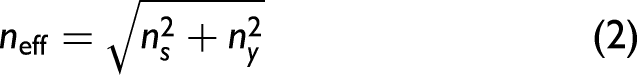
Spectra are generated using a double-axis transmission diffraction grating. The grating is a pattern embossed on Mylar resulting in a precise square pattern of raised stipples, spaced by a distance d of 5.0 µm. This results in diffraction orders with two order numbers, n_x and n_y. Zero order is in the center of each image with spectra defined by:

$$n_{\mathrm{eff}}\lambda =d\sin \beta$$

(1)

$$n_{\mathrm{eff}}=\sqrt{n_s^2+n_y^2}$$

(2)

The usual meanings of λ (wavelength, in the same units as d) and β (diffraction angle) apply. Approximating imaging as that of a pinhole camera, the radius r(λ) at which light reaches a detector pixel depends on the focal length f and is given by

$$r=f\tan \beta$$

(3)

The diffraction angle can thus be removed from the expressions by noting

$$n_{\mathrm{eff}}\lambda =d\sin \left({\tan }^{-1}{\displaystyle \frac{r}{f}}\right)={\displaystyle \frac{rd}{\sqrt{f^2-r^2}}}$$

(4)

As the detector is pixelated, convenient units for r and f are pixels, while for d units of nanometers are preferred.

Experimental

Materials and Methods

All data were collected using a Samsung S20 5G (SM-G986U) cellular telephone using SolarSnap software (https://www.eclipseglasses.com/collections/solar-snap-eclipse-app/products/solar-snap-the-eclipse-app). A filter included with the software package was used to protect the camera except during totality. Between the filter and the camera entrance lens, a double-axis diffraction grating (https://www.rainbowsymphony.com/products/diffraction-grating-rolls?variant = 29137920193) was interposed. Note that the vendor claims the grating has 13 500 lines per inch or 531 lines per mm. In fact, our characterization indicates that the gratings are 500 lines per millimeter in each direction. ¹ As shown in Figure 1, the filter and grating were held in place with Velcro; alignment was stabilized with masking tape that also reduced (though did not eliminate) stray light. The phone/filter/grating stack was clamped to a tripod that, in turn, stood on three concrete blocks so that the phone was at a comfortable height. Early in the eclipse, the software was used to set focus (94% of focus to infinity); thereafter, the focus was only checked after the start of totality and was found not to have shifted. Partway through the partial eclipse, the camera was tilted so that the narrowest section of the solar arc was approximately aligned with the grating y-axis and the narrower aspect of the camera's rectangular field of view (offset ∼5°). Exposure and magnification were varied throughout the eclipse. Metadata automatically recorded by the software tracked effective focal length, exposure, and moment of exposure with a resolution of 1 min. The camera was located at latitude 38°, 44 min, 39.7 s north, 88°, 4 min, and 49.5° west in Olney, Illinois. The altitude above mean sea level was 110.23 m. The only obstruction to clear viewing was a high cirrus cloud. Images were 3024×4032 pixels, 8 bits/color, or 24 bits/JPG pixel.

Figure 1.

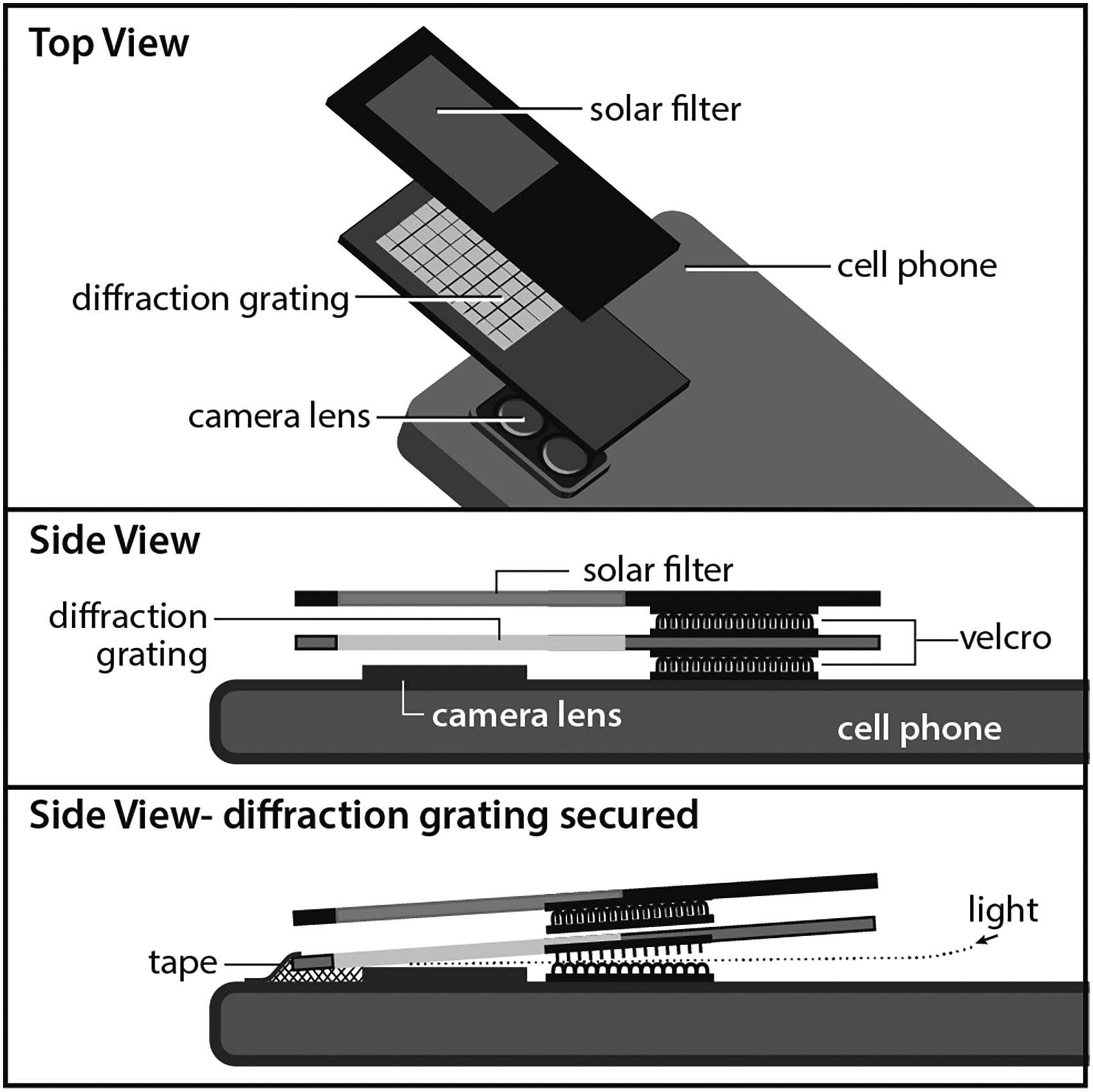
Grating and solar filter geometry. The double-axis diffraction grating was held by Velcro to the body of the cellphone, with the solar filter held by a second layer of Velcro above the grating until eclipse totality. To keep the x-axis of the grating parallel to the y-axis of the camera, the tape was employed (parallel to the long axis of the phone; the figure shows tape along the narrow axis for diagrammatic simplicity). Stray light can bypass the grating at an oblique angle, a problem prior to but not during totality.

Data were extracted using custom software coded in Embarcadero Delphi. The software was published through the Analytical Sciences Digital Library; ² the current hotlink is by Kelley and Scheeline. ³ Graphs were prepared in Excel and additional simulation software was coded in Delphi. Simulation software is included as Supplemental Material.

Results and Discussion

Data are based on three images, shown unprocessed in Figures 2–4. The first image is of the incompletely eclipsed sun approximately 2 min before totality. The other figures are of the totally eclipsed sun.

Figure 2.

Image of the partially eclipsed sun, 2:00 PM, approximately two minutes before totality. f/1.8, 1/16 s exposure, ISO-1059, focal length 5 mm, equivalent to a focal length of 26 mm for a 35 mm diagonal single lens reflex camera. The horizontal field of view is approximately ±30°. Vertical field of view approximately ±25°. Taken through a solar filter and diffraction grating.

Figure 3.

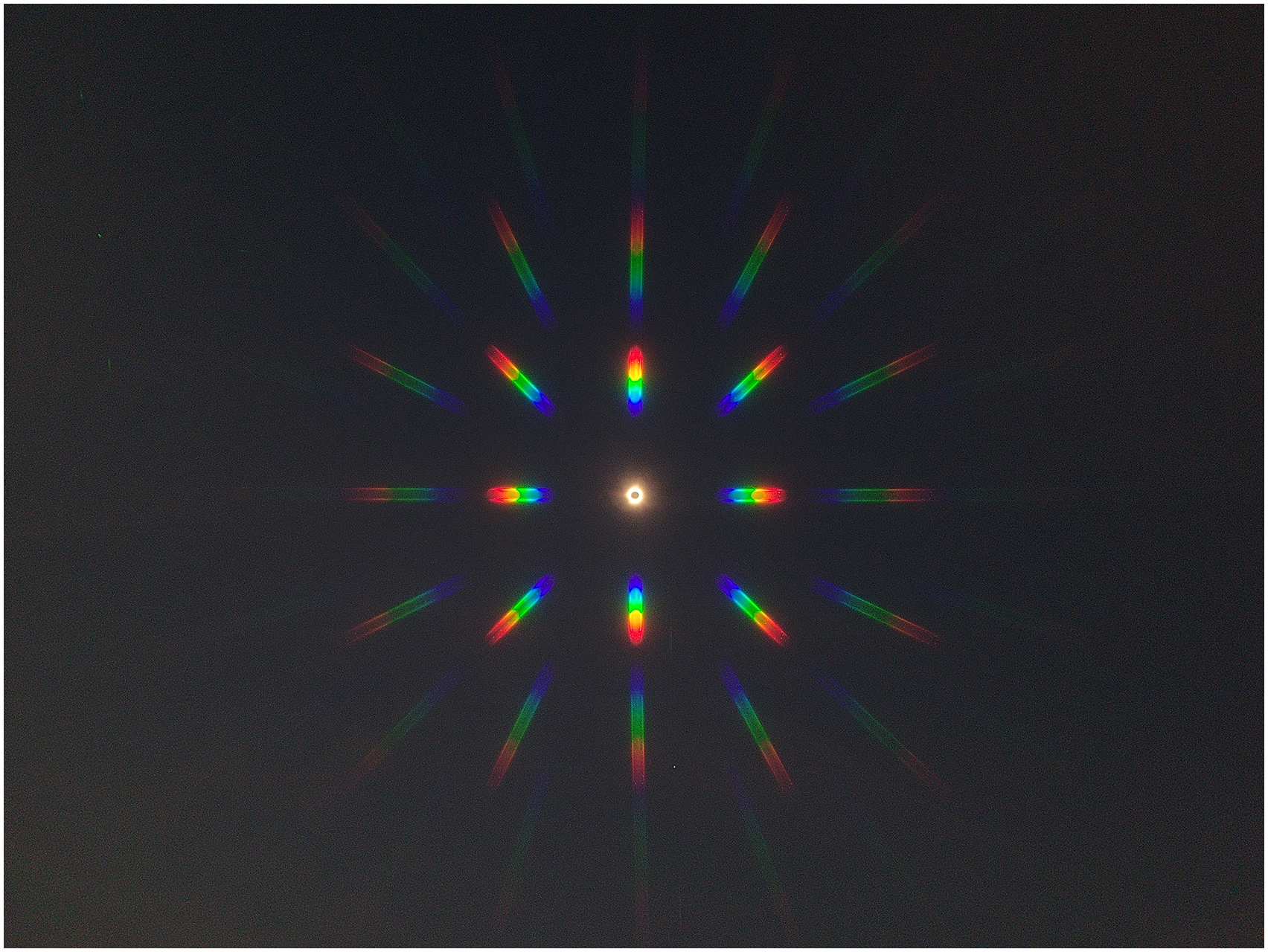
Image of totally eclipsed sun, 2:03 PM, approximately one minute after the start of totality. f/1.8, 1/33 s exposure, ISO-400, focal length 5 mm. Taken through diffraction grating only.

Figure 4.

Image of the totally eclipsed sun, 2:03 PM. f/1.8, 1/50 s exposure, ISO-360, focal length 5 mm but optically zoomed (zoom factor not recorded, but from the field of view, the zoom factor is approximately 2.4).

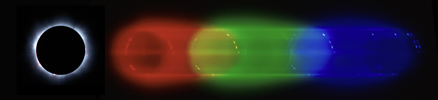
Double-axis gratings diffract identically along the x and y axes. If spectral appearance were due to diffraction alone, the horizontal and vertical spectra would be identical. They are not. Spectra along the y-axis (n_x= 0, n_y= ±1) are as wide as the solar crescent. Spectra along the x-axis (n_x= ±1, n_y= 0) are as high as the solar crescent but blurred along the dispersion direction as each point on the crescent acts as an independent light source. Spectral resolution is better along the y-direction than the x-direction. This would be easier to see if atomic lines rather than continua dominated the spectra, but the crescent's geometry allows easy visualization of the resolution difference. This is highlighted in Figure 5. The y-dispersed orders and crescent image from Figure 1 are copied to be adjacent to each other. For any given x-value, the y dispersion is the same (at least within the resolution of the pixels). The position of any wavelength, however, is with respect to zero order for the particular x-position within the crescent/light source. Thus, for n_y = +1, yellow bulges toward the red end of the spectrum, while for n_y= –1, yellow bulges toward the green end of the spectrum. Suppose one tries to improve signal levels or signal-to-noise ratio by averaging along a straight line parallel to the x-axis. For n_y = +1, wavelengths in the yellow (near 585 nm) will blur with longer (red) wavelengths, while for n_y= –1, yellow will blur with shorter (green) wavelengths. In spectrometers, this may be recognized in hardware, e.g., in Fastie–Ebert designs with curved entrance and exit slits. ⁴ In spectrometers with straight entrance slits, curved tangential focal images are inevitable, and integrating along the full slit height results in reduced resolution. The use of two-dimensional detection arrays may allow for image curvature compensation, but such compensation is wavelength-dependent since image curvature depends on the distance from the collimator/camera mirror vertex.^4,5

Figure 5.

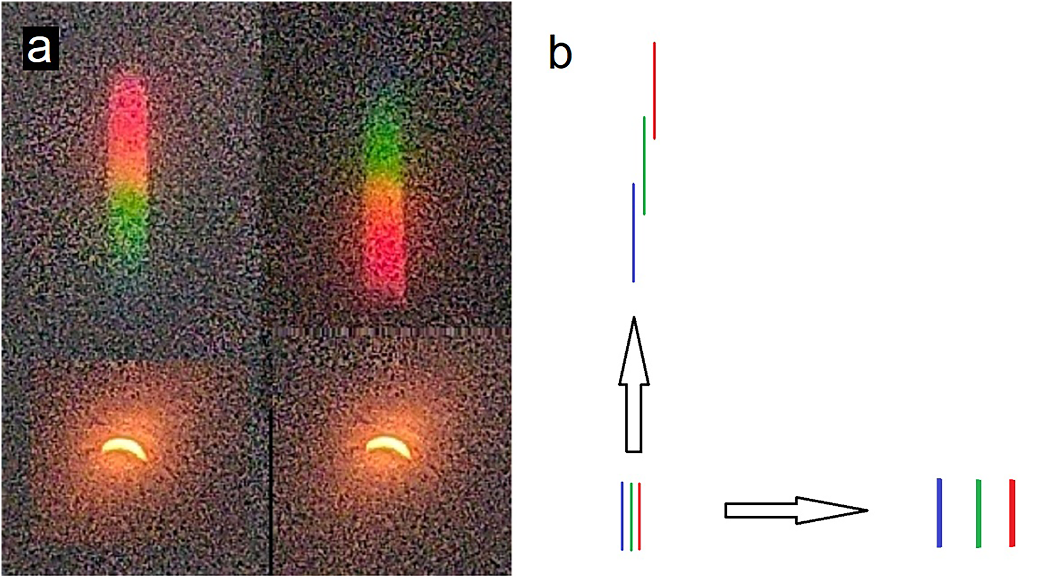
(a) Insets from Figure 2, show how dispersion is linear in the grating dispersion direction but curved to follow the shape of the observed object. The crescent serves the role of the entrance slit in an ordinary spectrograph. The yellow crescent is curved to follow the crescent sun, giving distortion towards the red for n_y = +1 (left side), and distortion towards the green for n_y= –1 (right side). The crescent sub-image is duplicated for ease of comparison. (b) In the limiting case of a narrow line source, dispersion in the x direction gives clean line separation, while in the y direction, the spatially extended sources result in spectral blurring.

Because of the graininess of the images, attempts to show quantitatively the qualitative features just described are not possible. To get a good signal-to-noise ratio, one must average over at least 11 pixels in y, which blurs data to a greater extent than the thickness of the crescent which is 8-pixels high. Averaging over three vertical pixels, with extraction aligned to be centered in x across the order and centered in the yellowest section of y, one obtains the data in Figure 6. It is tempting to suggest that the green level is the same for both n_y= 1 and n_y= –1, while red is higher (as expected) for n_y = +1 and blue is nearly entirely absent for n_y= –1. However, the noise is so great that one fears confirmation bias. Caveat lector.

Figure 6.

A plot of R, G, and B values in the yellow section of the dispersed insets in Figure 5.

Could the noise be non-random? The grating is mylar, 50 µm thick. With a refractive index of approximately 1.6, the optical thickness is thus 80 µm or 160 λ at 500 nm. However, light does not pass through the grating at normal incidence except at the center of the image. Thus, the grating also acts as a Fabry–Perot interferometer. For the optical depth to be 161 λ, light would need to traverse the grating substrate at an angle of tan^–1(1/160) or approximately 0.36°. In the small angle limit, for a perfectly flat substrate, modulation would thus occur in ∼1/3 degree increments across the field of view. The film is not optically flat, nor is its thickness controlled to submicron precision. The haze of noise is patterned on a scale smaller than the half-degree diameter of the sun/moon but approximately on the order of 5–10 pixels or ∼0.05°–0.1°. The graininess, then, is deterministic noise. A two-dimensional Fourier transform of the noise might reveal the departure from a constant thickness of the grating film.

Just as object curvature can degrade resolution, so coma, the variation of magnification across a focused image, decreases spectrum resolution. Even when coma is perfectly compensated at two wavelengths, there is some blurring elsewhere along a focal plane. ⁶ Whether such blurring is significant depends on the relative contributions of slit width, pixel width, and comatic aberration. Similarly, blurring here is a composite of the effects of noise, pixel size, and source size.

The top, and particularly the top right, of the image in Figure 2, is gray rather than black. Consistent with the geometry shown in Figure 1, this is stray light that finds its way to the camera by scattering off the cardboard mounts holding the grating and solar filter. Spacing between the camera/phone body, the grating, and the filter is inevitable as the mounting is Velcro, approximately 5 mm thick. During totality, low ambient light reduces the amount of stray light (Figures 3 and 4), but during partial eclipse light entering the gap between filter planes is inevitable. The edges of the grating could have been sealed against the phone body with opaque tape, but then the grating would have been less planar, further complicating interpretation of dispersion. Taping the solar filter in place would have prevented rapid removal at the beginning of totality, cutting the severely limited time available for data acquisition or for naked-eye observation of the corona and prominences.

Having exhausted analysis of the partial eclipse image, we now discuss images of the totally eclipsed sun. The solar filter was removed, a quick focus check confirmed that the optimum focus had not changed, the camera was zoomed out to allow photography of the corona and dispersed spectra, and then in rapid succession, various combinations of exposure and zoom were obtained. Figure 3 was selected as having the shortest exposure during totality that also had minimal stray light. In both Figures 2 and 3, saturation is seen to be greater for y-dispersed spectra than x-dispersed spectra. We can only speculate on why this is so. Because the only focusing occurs through the camera lens (i.e., light hitting the grating is not collimated), non-uniformities in the grating would result in wavelength-to-wavelength and order-to-order throughput differences, even absent vignetting. The lens entrance window is approximately 2 mm wide. In the y-direction, the third order is weakly visible; in the x-direction only orders up to two are visible. At 500 nm, the second order is at 11.5° while the third order is at 17.45°. For a field of view of ±20° and a gap from lens to grating of 2 mm (estimated, not measured), the lens observes through a pupil approximately 3.5 mm in diameter, encompassing 700 diffracting points along each axis and 500 $(700/\sqrt{2})$ along diagonals (or a total of 3.8 × 10⁵ diffracting spots). Interestingly, when data were extracted from this image, it was possible to pass the extraction line through the center of all x orders with n_y= 0, but a choice had to be made for y orders whether to center on dispersed orders or the zero-order corona image. The grating is out of plane (warped) vertically, and this appears to have influenced throughput as well as alignment (Figure S1, Supplemental Material).

Both Figures 3 and 4 show the dispersed corona spectrum has maxima aligned with the edge of the lunar disk/inner edge of the corona, with fall-off at greater offset from the spectrum centerline and also across the centerline. This illustrates structures commonly seen in laterally observed emission plasmas. Extracting red–green–blue (RGB) data from Figure 3 along the x-axis, through the center of the eclipsed sun, signal for each color is plotted in Figure 7a, with a scale-expanded view of the central image in Figure 7b. The encoded data have values from 0 to 255 for each color in each pixel. The extracted region is 5 pixels high, so the highest possible signal is 5 × 255 = 1275. While the exact camera model for the S20 phone camera is unavailable, Samsung does have a technology dubbed Isocell (https://semiconductor.samsung.com/image-sensor/) that provides a tricolor response in each pixel. Perhaps the fact that all three colors saturate or come close to saturating in the brightest part of the corona can be traced to such engineering. In any event, blue does not saturate.

Figure 7.

Summed intensities for Figure 3 along the central x-axis over a band 5-pixels high. (b) Expanded section of (b) showing only the undispersed corona cross-section. Note red and green pixels are saturated, but blue is not.

While all orders appear to align as described by Eqs. 1 through 4 and at an angle

$$\theta ={\tan }^{-1}{\displaystyle \frac{n_y}{n_s}}$$

(5)

careful examination of Figure 3 shows that there are small misalignments for orders with n_y ≠ 0. This too is shown in Figure S1 (Supplemental Material).

The corona subtends an angle of over 1°. The first order covers approximately 3.5°; the second order covers approximately 7°. Camera response spans approximately 400 to 700 nm. Thus, spectral resolution is too poor to see individual emission lines. Furthermore, the corona emits both line and continuum radiation. A higher spatial resolution example is available from the University of Montana online solar spectrum archive. ⁷ Helpfully annotated spectra are in section 2 of a related University of Montana web posting. ⁸ Based on the latter, a program, included in Supplemental Material, was written to mimic the observed data in the zoomed-in image of the eclipse (Figure 3). Simulated features include:

Spatial structure of the corona, assumed to be circular with a dark center, approximately 7 pixels of uniform bright emission, and then exponential falloff with a radial dependence of e^−0.025r with r in pixels from the edge of the bright emission ring. The outermost radius considered is 200 pixels (e^–0.025r at 200 pixels is e^–5; for a peak intensity of 255, the resulting intensity is two counts).

Line emission from Hα (656.3 nm), Hβ (486.1 nm), Hγ (434.0 nm), Hδ (410.2 nm), He I (584.3 nm), and additional lines weakly evident in the Montana REU spectra including Fe XIV (530.3 nm) and three other wavelengths (C I 447.8 nm, plus two unidentified lines near 518 nm).

Optionally, continuum. No attempt was made to estimate spectral variation of intensity, only spatial variation.

RGB camera response similar to that found for generic Bayer pattern cameras.

Figure 7b shows that approximating the central intensity as zero is inappropriate. Whether the signal is due to stray light, earthshine reflecting off the moon, blooming in the detector, or interpolation by camera firmware was not investigated. The results of the simulation are shown with (Figure 8a) and without (Figure 8b) including the continuum in the modeling.

Figure 8.

(a) Simulated dispersed spectrum including continuum. (b) Same, but without a continuum. Without continuum default relative intensity values as hard-coded in the software. With a continuum, intensity values have been adjusted for optimal appearance.

Conclusion

The poor spatial and spectral resolution evident in the eclipse images and spectra reported here is useful for visualizing nonidealities commonly present, though in more subtle form, in spectroscopic instruments. For much routine spectrometry, users ignore coma, nonlinearity, field curvature, and many other instrumental artifacts and simply report signal or relative signal at whatever wavelength appears when some routinely set wavelength is typed into control software or cranked into a manually scanned grating. Here we illustrated how spectra could be contaminated by easily anticipated or explained behavior (object curvature, grating departure from flatness, and signal saturation) and by other behavior not so readily understood (granular noise). If data are presumed to be adequate, instrument users may fail to seek out nonidealities similar to but more subtle than those illustrated here, to the detriment of experiment optimization and result validity.

Supplemental Material

sj-zip-1-app-10.1177_27551857241285464 - Supplemental material for Dispersed Images of the Partially Eclipsed Sun and Solar Corona as Proxies for Spectrometer Nonidealities

Supplemental material, sj-zip-1-app-10.1177_27551857241285464 for Dispersed Images of the Partially Eclipsed Sun and Solar Corona as Proxies for Spectrometer Nonidealities by Alexander Scheeline in Applied Spectroscopy Practica