
Abstract
Human activity is a key indicator of urban vitality. However, the spatially dependent and nonlinear relationships between urban landscape patterns and human activity intensity remains an underexplored area of research. Using the Luojia1-01 nighttime light data as a proxy for human activity intensity and fine-scale 3D building information to quantify urban landscape patterns, this study applied both the multiscale geographically weighted model (MGWR) and the extreme gradient boosting regression model (XGBoost) to investigating such relationships. Wuhan, the largest metropolis in Central China, was selected as the study area for the application of our methodology. The prediction results identified road area density and floor area ratio as the dominant factors affecting Nighttime light (NTL) intensity, while building height, building plan area ratio, and building volume ratio had minimal impacts. The same landscape metric in different built environments might have distinct impacts on NTL intensity, especially for the spatial dominance metrics like the 2D and 3D largest patch index. However, discrepancies were found between the two models, concerning the importance level and effect directionality of road length density and facade area ratio. This was due to the linear assumption adopted by MGWR, which might underestimate feature importance and obscure threshold effects when employing large bandwidths. Our findings highlighted significant impacts of urban landscape patterns on human activity intensity. The relationships tended to follow a simple nonlinear pattern, which were more effectively captured by the XGBoost model.
Keywords
Introduction
Over the past few decades, China has experienced rapid urbanization, which is primarily manifested in two aspects: urban expansion and densification (Broitman and Koomen, 2015; Cao et al., 2023). This transformative process has not only reshaped the physical landscape of cities but also exerted profound impacts across economic, social, and environmental domains (Gong et al., 2019). While rapid urbanization has generated substantial developmental space and economic opportunities, it has simultaneously revealed a critical misalignment between population and land urbanization rates (Shi et al., 2016; Sorace and Hurst, 2016). This misalignment reflects not only temporal disparities in development pace but also significant regional inequalities, manifesting in two distinct urban phenomena. On the one hand, major Chinese cities have witnessed the proliferation of urban villages, characterized by high population density and inadequate infrastructure, primarily due to rapid population influx and lagging urban development (Kochan, 2015; Zhao et al., 2021). On the other hand, newly developed urban areas, particularly in the peripheries of established urban cores, have experienced excessive spatial expansion disproportionate to actual demand, resulting in emergence of underutilized ‘ghost cities’ (Jin et al., 2017; Woodworth and Wallace, 2017). These urban development patterns present substantial challenges to sustainable urban growth, negatively impacting both economic efficiency and residents’ quality of life (Chen et al., 2015; Nugroho et al., 2022). Understanding the complex interplay between these spatial patterns and human dynamics is crucial for informing urban planning strategies and promoting sustainable urban development (Wiedmann and Allen, 2021).
Landscape metrics have been widely used to characterize the spatial patterns of cities. A growing body of research has shown that these metrics can effectively capture the physical characteristics of cities and their transformations from multiple perspectives, including size, shape, and composition. Traditional two-dimensional (2D) landscape metrics are adept at depicting urban expansion but face significant limitations when it comes to capturing urban densification, particularly in the vertical dimension. Fortunately, with the increasing availability of high-resolution satellite imagery and LiDAR data, an increasing number of studies has focused on three-dimensional (3D) landscape metrics to enhance the characterization of urban physical space (Berger et al., 2017; Kedron et al., 2019). Compared with the physical space of cities, the intensity and distribution of human activities are considerably more challenging to characterize. Although data such as points of interest (POI), public transportation, and mobile phone use can partially reflect the intensity of human activities, they often face challenges related to spatial coverage and temporal consistency (He et al., 2018; Jia and Ji, 2017; Sulis et al., 2018). Nighttime light (NTL) data offer an alternative option. A substantial body of literature has shown that NTL data can objectively capture the intensity and variation of urban human activities (Bennett and Smith, 2017; Chen et al., 2017). Particularly the advent of Luojia-1 satellite data, which provides higher spatial resolution information than the commonly used NTL datasets, has opened new possibilities for research at finer spatial scales (Cui et al., 2023; Ou et al., 2019). The material urban space itself does not possess vitality but has an impact on people’s behavior. As the carrier of human activity, urban physical space shapes how people interact and socialize while also defining the physical boundaries in which these activities occur (Frolking et al., 2013; Lanau et al., 2019). That is, the relationship between the two connects the social and material dimensions of urban life, clarifying how urban development interfaces with a multitude of socio-economic transformations (Wolff et al., 2020).
Studies have shown a significant correlation between urban landscape patterns and human activity intensity. Early studies often employed qualitative analyses or hierarchical quantitative frameworks to estimate human activity intensity. However, such approaches tended to oversimplify the spatial heterogeneity of human-environment interactions, and the reliance on subjective indicator weighting limited the generalizability of findings (Huang et al., 2020). Recently, the increasing availability of multisource data provides enhanced capabilities for objectively assessing human activity intensity. For example, Xu et al. (2022) adopted NTL as a proxy for human activity intensity and applied bivariate correlation analysis to examine the spatial relationship between building morphology and human activity intensity in Shanghai. The findings showed a similar spatial distribution pattern between the two, accompanied by an analysis of mismatch areas. However, the bivariate correlation cannot analyze the joint effects of multiple urban landscape indicators on human activity. Additionally, the assumption of the linear associations in this methodology may simplify the complex relationships between urban landscapes and human activities. Instead, machine learning models have garnered significant attention due to their ability to explore nonlinear relationships. For example, Wu et al. (2022) used extreme gradient boosting model to examine the relationships between urban landscape patterns and NTL intensity in Shanghai and Ningbo, China. This study revealed a complex nonlinear relationship between the two variables and demonstrated that the impact of 3D landscape metrics was greater than that of 2D metrics. Nevertheless, machine learning models inherently assume data independence during model fitting and thereby do not account for the spatial dependencies among variables. To date, research integrating spatial aware models with machine learning to investigate urban landscape-human activity interactions remains limited.
With the above issues in mind, this study is designed to investigate the relationships between urban landscape patterns and human activity intensity in the largest metropolis in Central China—Wuhan. Wuhan features a highly heterogenous urban landscape with thriving economy and dense population, providing an ideal backdrop for our research. In this study, we use fine-scale vectorized building data to map the urban landscape of Wuhan and employ high-resolution Luojia-1 NTL data as a proxy for human activity intensity. To investigate the relationships between urban landscape metrics and NTL intensity, we adopt a dual-model analytical framework. First, the multiscale geographically weighted regression model was applied to analyze the effects of multiple urban landscape metrics on NTL intensity with a consideration of spatial dependencies among the metrics. Meanwhile, the extreme gradient boosting machine learning model was employed to investigate these effects with a nonlinear assumption at a global scale. Our specific research objective was to answer the following questions: (1) What are the relationships between urban landscape patterns and NTL intensity in Wuhan? (2) How do the relationships vary spatially? (3) Are there discrepancies in the results generated by the two distinct modeling approaches and why?
Study area
Wuhan, the capital of Hubei province, is the largest city in Central China. It is located on the Jianghan Plain at the confluence of the Yangtze River and Han River, with a permanent population of 11.08 million and a gross domestic product of 1.48 trillion RMB in 2018 (NBSC, 2019). Wuhan has a subtropical monsoon climate with extremely hot and humid summer. As the national center of industry, education, and transportation, Wuhan has experienced rapid urbanization during the past decades. However, Wuhan is also a city rich in historical and cultural heritage with a solid industrial foundation, featuring a diverse urban landscape characterized by the coexistence of historical landmarks, aging buildings, factories, and modern architecture. Our study area focuses on the central urban area of Wuhan enclosed by the third ring road, covering approximately 655.6 km² and encompassing the Hanyang, Qiaokou, Jianghan, Jiang’an, Wuchang, Qingshan, and portions of the Hongshan districts (Figure 1). Qingshan and Qiaokou are recognized for their chemical and heavy industrial sectors. Jianghan, as the central urban district of Wuhan, serves as a key commercial hub. In comparison, Wuchang and Hongshan are more oriented towards culture and education, while also being the two most populous districts in the city.
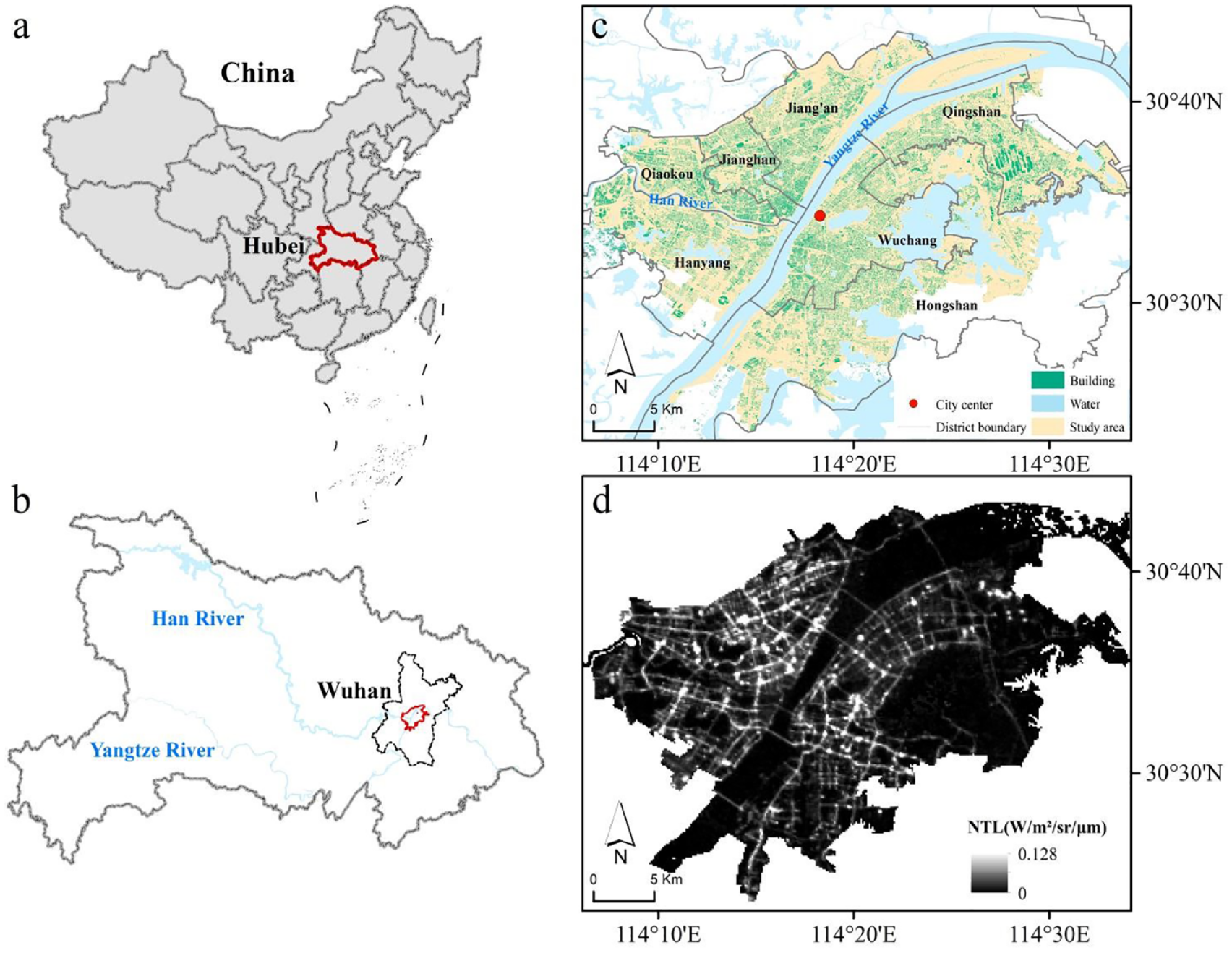
On the left: The location of Hubei province in China (a) and the location of Wuhan in Hubei province (b). On the right: The spatial distribution of buildings and roads in central Wuhan (c) and the spatial distribution of nighttime light in central Wuhan (d).
Data and methods
Data acquisition and processing
The 1:2000 building vector data covering the central urban area of Wuhan in 2018 were provided by Wuhan Geomatics Institute (https://www.whkc.com/), with a position accuracy of 0.2 m. The data contained detailed information about the building footprint, floor number, ground perimeter, and function (Figure 1). We estimated building heights by assuming a floor height of 3.5 m for floors 1 – 6 and 3 m for floors above six, based on the design code for residential buildings in China (GB 50096-2011). To preserve the integrity of buildings as much as possible, we divided the study area into 300 m × 300 m grid units, in which the urban landscape metrics were calculated.
The Luojia1-01 satellite was designed by Wuhan University and launched on 2 June 2018, which provided global NTL imagery with a spatial resolution of 130 m and a temporal resolution of 15 d. We obtained the Luojia1-01 NTL satellite data on 13 June 2018 from Hubei Data and Application Center of High-Resolution Earth Observation System (http://59.175.109.173:8888). A geometric correction was first performed to correct the geo-referencing errors of the NTL data, with utility of the road network data described below (Wei et al., 2017). As the data were stored in integer format, we converted the digital numbers of the original images to NTL radiance as follows :
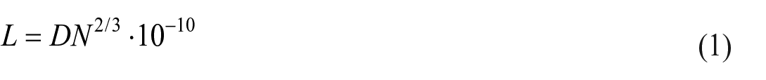
where L is the NTL radiance with the unit of
The road network data relative to 2019 covering Wuhan were produced by Zhou et al. (2022) using the weakly supervised pavement segmentation network. The data had an overall accuracy of 73.59%, which was higher than that of the road network data extracted by conventional methods. It provided multiple information of the road network, including the road type and length. Compared with widely used linear vector road data provided by open street map (OSM), it is polygonal vector data, more convenient for extracting road area information. Considering that the primary sources of road lighting were from street illumination and vehicles, we thereby selected motorways, trunk, primary, secondary, and tertiary roads to obtain road-related indicators.
Calculation of urban landscape metrics
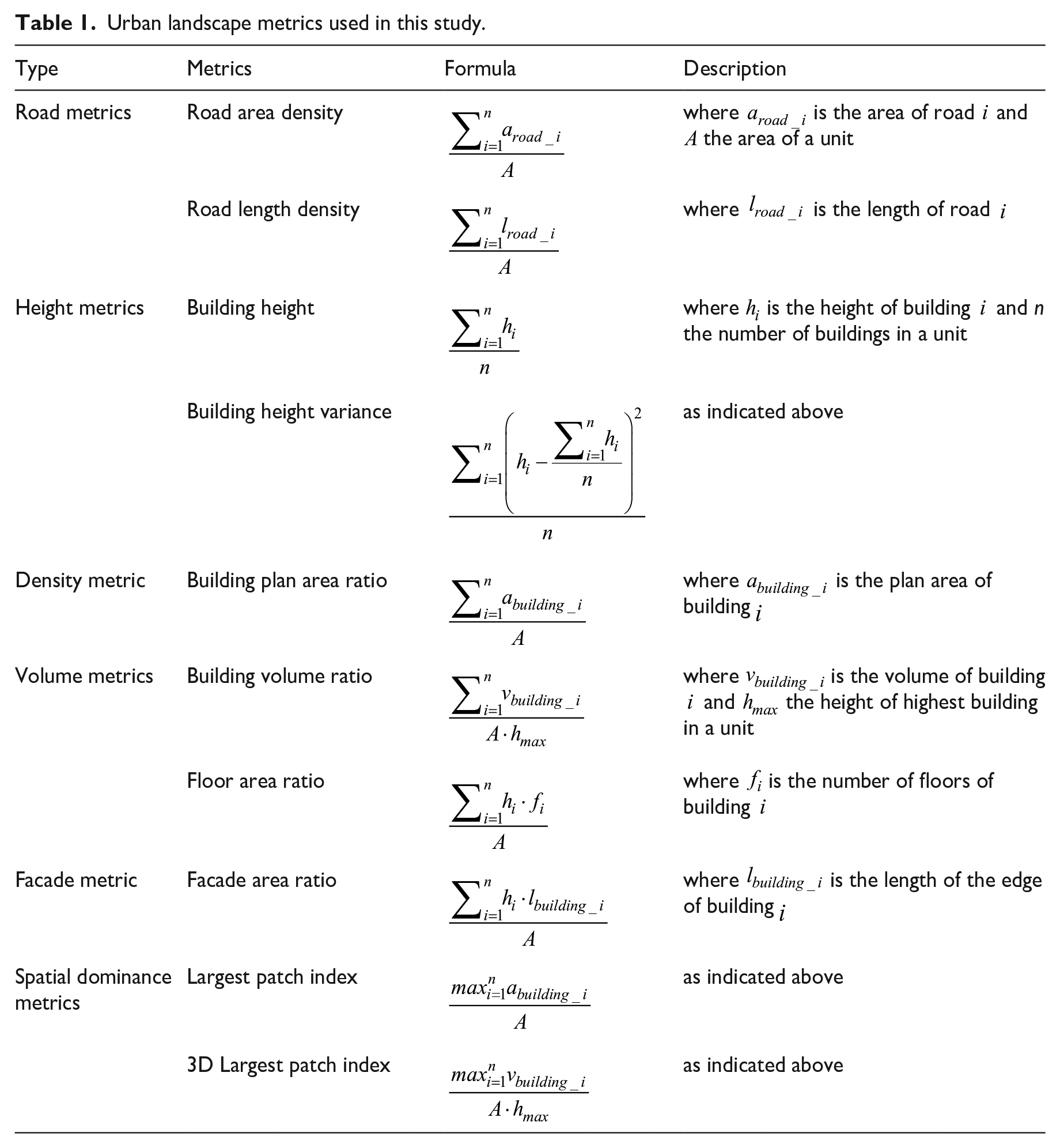
We calculated ten urban landscape metrics based on the 1:2000 building vector data to characterize the urban landscape patterns in central Wuhan. The ten metrics contained two road metrics and eight building metrics. The road metrics signified road lighting and traffic volume, including road area density and road length density. The light intensity of buildings might be influenced by building height, volume, density, as well as the facade of buildings. Therefore, we selected two height metrics, one density metric, two volume metrics, and one facade metric. The height metrics included mean building height and building height variance. The density metric was building plan area ratio. The volume metrics included building volume ratio and floor area ratio. The building volume ratio reflected the efficiency of 3D space utilization in a unit; the floor area ratio reflected the carrying capacity of a unit, referring to the ratio of the gross floor area of a unit to the unit area. The facade area ratio reflected the overall lateral surface areas of all buildings in a unit. The dominant buildings in a unit might also influence its brightness (Wu et al., 2022). Considering this point, we additionally selected two spatial dominance metrics, i.e., largest patch index (LPI) and 3D largest patch index (3d_LPI). The LPI quantified the ratio of the maximum individual building plan area to the unit area, while the 3d_LPI measured the ratio of the maximum individual building volume to the unit volume (i.e., the unit area multiplied by the maximum building height in that unit). The detailed descriptions and calculation formulas of these metrics are presented in Table 1.
Urban landscape metrics used in this study.
Multiscale geographically weighted regression
We used the multiscale geographically weighted regression (MGWR) model to explore the spatial relationships between the urban landscape patterns and NTL intensity in central Wuhan. The MGWR model extended the conventional GWR model by permitting variable-specific bandwidths, thereby accommodating heterogeneous spatial processes operating at distinct scales (Fotheringham et al., 2017). We analyzed the magnitude and direction of different urban landscape metrics’ impact on NTL intensity by examining the correlation coefficients corresponding to them. The MGWR model was formulated as follows:
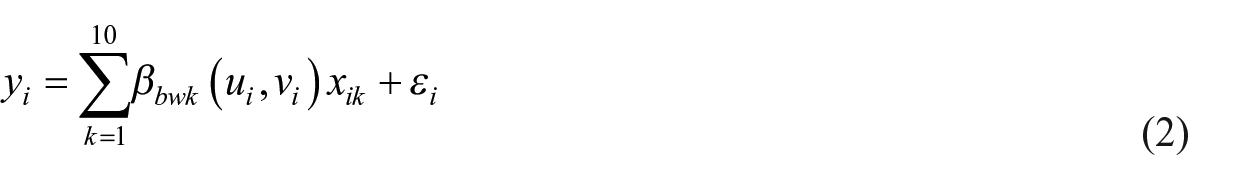
where
Prior to the application of the MGWR model, it was essential to perform diagnostic tests on both the dependent and independent variables to ensure the model’s validity. We first calculated the overall Moran’s I for the NTL intensity to assess the presence of spatial autocorrelation, thereby fulfilling the assumption requirements of the MGWR model. Subsequently, we examined collinearity among all the landscape pattern metrics by identifying the variance inflation factor (VIF), so as to avoid the impact of multicollinearity on the reliability of the model (Dormann et al., 2013). If the VIF of all variables was smaller than 10, there was no significant multicollinearity between the variables. To assess the effectiveness of MGWR, we also employed the GWR model for comparison. The two models were run in the MGWR software version 2.2 developed by Oshan et al. (2019). The performance of the two models was evaluated using the coefficient of determination (R²), adjusted R², Akaike Information Criterion (AIC), and bias-corrected version of AIC (AICc). A lower AIC (and AICc) and a higher R² (and adjusted R²) indicated better model performance.
Extreme gradient boosting model
To relax the assumption of linear relationships in the MGWR model, we also constructed the extreme gradient boosting (XGBoost) regression model to examine the relationships between urban landscape patterns (as independent variables) and NTL intensity (as dependent variable). The XGBoost model was a scalable tree boosting system recognized for its power and efficiency in supervised learning tasks. It was built upon the gradient boosting decision tree algorithm, with enhanced predictive performance iteratively by fitting each new tree to the residuals of the current model predictions (Friedman et al., 2000). The key features of XGBoost included the addition of penalty terms to mitigate overfitting and improve generalization, parallel computation and cache optimization to accelerate data processing efficiency, and capability to manage sparse data and missing values to increase model robustness in practical applications. The datasets that passed the collinearity test were randomly split into a training set (80%) to train the model and a testing set (20%) to evaluate model performance (Chen and Guestrin, 2016; Zhou et al., 2021).
To run the XGBoost regression model, we first tuned eight model parameters, including the number of estimators (ranging from 10 to 100 with an interval of 1), the maximum depth of a tree (ranging from 3 to 10 with an interval of 1), the minimum sum of the weights of all observations in a child tree (ranging from 1 to 6 with an interval of 1), the minimum loss reduction to split a node (ranging from 0 to 0.5 with an interval of 0.1), the sampling rate for each tree (ranging from 0.6 to 0.9 with an interval of 0.1), the sampling rate for columns of each tree (ranging from 0.6 to 0.9 with an interval of 0.1), the learning rate (ranging from 0.05 to 0.3 with an interval of 0.05), and the weight of L1 regularization (equal to 10-5, 10-2, 0.1, 1, or 100). To develop a robust XGBoost model, we initially determined the most crucial parameters (i.e., the number of estimators and the learning rate) while keeping other parameters at their default values. Subsequently, we adopted the grid search method to fine-tune the remaining parameters (Pedregosa et al., 2011). By exhaustively scanning all possible combinations, we identified the optimal set of hyper-parameters based on the R2 of the XGBoost model. Finally, the best regression model was trained using the training datasets to investigate the relationships between urban landscape metrics and NTL intensity.
Shapley additive explanations
Most machine learning models were referred to as ‘black box’ models, as their internal processes for transforming input features into predictions remained opaque to users. However, understanding the model’s decision-making process was as crucial as its construction. In this study, we used the Shapley additive explanations (SHAP) method to explain the outcomes of the XGBoost model, in order to elucidate the contribution of urban landscape patterns to NTL intensity. SHAP was designed for interpretation of machine learning models based on the game theory, which elucidated the model’s decision-making process by evaluating each feature’s contribution according to the SHAP values (Lundberg and Lee, 2017). The sign of the SHAP values (positive or negative) indicated the direction of the landscape patterns’ impact on the prediction results, while the absolute values reflected the strength of the impact. Compared with other similar methods, SHAP provided superior fairness and consistency, and delivered a more robust interpretation of model outcomes from both global and local perspectives.
Based on the SHAP values of the urban landscape metrics, we drew SHAP summary plots, dependence plots, and individual force plots for typical units. The summary plots ranked urban landscape metrics by the mean absolute SHAP values to demonstrate their relative importance. Complemented within the summary plots, the beeswarm patterns provided local interpretation by illustrating the relationships between the feature values and the SHAP values, with color gradients representing the magnitude of feature values. To further elucidate threshold effects, the SHAP dependence plots were drawn to identify critical inflection points where the impact directionality of specific metrics reversed. The force plots quantitatively decomposed model predictions at typical units, employing color-coded bars (red denoting positive contributions and blue indicating negative contributions) with proportional widths reflecting the degree of the impact of urban landscape patterns on NTL intensity, thereby offering granular insights into spatial heterogeneity of driving factors.
Result
Spatial patterns of urban landscapes
The spatial patterns of urban landscapes in central Wuhan relative to 2018 are illustrated in Figure 2. The core urban area around the city center was highly developed. The road area density, road length density, building plan area ratio, floor area ratio, and facade area ratio here were generally higher than other places. This was because the city center featured a mature transportation network with high building density. However, building heights and their variations were relatively small in the city center, due to the presence of historical structures that have existed for centuries. The Qingshan district in the northeastern part of the study area, serves as a major industrial zone, characterized by high building plan area ratio, LPI, and 3d_LPI. In contrast, the road-related indicators, floor area ratio, facade area ratio, and building height variance were relatively low. This was attributed to the prevalence of large low-rise industrial structures and uncomplicated road networks in the area. The building volume ratio showed no obvious regularity in terms of spatial distribution, because it was determined by a complex interplay of multiple factors. Overall, the spatial patterns of urban landscape metrics aligned well with Wuhan’s historical evolution as a metropolis integrating industrial heritage, commercial hubs, and cultural-educational institutions. The complex urban landscape patterns established critical context for subsequent analysis of the human activity-landscape pattern relationships in Wuhan.
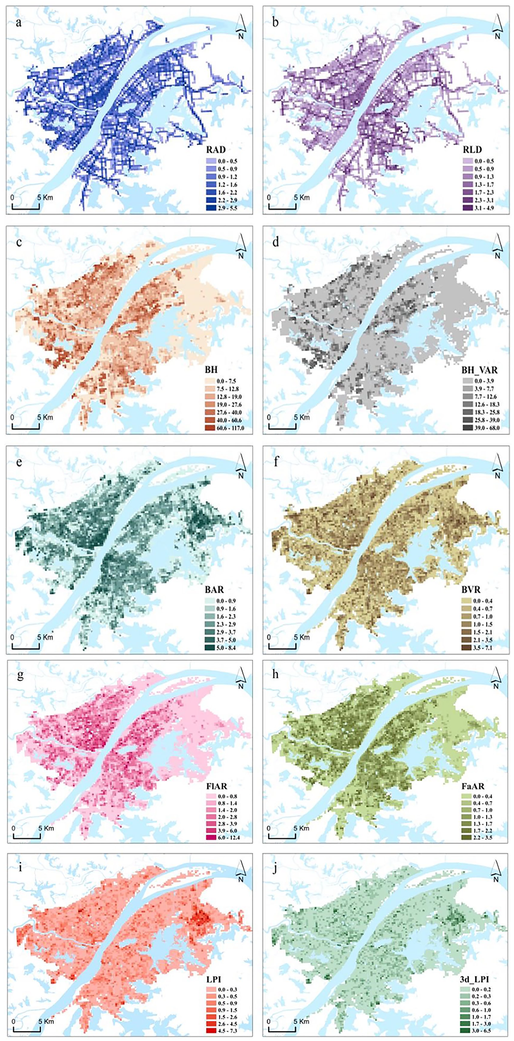
The spatial variability of (a) road area density (RAD), (b) road length density (RLD), (c) building height (BH), (d) building height variance (BH_VAR), (e) building plan area ratio (BAR), (f) building volume ratio (BVR), (g) floor area ratio (FlAR), and (h) facade area ratio (FaAR), (i) largest patch index (LPI), (j) 3d_largest patch index (3d_LPI) in central Wuhan.
Relationships between urban landscape patterns and NTL intensity
As shown in Figure 1d, the NTL intensity exhibited pronounced spatial heterogeneity. The Jianghan, Jiang'an, and Wuchang districts displayed higher NTL intensity, while the Qingshan district, a major industrial zone in Wuhan, showed much lower NTL intensity. The spatial autocorrelation analysis revealed pronounced spatial dependence of the NTL intensity (p less than 0.01, z equal to 76.96, and Moran’s I equal to 0.48). Therefore, we chose local regression models (i.e., GWR and MGWR) instead of global regression models to investigate the relationships between urban landscape metrics and NTL intensity. A collinearity assessment was first performed across all urban landscape metrics to ensure statistical robustness of the models. The diagnostic analyses presented no evidence of multicollinearity among the metrics (Online Supplementary Table S1). The urban landscape metrics were subsequently incorporated into both GWR and MGWR for model comparison. Results showed that MGWR performed better than GWR, with higher R2 and adjusted R2 and lower AIC and AICc (Online Supplementary Table S2). Thus, we applied the MGWR model for the follow-up analysis. Figure 3 showed the relationships between urban landscape metrics and NTL intensity as revealed by the MGWR model. The magnitude and sign of the regression coefficients for a specific urban landscape metric indicated the strength and direction of its effects on the NTL intensity, while the bandwidths represented the spatial range of the local regression for that metric (i.e., how many neighboring observations were included in the local regression; Online Supplementary Table S3). Building height, building plan area ratio, and building volume ratio did not demonstrate statistical significance in the MGWR model, while the remaining seven landscape metrics exhibited significant explanatory power at the 95% confidence level.
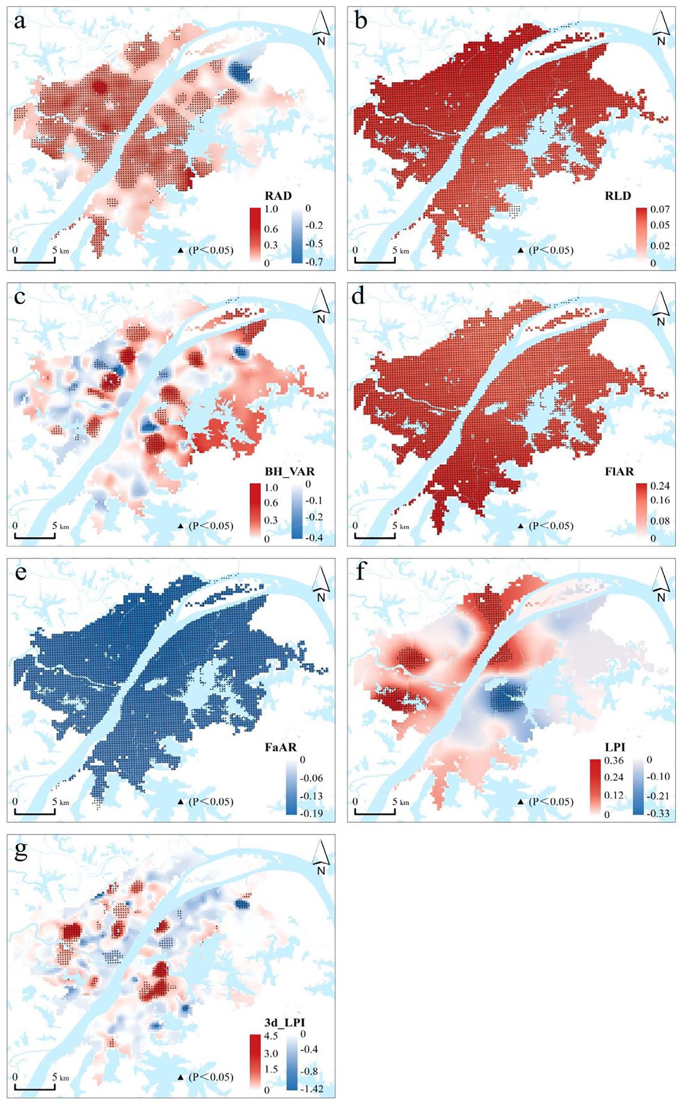
The local regression coefficients of MGWR between the urban landscape metrics and NTL intensity: (a) road area density (RAD), (b) road length density (RLD), (c) building height variance (BH_VAR), (d) floor area ratio (FlAR), (e) facade area ratio (FaAR), (f) largest patch index (LPI), and (g) 3D largest patch index (3d_LPI).
Specifically, road length density, floor area ratio, and facade area ratio exhibited globally consistent effects on the NTL intensity. However, the regression coefficients for road length density were very low (less than 0.1), indicating that it was not a key influencing factor. Floor area ratio had a positive effect on the NTL intensity (with the maximum coefficient equal to 0.24), whereas facade area ratio had a negative effect (with the minimum coefficient equal to -0.19). The road area density showed a positive correlation with the NTL intensity across most locales, with the maximum coefficient up to 1.0. Exception existed in a small area located in the Qingshan district, where a significant negative correlation was found. The effects of building height variance on the NTL intensity were localized. Clearly, partial areas along the Yangtze River displayed a significant positive correlation, with the regression coefficients as high as 1.0. In contrast, some locales, e.g., in the Qingshan district, showed a negative correlation with the coefficients more than -0.4. In terms of the spatial dominance metrics, 3d_LPI had the largest coefficient values among all the seven metrics, ranging between -1.42 – 4.5. Significant positive correlations were widely distributed while negative correlations also existed in some locales. LPI exerted a dominant positive effect on the NTL intensity on the western bank of the Yangtze River, while a dominant negative effect was found on the eastern bank, with the regression coefficients ranging between -0.33 – 0.36.
We also identified the two most influential factors of the NTL intensity in each unit by comparing the absolute values of the regression coefficients derived from the MGWR model. As illustrated in Figure 4a, areas with floor area ratio and road area density as the primary influential factors accounted for the largest proportion, equal to 54.95% and 31.67% respectively. Obviously, areas with road area density as the primary driver were concentrated in the urban core around the city center, while those with floor area ratio as the primary driver distributed in the northern and southern portions of the study area. Locales with 3d_LPI, building height variance, and LPI as the primary influential factors accounted for a small portion, equal to 7.45%, 5.28%, and 0.65% respectively. In areas with road area density as the primary influential factor, the secondary one was predominantly floor area ratio. In areas with floor area ratio as the primary one, facade area ratio emerged as the secondary one. In locales with 3d_LPI as the primary key landscape metric, road area density emerged as the secondary one. Additionally, in locales with building height variance as the primary influential factor, floor area ratio emerged as the secondary one.
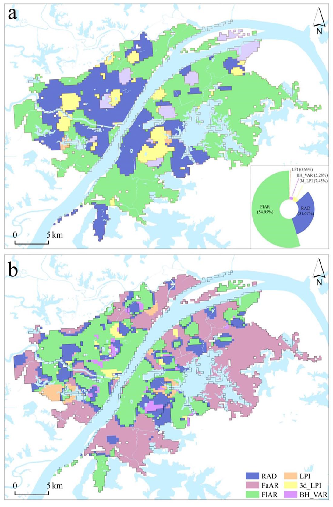
The primary (a) and secondary (b) key urban landscape metrics influencing the NTL intensity in central Wuhan.
Contributions of urban landscape metrics to NTL intensity
To relax the linear assumption in the MGWR model, we constructed an XGBoost regression model to investigate the non-linear relationships between urban landscape patterns and NTL intensity, if any. The hyperparameter tuning was conducted via a grid search approach, and the optimal combination of the eight key hyperparameters are presented in Online Supplementary Table S4. We also employed the SHAP method for interpreting the outputs of the XGBoost model. The mean of absolute SHAP values was calculated to assess the relative importance of different metrics on NTL intensity (Figure 5a). Road area density was the most important metric influencing the NTL intensity globally (with the mean absolute SHAP value equal to 3.4), followed by floor area ratio (equal to 2.7), building height variance (equal to 1.8), and road length density (equal to 1.7). In contrast, building height, building volume ratio, and building plan area ratio had the lowest SHAP values (less than 0.5), indicating a minimal impact on the NTL intensity (which were excluded from the following analysis). This was generally consistent with the results derived from the MGWR model, except that road length density exhibited a higher level of importance. In addition to the absolute SHAP values, the color-coded beeswarm plots were drawn to visualize the macroscopic relationships between the SHAP values and the magnitude of feature values, which also revealed the directional effects of urban landscape metrics on NTL intensity (Figure 5b). Results showed that the relationships between urban landscape metrics and NTL intensity were not unidirectional. Overall, high feature values (represented in red) were predominantly clustered on the right side of the zero axis, correlating with positive effects, while lower feature values (in blue) were countertraded on the right side, associated with negative effects. This pattern was reversed for facade area ratios, which showed an opposite distribution trend compared with other metrics.
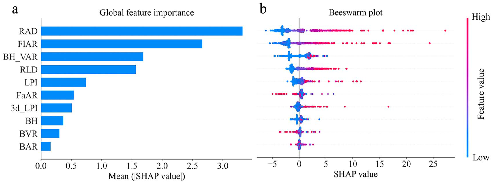
The SHAP analysis to interpret prediction results of the XGBoost regression model: (a) global feature importance and (b) beeswarm plot.
As a complement to the beeswarm plots, the SHAP dependence plots were drawn to show how the effect of urban landscape patterns on NTL intensity varied as their feature values changed, and explicitly identify critical inflection points where the effect directionality reversed (Figure 6). For road area density, when the feature values were below the critical threshold (approximately 0.1), it exhibited a negative effect on the NTL intensity. Once the threshold was exceeded, the effect was turned into a positive, and the SHAP values increased sharply as the feature values enlarged, indicating an intensification of such effect. Floor area ratio, as well as road length density, showed a similar dependence trend. For building height variance, the SHAP values slowly increased with the higher feature values and soon plateaued as the feature values approached 2000. For facade area ratio, the SHAP values remained positive and stable if the feature values ranged between 0 – 1.5, and were turned into a negative once the feature values exceeded 1.5. In addition, this metric exerted the minimal influence on the NTL intensity among all the examined metrics, with its SHAP values clustering near the zero axis throughout the entire range of feature values. The feature values of LPI and 3d_LPI both exhibited positive correlations with their SHAP values. The data points had highly concentrated distributions but with two outlier clusters: data points with high feature values but low SHAP values and those with low or moderate feature values but high SHAP values. Overall, this nonlinear response contrasted with the unidirectionality identified by the MGWR model, in which road length density, floor area ratio, and facade area ratio exerted a consistently global effect across all units.
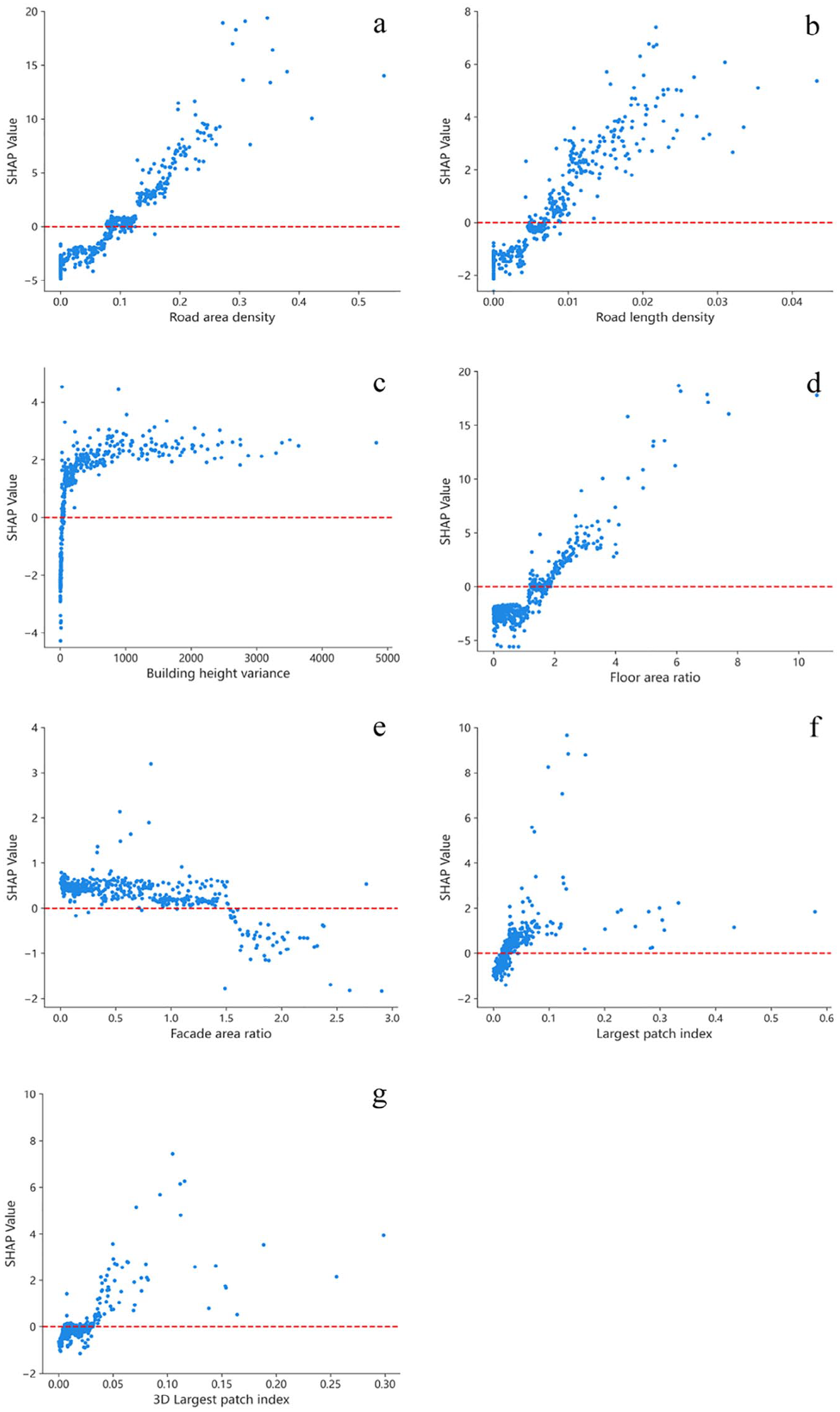
The SHAP dependence plots of the urban landscape metrics: (a) road area density, (b) road length density, (c) building height variance, (d) floor area ratio, (e) facade area ratio, (f) largest patch index, and (g) 3d_largest patch index.
Local interpretability analysis of typical plots
We finally selected four typical plots with commercial, industrial, historic, and educational functions to understand how the driving landscape metrics influencing the NTL intensity varied in different urban function zones. Plot A was Wuhan Tiandi, one of the most prosperous commercial centers in Wuhan (Figure 7a). The SHAP force plot revealed that road area density, road length density, floor area ratio were the primary drivers with positive effects, whereas building volume ratio and building plan area ratio showed weak negative effects. Plot B was Wuhan Iron and Steel Company located in the industrial zone, which was characterized by large low-rise factorial structures (Figure 7b). As a consequence, the NTL intensity was positively influenced by 3d_LPI, building height variance, and LPI but negatively influenced by floor area ratio, road area density, and road length density. Plot C enclosed parts of the Jianghan Road with significant commercial and cultural attributes (Figure 7c). Floor area ratio and road length density were the primary driving metrics positively influencing the NTL intensity, whereas road area density and facade area ratio were identified as key negative drivers. Compared with plot A, road length density showed a positive effect while road area density showed a negative effect in plot C. Plot D was the gymnasium of Wuhan University, representing educational land use (Figure 7d). The NTL intensity was primarily enhanced by LPI whereas road area density was the main negative suppressor. Compared with plot B, only the influence of LPI was highlighted in plot D, with 3d_LPI playing a less important role.
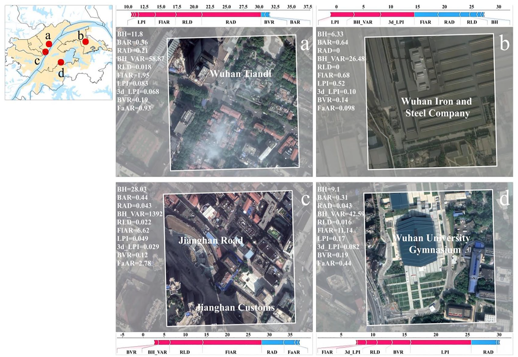
The SHAP force plots for typical plots: (a) Wuhan Tiandi, (b) Wuhan Iron and Steel Company, (c) the Jianghan road, and (d) the gymnasium of Wuhan University.
Discussion
This study explored the relationships between urban landscape patterns and human activity intensity in Wuhan, using the NTL data as a proxy. As global regression models have estimation bias and limited capacity to handle multidimensional data, we adopted a local regression model (i.e., MGWR) which incorporated spatial dependence information. Results showed that road area density and floor area ratio were the most two important metrics influencing the NTL intensity, while 3d_LPI, building height variance, and LPI had significant localized effects. To validate the results derived from MGWR with an inherent linear assumption, we further utilized a machine learning model (i.e., XGBoost) to analyze the relationships between urban landscape patterns and NTL intensity based on non-linear assumption. Comparison between the two distinct kinds of models demonstrated high consistency in terms of the influencing factors. Both marginalized the contributions of building volume ratio, building plan area ratio, and building height, and identified road area density and floor area ratio as the primary key metrics influencing the NTL intensity. In addition, the MGWR model identified the dominant influence of LPI and 3d_LPI in certain locales, which was consistent with the prediction of the XGBoost model in some educational and industrial units occupied by large low-rise structures.
Higher road area density usually corresponded to greater traffic flow and more road lighting, making it the dominant factor affecting NTL intensity in area with complex road networks (Chang et al., 2020). Floor area ratio was a crucial urban planning metric, with higher floor area ratio indicating higher load capacity and intensified human activities. Hence, floor area ratio was also a key explanatory variable affecting NTL intensity (Lin et al., 2023). In contrast to the comprehensiveness of floor area ratio in capturing urban structures, building height and building plan area ratio offered limited, unidimensional perspectives on building characteristics, thus resulting in negligible influence on NTL intensity (Wang et al., 2019). Although building volume ratio was also an indicator encompassing both building height and density characteristics, its measurement was constrained by the maximum building height within the spatial unit of analysis. As a result, building volume ratio showed low spatial heterogeneity, thereby weakening its impact on the spatial variability of NTL intensity. Overall, road area density was the most significant determinant of NTL intensity in the well-developed road networks of the central sector, whereas floor area ratio dominated in the northern and southern portions of the study area. For LPI and 3d_LPI, their influence on NTL intensity was primarily manifested in spatial units dominated by large-scale building entities, which was consistent with previous research (Wu et al., 2022).
Notable exceptions were observed for road length density and facade area ratio. While the MGWR model revealed that road length density had a globally positive yet negligible effect (with minimal regression coefficients) on NTL intensity, its importance increased substantially in the XGBoost model. Meanwhile, façade area ratio exhibited a global negative effect in MGWR but demonstrated clear bidirectional influences in XGBoost. This discrepancy originated from the strategies employed by the two models to measure the degree of influence of variables. First, the MGWR model employed linear fitting, with the regression slopes representing each variable’s influence strength (Fotheringham et al., 2017). This might underestimate the contribution of outliers to the prediction results. In contrast, the SHAP method measured marginal contributions across all possible feature combinations, providing a more comprehensive evaluation of feature contributions (Lundberg and Lee, 2017). Second, the large bandwidths estimated for some independent variables in MGWR might mask threshold effects where the sign of independent variables exhibited directional reversals. In contrast, the tree-based architecture of XGBoost accommodated threshold effects, allowing variables to exhibit opposing influences across different value ranges (Chen and Guestrin, 2016). Nevertheless, the overall high consistency between the two distinct models in this study suggested that simple non-linear relationships predominantly characterized the associations between urban landscape patterns and NTL intensity. Otherwise, the MGWR model might produce large bias (Li, 2022; Okumus and Akay, 2025). It should also be noted that the XGBoost model did not consider spatial autocorrelation, which might generate spurious correlations (i.e., erroneously attributing geographical contextual effects to clustered variables in a region).
In terms of the effect of facade area ratio on the NTL intensity, we found that low facade area ratio in our study area corresponded with mixed land use (e.g., combination of commercial and official functions) and high NTL intensity, whereas high facade area ratio (>1.5) corresponded with single-function structures (primarily residential buildings) and lower human activity intensity (Li et al., 2022; Lu et al., 2019). The XGBoost model also identified distinct impacts of the same landscape metric on NTL intensity across spatial units with different functional types. For example, the NTL intensity in the commercial unit favored both road area and length density, while that of the historical unit with commercial function only favored road length density. This was because the historical unit restricted vehicle traffic and primarily allowed for the presence of pedestrian roads. Likewise, the educational unit only highlighted the strong influence of LPI on the NTL intensity, while the industrial unit highlighted the influence of both LPI and 3d_LPI. This was primarily because the industrial unit had a limited number of buildings with small building height variations. Therefore, the 3d_LPI could well represent the characteristics of the dominant building in the unit. However, in the more complex built environment such as the educational unit, the LPI was a better indicator as it was only determined by the plan area of the largest building and the unit area.
This study, with utility of both the MGWR and XGBoost models, provided an innovative perspective for understanding the relationships between urban landscape patterns and human activity intensity. However, it could be further explored in several ways. First, the seasonal effects of urban landscape patterns of NTL intensity should be highlighted. As a crucial proxy indicator in urban studies, high spatiotemporal resolution and long-term time-series NTL data are still lacking (Chen et al., 2019; Lan et al., 2020). In this study, we selected the Luojia1-01 NTL data on 13 June 2018 to conduct our research due to data availability. However, the effects of urban landscape patterns on NTL intensity might vary across different seasons because human activities exhibit seasonal patterns. Second, the effects of other influencing factors on NTL intensity should also be considered. Our study mainly focused on the effect of urban landscape patterns. The explanatory power (R2) of the selected urban landscape metrics for NTL intensity was 0.51, which fell within the reasonable range but with moderate level compared with other relevant studies (generally between 0.3 and 0.8; Lu et al., 2019; Wu et al., 2022). This indicated that the NTL intensity was influenced by other factors, such as population and economy (Zhao et al., 2019; Zheng et al., 2023). Therefore, future studies could benefit from a more comprehensive selection of indicators to holistically examine the driving force of human activity intensity, using NTL data as a proxy, across multiple spatiotemporal scales.
Conclusion
This study explored the relationships between urban landscape patterns and human activity intensity in Wuhan, using NTL data as a proxy. To validate the relationships, the MGWR and XGBoost models with distinct assumptions were both applied. The prediction results of XGBoost corresponded closely with those derived from MGWR. Both models confirmed that road area density and floor area ratio exerted the most substantial influence, while building height, building plan area ratio, and building volume ratio had minimal effects. Additionally, the same landscape metric had a distinct impact on NTL intensity across spatial units. Discrepancies were also found between the two models, e.g., regarding the importance level and directionality of effects for metrics including facade area ratio and road length density. The discrepancies primarily stemmed from MGWR’s linear assumption, which overlooked information contained in partial outlier data points and neglected the threshold effects particularly when the independent variables were associated with large bandwidths. Our study demonstrated that the XGBoost model better approximated the authentic relationships between urban landscape patterns and NTL intensity. Future studies should investigate the seasonal dynamics between urban landscape patterns and human activity intensity, while integrating additional contextual factors to enable more comprehensive assessments.
Supplemental Material
sj-docx-1-tee-10.1177_2754124X251336970 – Supplemental material for Are urban landscape patterns associated with human activity intensity? Evidence from nighttime light data
Supplemental material, sj-docx-1-tee-10.1177_2754124X251336970 for Are urban landscape patterns associated with human activity intensity? Evidence from nighttime light data by Shengyuan Dong, Qian Cao, Lunche Wang, Baojie He and Ruimin Fang in Transactions in Earth, Environment, and Sustainability
Footnotes
Declaration of conflicting interests
The author(s) declared no potential conflicts of interest with respect to the research, authorship, and/or publication of this article.
Funding
The author(s) disclosed receipt of the following financial support for the research, authorship, and/or publication of this article: This study was supported by the National Natural Science Foundation of China (No. 42371115).
Supplemental material
Supplemental material for this article is available online.
Author biographies
References
Supplementary Material
Please find the following supplemental material available below.
For Open Access articles published under a Creative Commons License, all supplemental material carries the same license as the article it is associated with.
For non-Open Access articles published, all supplemental material carries a non-exclusive license, and permission requests for re-use of supplemental material or any part of supplemental material shall be sent directly to the copyright owner as specified in the copyright notice associated with the article.