
Abstract
This study evaluates the potential of market-available crowdsourced driving data—connected vehicle (CV) data in estimating crossing times for passenger vehicles at ports of entry (POEs). Two months of CV data collected from a POE at the US-Mexico border in El Paso, Texas were processed using cloud computation tools to generate hourly aggregated border crossing times (CV-Time). In addition, this study also generated different variables to characterize the speed profile of CVs at different locations along a POE. Different regression models were developed to estimate border crossing times based on CV-generated variables and compared with ground truth observations from existing monitoring systems. The results show that the CV-Time is strongly correlated with the ground truth observations with a correlation rate of 0.82. The best-fitted Gradient Boost Regression model achieved an RMSE of 15.50 and MAPE of 25%. Our findings suggest that market-available CV data is promising for monitoring border crossing times, especially for supplementing physical monitoring systems when they are down for maintenance.
Introduction
Traffic congestion is a growing problem in many cities worldwide, which refers to the situation where the volume of vehicles on a portion of roadway exceeds its capacity, resulting in slower speeds, longer travel times, and higher vehicle emissions. It has been recognized as a long-standing transportation issue, especially in land ports of entry (POEs), where security inspections or other procedures are performed on vehicles and passengers to ensure homeland security but this leads to spillover effects such as increased border crossing time (Lin et al., 2014; Roberts et al., 2014). Border delays have significant impacts on various aspects of society. Increased crossing times at border crossings can negatively impact the economy, particularly for businesses that rely on the timely delivery of goods. It also increases time and cost of delivering goods to consumers (McCord et al., 2016; Roberts et al., 2014). For example, as one of the longest international borders in the world, the United States (US) and Mexico share a border of almost 2,000 miles with 44 border crossings, where delays at US-Mexico crossings resulted in a $7.8 billion economic cost in 2011 (Biery, 2013). Driven by the exponential trade growth between the United States and Mexico, especially with the United States–Mexico–Canada Trade Agreement entered into force, the transportation efficiency at border crossings is facing greater challenges. Meanwhile, congestion at POEs can negatively impact the environment. Idling vehicles waiting to cross the border can produce up to twice the carbon emissions, which can harm both the environment and human health in border communities (Khan, 2010). Therefore, effective monitoring border crossing times is essential for border crossing management and planning purposes and can also support a variety of needs (e.g., when and where to cross the border) of border commuters, travelers, and private-sector business (The San Diego Association of Governments, 2017). However, current measurement solutions usually require a large installed base of sensors (e.g., Bluetooth/Wi-Fi readers), which are costly to implement and maintain. Effectively and cost-efficiently monitoring passing vehicles’ crossing times at POEs remains a challenging problem.
Recent advancements in the Internet of Things (IoT) technology have led to the emergence of various mobility data sources that can effectively track the movements of a large number of vehicles, paving a new avenue for more efficient solutions to monitor the crossing times of vehicles at POEs. As one of the most promising examples fueled by IoT technologies, connected vehicles (CVs) are gradually becoming the new paradigm of road transport, with the ability to positively influence transportation safety, efficiency, and sustainability. CVs represent the unification of various connectivity technologies, enabling vehicles to communicate with other vehicles (V2V), transportation infrastructures (V2I), and the cloud (V2C) to achieve the goal of self-driving (Hoseinzadeh et al., 2020; Talebpour and Mahmassani, 2016). While most commercially available vehicles are still not fully automated with limited communication functions, they can monitor the driving environment and vehicle movements through vehicular sensors. Many world-leading auto manufacturers, like Toyota™, General Motors™, BMW™, and Tesla™, have ramped up production of CVs that can access and transmit vehicular sensors’ data to the cloud (Miles 2019). Many automotive data companies like Wejo, Otonomo, Smartcar, Vinili, and CarAlgo have emerged to bridge the gap between data providers (auto manufacturers) and data users by ingesting, aggregating, and normalizing mobility data from millions of V2C vehicles and delivering the enriched and organized datasets to end users (Miles 2019). CV datasets from commercial data suppliers have shown great superiority in data quality, volume, consistency, and richness compared to traditional mobility data sources, making it a promising data source for monitoring mobility dynamics (Li et al., 2021). However, whether and to what extent the market-available CV data could be implemented in border crossing estimation is still underexplored, which requires further investigation.
This study aims to explore the potential of this emerging crowdsourced mobility data—market-available CV data to estimate crossing times for passenger vehicles at POEs. We made use of the CV data obtained from a commercial CV data provider and replicated the calculation procedure of existing Bluetooth-based systems to calculate the hourly aggregated border crossing times based on the CV data (CV-Time). Meanwhile, we also generated a set of variables to characterize the speed profile of vehicles at different locations along a POE. Finally, we developed different regression models to estimate the border crossing times based on CV-generated variables and statistically compared them with the ground truth observations from existing border time monitoring systems. Some preliminary findings of this work have been published to introduce this new data (Jalilifar et al., 2022). However, this study differs from our previous paper in several significant ways. First, data collection period has been extended from one week to two months to improve the reliability of the results. Second, we have introduced twenty-two additional variables to capture the dynamics of driving speed and differentiate rush-hour and weekend traffic flows. Finally, we have created and compared different regression models to optimize the modelling results. Through this data-driven practice, we aim to help transportation and planning agencies, such as the federal and state departments of transportation (DOTs) and Metropolitan Planning Organizations (MPOs), better assess traffic conditions and effectively recognize highly congested roadway segments.
Literature review
For a considerable time, the United States Customs and Border Protection (CBP) has been the primary provider of crossing times at the US POEs, which is estimated through three main solutions: unaided visual observation, camera snapshots, and driver surveys (Villa et al., 2017). However, these estimates require a significant amount of human input and are unreliable with limited samples (Rajbhandari and Villa, 2012). Recently, new techniques have been adopted to monitor crossing times at POEs. In general, there are three commonly used methods to estimate border crossing times: queue length detection, fixed point vehicle reidentification, and dynamic vehicle tracking (Rajbhandari et al., 2012a; The San Diego Association of Governments, 2017). Queue length detection measures the arrival and departure rates of vehicles and calibrates models to estimate queue end. Fixed-point vehicle reidentification calculates the time spent by a vehicle traveling between two fixed points. Dynamic vehicle tracking uses wireless signals emitted by devices placed in vehicles to estimate time spent at a given spot or between various locations. However, these solutions require a large installed base of sensors, which are costly to implement and maintain (Khan, 2010; Rajbhandari et al., 2012b; Ramezani and Geroliminis, 2015).
With the advent of mobile sensing and the maturation of IoT technology, crowdsourced traffic data are becoming a promising option in transportation monitoring and management (An et al., 2016; Guo et al., 2016; Li and Goldberg, 2018; Li et al., 2019). For travel time data collection, crowdsourced methods are among the most used private-sector mechanisms today. Mobile devices carried by drivers or installed in their vehicles can provide detailed information about their location, speed, and possibly additional information to a public or private entity, which can then be used to generate traffic/travel time information (The San Diego Association of Governments, 2017). For example, Waze, as a leading crowdsourcing mobile app, has been used to monitor traffic conditions (Li et al., 2020). Additionally, several mobile apps, such as Toronto Buffalo Border Wait Time (TBBW), Border Wait Times, and Best Time to Cross Border, have been developed to gather border wait times from users (Lin et al., 2015). Compared to mobile devices, CV represents a more transformative crowdsourced data source for monitoring the mobility dynamics of vehicles (Li et al., 2021). The Texas A&M Transportation Institute (TTI) conducted a comparison of different emerging data sources for crossing time estimation and found that CV technology provides the highest value for the enhanced border crossing time measurement system (Villa et al., 2017). Although CV-related technologies are still in the early stages of development, they have been prototyped and tested for several decades and hold great promise (The San Diego Association of Governments, 2017). However, to the best of our knowledge, there is no dedicated study to investigate whether and how market-available CV data can be used in congestion studies in areas typically lacking data, such as border crossings. This study attempts to fill in this knowledge gap by conducting a pilot study to assess the potential of the market-available CV data in border crossing time estimation.
Study area and data sources
This study compared two months (September and October 2022) of market-available CV data with the border crossing times retrieved from the existing border crossing information system (BCIS) for passenger vehicles at the Paso del Norte (PDN) International Bridge in El Paso, Texas. Please note that the “ground truth” estimates from the BCIS system represent the average crossing times for all vehicles within a one-hour interval. To ensure a fair and accurate comparison, we opted to use the same interval when generating estimates based on the CV data.
Study site—PDN International Bridge
The PDN International Bridge is one of the busiest POEs in the United States, located at 1000 S. El Paso Street on the United States side and on Juárez Avenue on the Mexican side. Operating 24 hours a day, seven days a week, it is dedicated to pedestrians (northbound and southbound) and passenger vehicles (northbound), with over 10 million people traveling from Mexico to the United States annually at this location (Sharma et al., 2018). As the CV data examined in this study are collected specifically from the passenger vehicles, the PDN POE is an ideal study site to evaluate the effectiveness of this data in border crossing time estimation.
Data source
We first collected border crossing times from the existing Border Crossing Information System (BCIS) (https://bcis.tti.tamu.edu/), developed and maintained by the Texas A&M Transportation Institute for monitoring the travel times of passenger vehicles crossing the United States and Mexico border. The BCIS is based on a reidentification approach using Bluetooth readers (Readers) at passenger vehicle POEs, which captures mobile devices’ signals (Bluetooth media access control [MAC] address) carried by vehicles, drivers, or passengers at multiple locations along the path for each border-crossing trip.
Border crossing time is usually defined as the time it takes, in minutes, for a vehicle to reach the United States CBP’s primary inspection booth after arriving at the end of the queue (Sharma et al., 2018; Texas A&M Transportation Institute, 2023). This queue length varies and depends on traffic volumes and processing times at each of the inspection facilities throughout the border crossing process. The variable nature of the queue makes the installation location of Readers critical. Five Bluetooth readers were installed along the PDN POE, labelled as Reader 1–5. Since the queue of vehicles at the PDN POE usually can reach as far as Reader 1, as illustrated in Figure 1, this study defines the border crossing time as the time a vehicle takes, in minutes, to travel from Reader 1 to Reader 5. Reader 1 was installed near the intersection of Juárez Avenue and 16 de Septiembre Street, representing the starting point to observe the queue. Reader 5 was installed at the United States CBP inspection facility.
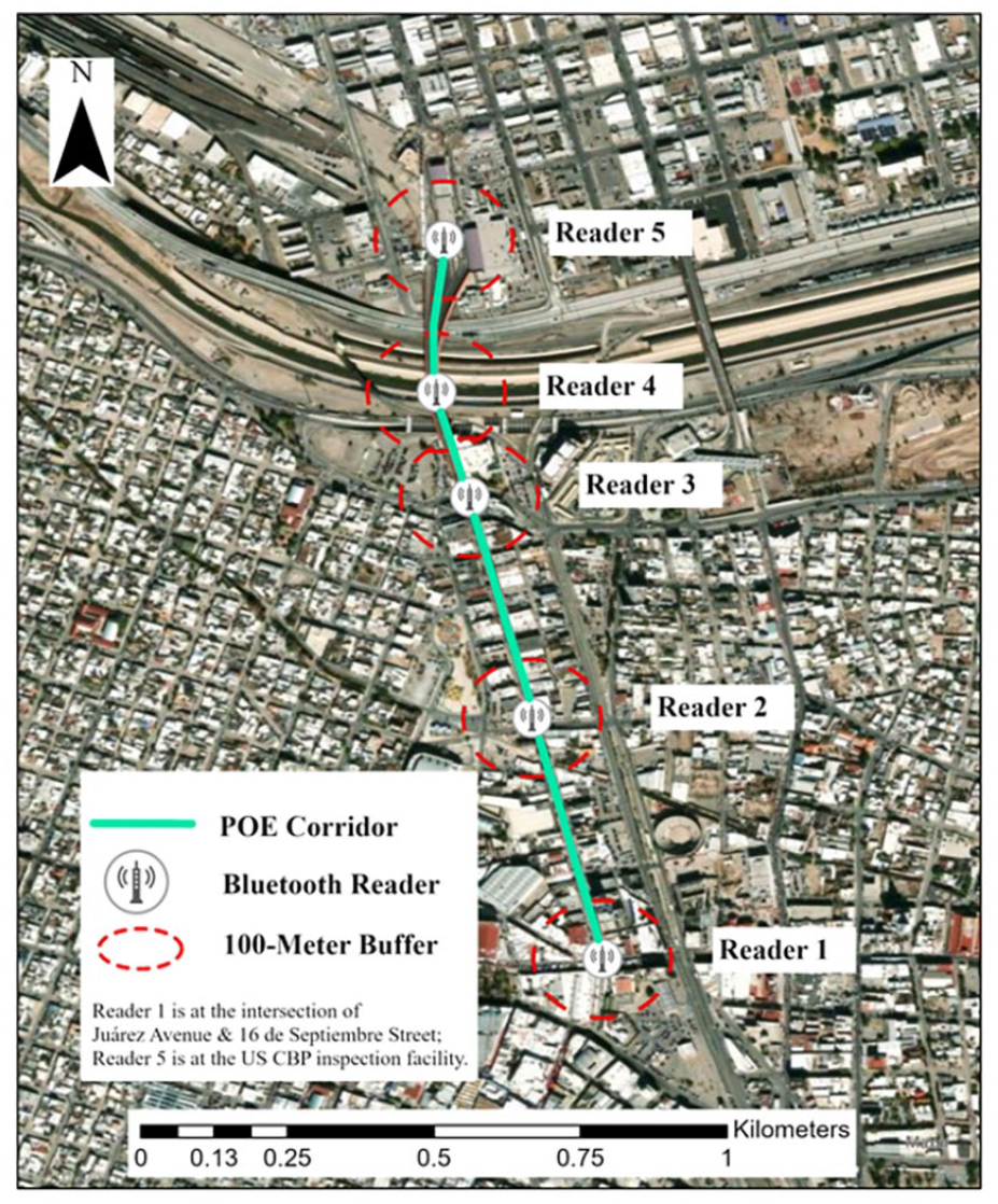
The distribution of five installed Bluetooth readers along the PDN POE.
For CV data, this study used two months of CV data (September and October 2022) provided by a commercial CV data start-up, which provides high sampling rates and multi-dimensional vehicle movements and driving events (e.g., hard braking, hard acceleration, and speeding) data. This data platform has partnered with multiple world-leading auto manufacturers and collected data from millions of V2C vehicles with a sampling rate of three seconds per waypoint. Each waypoint describes the timestamp, location, and movement-related information (e.g., speed and heading) of a vehicle’s trajectory (Li et al., 2021). This study used the border crossing trajectory data collected from CVs to estimate border crossing times at PDN POE.
Methodology
Figure 2 illustrates the research workflow of this study. Two datasets were used, including border crossing times obtained from the current BCIS at the PDN POE and the CV data. Responding to the inherent big-data nature of the CV data, we utilized a set of cloud-based big data analytics tools to store, manage, and process the CV data. We then generated the border crossing time estimates based on the CV data (CV-Time) by replicating the calculation procedure of the BCIS. Additionally, we created a set of new variables to capture the traffic volume and speed variances of CVs at different locations along the corridor to the PDN POE. We built different regression models to estimate border crossing times based on the CV-Time and CV-based additional variables. Finally, we compared the raw CV-Time (without modelling) and the modelled CV-Time (after modelling) with the ground truth to assess their similarities and make recommendations on how to use market-available CV data for border crossing time management.
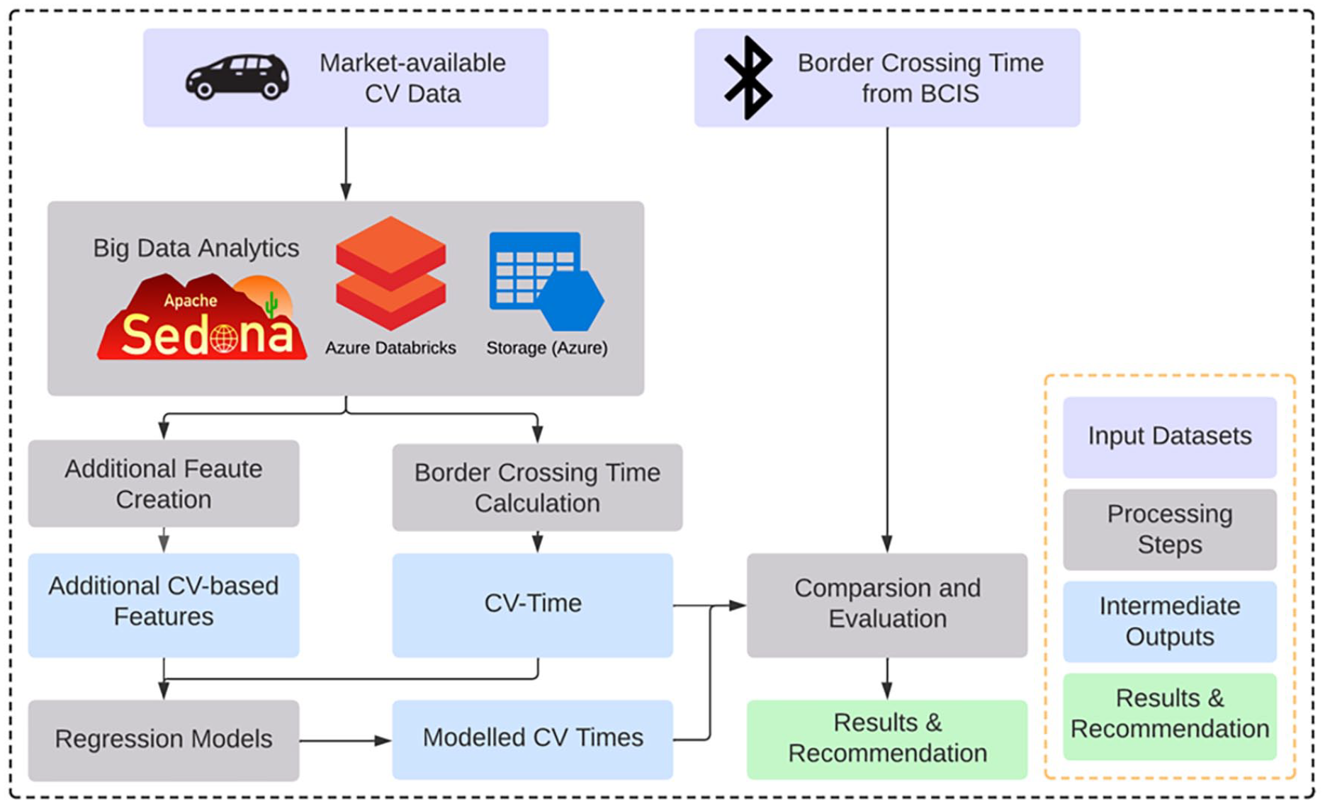
Research workflow.
Big data analytics tools for processing CV data
As mentioned above, the CV data were collected from millions of vehicles at a high sampling rate, resulting in terabyte-level datasets. For example, the two-month CV data for Texas is around four terabytes. Therefore, cloud-based big data analytics tools were needed to store, manage, and process this dataset. In this study, we utilized Microsoft Azure Cloud Storage to store the CV data (Copeland et al., 2015). The original CV data were organized in the Apache Parquet format. For effectively manipulating the data, we used an online big data analytics platform, Azure Databricks, to process the big CV dataset. Azure Databricks supports the latest version of Apache Spark, allowing its users to seamlessly integrate with any open-source libraries and quickly establish a fully managed Apache Spark environment. We primarily used Apache Sedona and H3 spatial indexing system to load, partition, process, and spatially analyze the big CV data. By taking advantage of these big data analytics tools, this study subset the state-wide CV dataset to cover the border crossing regions at the PDN POE.
Border crossing time calculation
As mentioned before, the BCIS at the PDN POE consists of five Bluetooth readers installed at different key locations. That is to say, for each trip, the vehicle could be captured at multiple locations. By matching the captured Bluetooth MAC addresses at different pairs of Bluetooth readers, we could obtain the vehicle’s travel times crossing different monitored segments based on the captured timestamps, as illustrated in Figure 3. For example, the hourly average travel time of the segment (SegTime) from an entering reader (Reader 1) to an exiting reader (Reader 2) can be calculated using Equation 1:
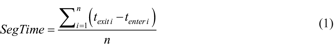
where
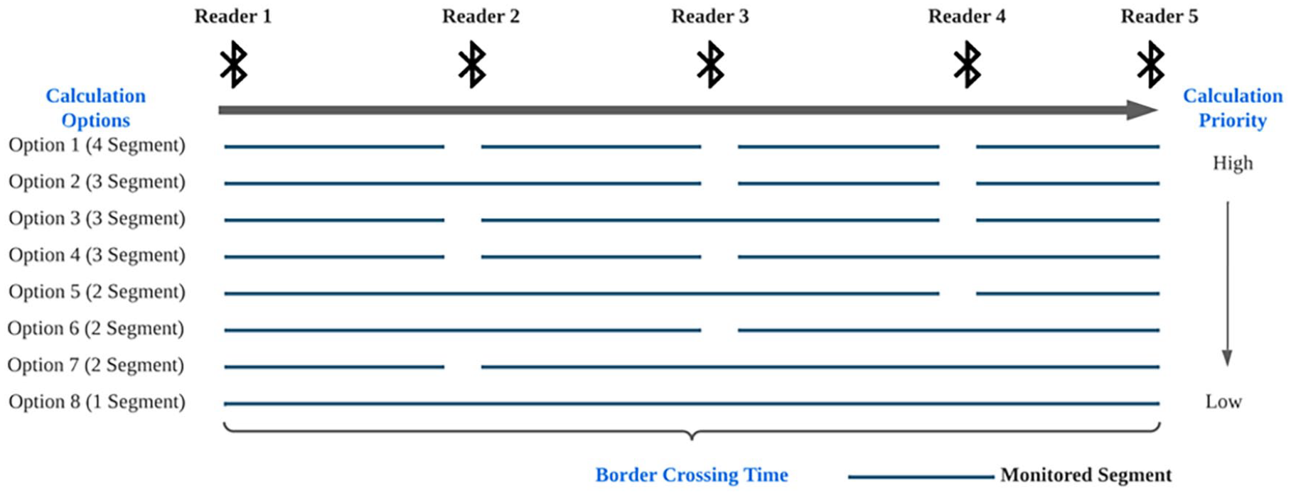
Illustration of border crossing time estimation.
To calculate the hourly average border crossing times at the PDN POE, we need to determine how to aggregate the hourly average travel times on different monitored segments into a single border crossing time from Reader 1 to Reader 5. As shown in Figure 3, there are eight different calculation options to form a non-overlapping corridor spanning from Reader 1 to Reader 5. It should be highlighted that because crossing times are aggregated over a one-hour interval, there is a possibility that vehicles might not be able to traverse the entire corridor (from Reader 1 to Reader 5), especially during severe traffic congestion. Consequently, the driving trajectories of some vehicles may only be recorded from a portion of the corridor segments during the one-hour computation window. Given this fact, we made the following assumptions:
(1) The shorter segment has a higher likelihood of capturing more trips.
(2) The calculation option with more monitored segments could capture more trips, leading to a more reliable hourly average travel time estimation.
(3) The segments closer to Reader 5 (CBP inspection facility) are more critical in border crossing time calculation as vehicles experience more congestion when approaching the CBP inspection facility. Therefore, it is prioritized to keep the last segment (ending at Reader 5) short to ensure capturing more trips.
Based on these three assumptions, we prioritized these calculation options (Figure 3) and calculated the border crossing time through the following procedure (see Table 1). For each one-hour interval, we started with Option 1 by summing up the hourly average travel times on these four short segments. If data was missed in any of the calculation segments in Option 1, we calculated the border crossing time with Option 2, and so on. If there are missing data in all calculation options, we marked that one-hour interval as free flow with the border crossing time as zero.
The procedure of hourly average border crossing time calculation.
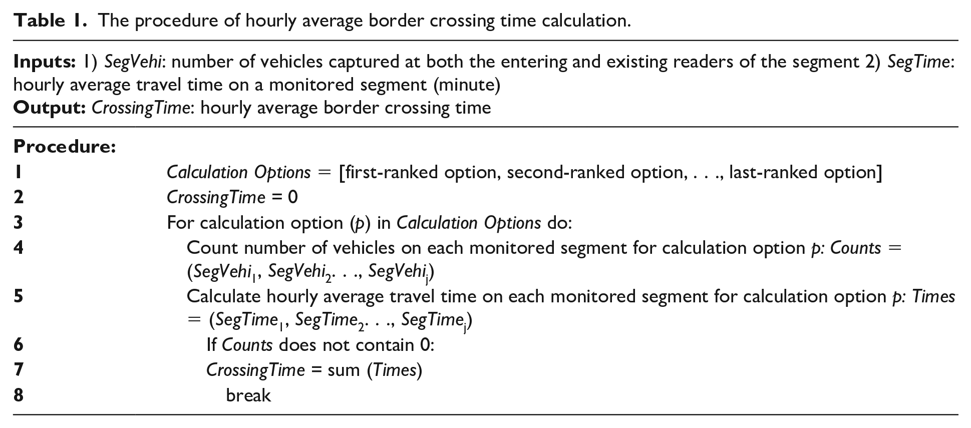
Guided by this procedure, we calculated the hourly average border crossing time using CV data (CV-Time). Since the typical detection range of Bluetooth readers is around 100 meters (Honeywell, 2020), we first created 100-meter buffers around each Bluetooth reader location to extract the CV samples within each buffer, as illustrated in Figure 1. Since the CV data were collected from each trip with a high-frequency sampling rate, multiple waypoints could be captured from the same trip within each buffer. To eliminate the data redundancy, we grouped the CV waypoints within each buffer based on their Journey ID—the unique identifier for every single trip. Then we kept the earliest waypoint for each trip within the first four buffers (Reader 1 through Reader 4) and kept the latest waypoint for each trip within the last buffer (Reader 5). After obtaining the unique trip IDs captured in each buffer, we applied the same procedure as illustrated in Table 1 to calculate the hourly average travel times based on the CV data.
Border crossing time modelling and additional CV-based variables generation
As previously mentioned, the installation and maintenance of the BCIS can be costly. Therefore, there is a practical necessity to investigate whether accurate border crossing times estimates can be made using CV data. In this study, we developed various regression models to estimate border crossing times based on the CV data. We used the hourly averaged border crossing times retrieved from the BCIS as the response variable and the CV-Time and additional CV-based features as predictor variables. A detailed description of the response and predictor variables can be found in Table 2.
Description of the response and predictor variables.
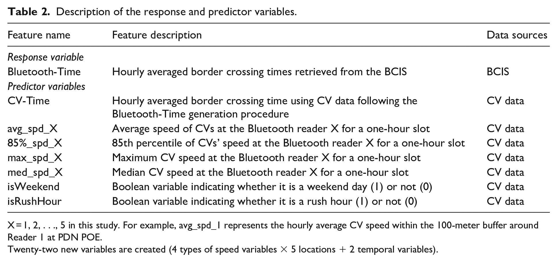
X = 1, 2, . . ., 5 in this study. For example, avg_spd_1 represents the hourly average CV speed within the 100-meter buffer around Reader 1 at PDN POE.
Twenty-two new variables are created (4 types of speed variables × 5 locations + 2 temporal variables).
Studies have shown that traffic congestion patterns vary over time, with different levels of congestion observed during rush hours or on weekends (Dadashova et al., 2021). Furthermore, traffic congestion directly affects vehicle speeds, resulting in spatially varied speed profiles in congested and free-flowing conditions (Huang et al., 2018). Therefore, hourly aggregated CV driving speeds at various locations (Bluetooth readers) could be important variables in modelling traffic congestion. In this study, we developed 20 additional CV-based variables to capture the driving speed dynamics at different locations along the PDN POE, aggregated on an hourly basis. These variables are designed to enhance the accuracy and effectiveness of our model. To obtain the data, we created five 100-meter buffers around each reader to extract CV data. For each location, there were four speed-relevant variables: mean, median, 85 percentile and maximum value of hourly aggregated speed observations. Thus, a total of 20 speed-relevant variables were generated (4 speed-relevant variables × 5 locations [CV extraction buffers]). We also created two temporal variables to differentiate between CV data collected during rush hours (7 am to 9 am and 4 pm to 7 pm) and on weekends.
OLS is a commonly used model to describe linear relationships between one or more predictor variables and a response variable. RF is a supervised learning algorithm that combines the results of a series of decision trees to build a more robust regression model than a single tree. GB is another supervised learning algorithm that builds a predictive model by assembling weak models, such as decision trees. GB builds trees sequentially, with each tree built to correct errors made by the previous tree, making it efficient in handling complex non-linear relationships.
To improve the modelling performance, we also used the feature importance score generated by RF to remove redundant and irrelevant variables. This feature selection approach helped to ensure that only the most relevant variables were included in the final model.
Comparison and evaluation
This study employed two performance metrics, Root Means Square Error (RMSE) and Mean Absolute Percentage Error (MAPE), to evaluate the performance of the models. RMSE and MAPE are widely used measures to evaluate the accuracy of predictions against the actual values. Equations 2–3 illustrate how to calculate these metrics based on two data groups with the same sample size:
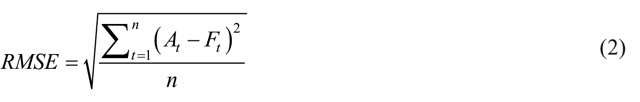
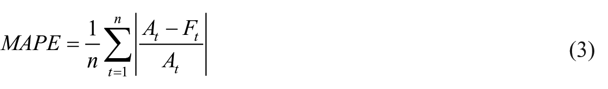
where A represents the actual sample group; and
Result
This pilot study was conducted over a two-month period (September and October 2022) using data from the BCIS and CV data at the PDN POE. A total of 21,196 border crossing trips were recorded, resulting in the accumulation of 1,530,915 waypoints. As the study focused on border-crossing traffic, only a limited number of vehicles were permitted to share their border-crossing traffics, resulting in missing data in certain time slots and diminishing the reliability of direct estimates for border crossing times based on the CV data. To address this, we divided each month into 720 one-hour slots (24 hours/day × 30 days/month) and calculated the CV-Time for each slot, following the procedure introduced in Section 4.2. We marked each slot as either a CV-covered slot or a CV-uncovered slot based on whether or not CV-Time could be generated. In total, we identified 1,057 CV-covered slots, including 512 in September and 547 in October 2022, which were used in our models.
In this study, we conducted several regression analyses to estimate border crossing times based on CV-Time and additional CV-based variables. First, we built a basic OLS model with CV-Time as the sole predictor variable to assess its relationship with ground truth observations. Next, we incorporated different spatially varied speed and temporal variables to enhance the modelling performance. We used 70% of the CV-covered slots (740) as the training dataset to calibrate the models, and tested the models on the remaining 30% of data (317). Two measures, including RMSE and MAPE, were used to assess the performance of the models.
OLS models with CV-Time only
We first built an OLS linear regression model (Simple OLS) using the CV-Time alone as the predicting variable with the ground truth observations (Bluetooth-Time). Figure 4 displays the bivariate scatter plot with a fitted regression line. Alongside the scatter plot, marginal histograms are presented to show the distribution of Bluetooth-Time and CV-Time. Additionally, the figure shows the correlation coefficient plus the significance level, positioned above the fitted line. The symbol *** represents the significance level with a p-value less than 0.001.
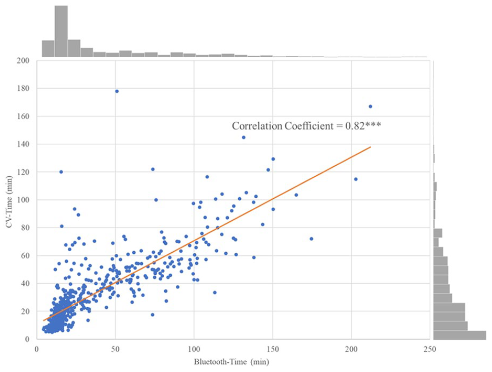
The distribution and correlation plot between the Bluetooth-Time and the CV-Time in the training dataset.
The Bluetooth-Time and the CV-Time are significantly correlated with a high correlation coefficient (0.82) and follow a linear relationship. Therefore, we built an OLS model to represent the linear relationship between the Bluetooth-Time and the CV-Time (Simple OLS). The modelling result and the fitted functional form are detailed in Table 3. The result indicates that the CV-Time is a significant predictor for estimating the Bluetooth-Time. With the CV-Time as the sole predicting factor, 67 percent of the variance in the Bluetooth-Time can be explained by the fitted linear model.
Simple OLS result based on training dataset.
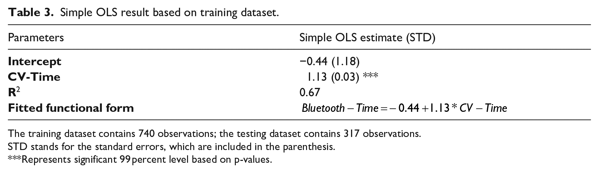
The training dataset contains 740 observations; the testing dataset contains 317 observations.
STD stands for the standard errors, which are included in the parenthesis.
Represents significant 99 percent level based on p-values.
Improved OLS model with additional CV-generated variables
Besides the CV-Time, we also explored whether or not speed-relevant variables and temporal variables can capture spatiotemporal dynamics of congestion patterns so as to enhance modelling performance. Twenty-two additional variables to capture the traffic driving speed dynamics at different locations along the PDN POE aggregated on an hourly basis.
It should be noted that some variables may not be significantly correlated with the response variable, and multicollinearity issues also exist among them. Including irrelevant or interrelated variables in the model potentially may leads to biased estimations. Therefore, we performed RF feature selection to select the optimal subset of predictor variables. RF feature selection is one of the most used feature selection methods, which computes an importance score for each feature by measuring the decrease in impurity resulting from splitting on that feature. We performed RF feature selection on the training dataset, and the results (Figure 5) indicated that 85th percentile of CVs’ speed at Reader 3 (85%_spd_3) is the most important feature, followed by CV-Time, average speed of CVs at Reader 2 (avg_spd_2), average speed of CVs at Reader 3 (avg_spd_3), and 85th percentile of CVs’ speed at Reader 4 (85%_spd_4). Based on the selected variables, we built an improved OLS model (Improved OLS) along with RF and GB regression models for estimating border crossing times.
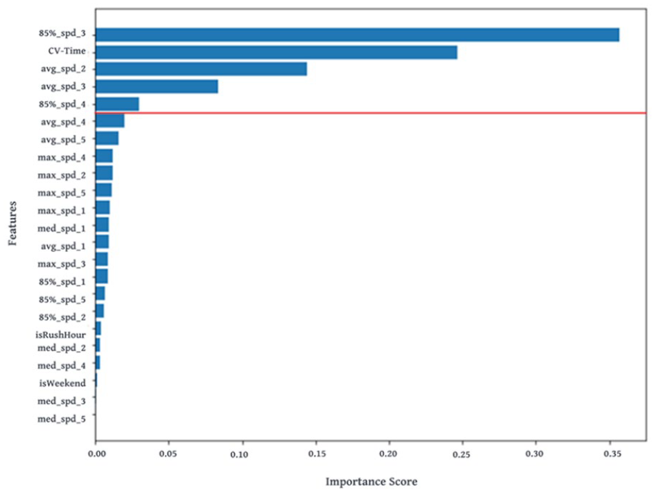
Feature importance scores obtained from RF feature selection.
The modelling results based on the testing dataset are detailed in Table 4. Without modelling, the RMSE and MAPE between directly calculated CV-Times and Bluetooth-Times in the testing dataset are 21.67 and 42%, respectively. By fitting a simple OLS model with the CV-Time as the only predicting variable (Simple OLS), the estimate accuracy can be improved with the RMSE decreased to 18.90. By incorporating the additional variables into the models, all three models (improved OLS, RF, and GB) achieved a better result than the Simple OLS with lower RMSE and MAPE. The GB performs the best among the introduced models, achieving the lowest RMSE of 15.50 and MAPE of 25%. These results suggest that incorporating additional CV-generated variables could improve the performance of the model under conditions of limited data.
Modelling results comparison based on the testing dataset.
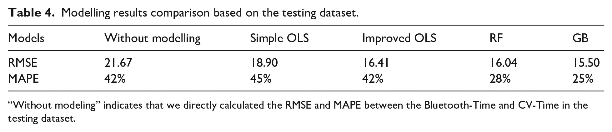
“Without modeling” indicates that we directly calculated the RMSE and MAPE between the Bluetooth-Time and CV-Time in the testing dataset.
Discussion and conclusions
POEs serve as vital gateways for international trade, playing an important role in the US economy. Monitoring border crossing times accurately and effectively is crucial for border transport management. This study marks a pioneering attempt to evaluate the effectiveness of market-available CV data in border congestion studies. Using CV-generated variables, we developed different regression models to estimate border crossing times at the PDN POE in El Paso, Texas, based on CV-generated variables.
Key findings and implications
Our findings suggest that despite having limited samples, market-available CV data can generate highly similar results for border crossing times retrieved from the BCIS, with a correlation coefficient of around 0.82. A GB model fitted based on the combination of CV-Time and additional CV-generated variables outperformed other models (Simple OLS, Improved OLS, and RF) in estimating border crossing times, with an RMSE of 15.50 and MAPE of 25%. Based on the results of our study, market-available CV data holds promise as a data source for monitoring border crossing times. We recommend that market-available CV data could be used to supplement the existing BCIS and serve as an alternative solution when the BCIS is down for maintenance.
Although this study was based on a limited sample of two months of CV data, the accurate modelling results indicate the possibility of replacing the existing Bluetooth-based system with the CV data if we could obtain sufficient CV samples at all hours every day. Although this study focused on border-crossing traffic, our findings suggest that CV data could also be valuable in for investigating other types of congestion problems (e.g., most congested road identification, traffic congestion assessment) beyond border congestion issues. With the maturing of the CV data market, we encourage researchers to leverage multi-source CV data in their studies to improve the data coverage and advance transportation research.
Challenges associated with CV data application
As previously mentioned, this study only obtained 1,057 CV-covered slots, which accounts for approximately 73.4% (1,057/1,440) of the total one-hour slots. The remaining 26.6% of one-hour slots were not examined due to missing data. Note that two possible reasons may exist, leading to the limited coverage of the CV data in the PDN POE. First, the 2022 CV data provided by our data supplier can only share border-crossing traffic data collected from one of its partnered original equipment manufacturers (OEMs), which significantly limits the available sample sizes. Second, this study has a specific data requirement for CV data with a specific interest on border-crossing trips from Mexico to the US, but due to data sharing restrictions, only data from US-registered vehicles can be collected, resulting in a lack of data for Mexico-registered vehicles.
It is worth noting that while new technologies like CVs have undoubtedly brought many benefits to society, such as enabling smart services, they can also contribute to creating inequalities, specifically the digital divide (Shin et al., 2021). Least-developed and developing countries often have limited access to these technologies. To the best of our knowledge, current market-available CV data is only collected from certain developed counties, such as the US and some European countries, which creates a form of technological inequality. In addition, the adoption of fine-grained driving data raises a lot of political, legal, and ethical concerns. Different countries or governmental agencies have launched different laws and regulations to regulate the collection and use of the individual-level data, resulting in heterogeneous data formats and contents across counties (Li et al., 2021). This significantly hampers the use of fine-grained data for solving international issues. To promote the adoption of this emerging data in future transportation management, efforts need to be made not only to improve data availability for developing countries but, more importantly, to standardize guidelines for data collection and utilization through joint efforts from both public and private sectors.
Limitations and future work
This study can be improved from three perspectives: improve the experimental settings, advance the estimation models, and extend the evaluation period. First, due to data licensing limitations and the lack of ground truth observations, we only examined two months of CV data at one POE—the PDN POE with travel time estimates generated at one-hour interval. This evaluation was conducted based on the 2022 CV data, whose border crossing data are only from one OEM with a relatively low penetration rate, resulting in limited CV samples. Therefore, the performance of using CV data in border crossing time estimation at other POEs, especially with different temporal scales, may differ. For further determining how to incorporate the CV data into the current border-monitoring system, there is a practical necessity to evaluate the latest CV data obtained from different CV data providers to see if a broader coverage and higher penetration rate of CVs at different POEs over a more extended study period can be achieved.
Second, to ensure the feasibility and simplicity of implementation, our study primarily employed straightforward modelling approaches, including OLS, RF, and GB. However, we acknowledge that numerous advanced models, particularly those based on graph theories (Salamanis et al., 2016) and deep learning (Zhang et al., 2018), have shown promising results in travel time prediction with diverse data sources. These advanced methods could be considered for integration into our study as the penetration rate of CVs at POEs increases, potentially leading to improved model performance. Last, this study was conducted based on historical CV data, limiting its application to real-world settings. Future efforts can be made to focus on assessing and using streaming CV data to move toward a real-time solution monitoring border crossing times at border crossings.
Footnotes
Acknowledgements
The authors also acknowledge the contributions made by Swapnil Samant, David Salgado, and Rafael Aldrete.
Declaration of conflicting interests
The author(s) declared no potential conflicts of interest with respect to the research, authorship, and/or publication of this article.
Funding
The author(s) disclosed receipt of the following financial support for the research, authorship, and/or publication of this article: This work was supported by the Center for International Intelligent Transport Research, Texas A&M Transportation Institute under Grant [185921-00011].