
Abstract
There is a rich literature connecting for profit financial portfolio theory to non-profit organisations’ funding diversification policies. This research typically ignores fundamental specificities of the non-profit context. The present paper integrates three of these specificities: non-profits’ performance being measured by other standards than their financial profitability, the non-proportionality between funding expenses and expected incoming funds due to varying marginal effects of the former, and crowding in/out effects between non-profit funding sources. It is shown that, contrary to what is the case in financial portfolio theory, a positive relation between expected performance and its variability cannot be taken for granted when increasing the number of non-profit’s funding sources. An important reason for this is the presence of crowding effects, which therefore cannot be ignored when looking for the best non-profit’s funding diversification strategy.
Introduction
Non-profit organisations are commonly defined as organisations founded to pursue non-financial objectives, not allowing the distribution of any financial surplus to owners or staff (Hansmann, 1987). Having other objectives than wealth maximising implies that their managerial behaviour (in all functional domains) can differ from that of the for profit organisations. Obviously, like all other kinds of organisations, they need financial resources to enable their operations. Those resources can be drawn from different sources, such as donors, governments, clients, and endowments, none of them necessitating the pursuit of financial returns, unlike the financial sources feeding for profit organisations.
It is generally accepted that non-profit organisations have more potential financial sources than for profit organisations (Tuckman, 1993). Their observed combination henceforward will be called the organisation’s funding portfolio. Young’s (2017, 41, 45) ‘benefits theory’ posits that the composition of this portfolio depends on the organisational mission and the ensuing activities and perceived benefits. This insight is consistent with the observation by Chang and Tuckman (1994, pp. 281–284) that industry affiliation, reflecting a specific category of missions, affects non-profit funding portfolio diversification (capturing both the number and distribution of financial resources in the funding portfolio). A link with institutions (and hence with institutional theory) is already found in results by Salamon and Anheier (1998, p. 219), who document marked differences in funding portfolio composition between countries (controling for industry).
Starting with Chang and Tuckman (1994), there is a long tradition of empirical research linking funding diversification to non-profit organisations’ financial health/vulnerability, 1 mostly presented in a resource dependency framework. This has yielded qualitatively diverging conclusions as to the question whether more or less portfolio diversification is beneficial, balancing dependency considerations relevant in case of a few (or one) source(s) and rising fundraising costs together with possible mission-related conflicts in case of numerous sources.
As to theory on non-profit fundraising diversification, since the publication of Kingma’s (1993) seminal paper applying ‘modern’ financial portfolio theory (Markowitz, 1952) to select a portfolio of non-profit organisations’ funding sources (government and donations in his case), this theory attracted much research attention. Comprehensive literature reviews by Hung and Hager (2019) and Qu (2019) provide excellent and up-to-date states of the art, but also the warning that ‘one must be very cautious in directly transplanting portfolio theory into the nonprofit setting without considering … complications’ (Qu, 2019, p. 210). An obvious reason for this is the fact that non-profit performance differs from purely financial performance. Another problem, already alluded to by Jegers (1997, p. 68), is the observation that traditional portfolio theories discuss the composition of financial portfolios generating independent (albeit correlated) incoming streams of financial revenues (interests, dividends, gains realised when selling financial instruments), whereas the non-profit funding portfolio literature deals with the configuration of periodically incoming funds possibly directly affecting each other such as the abovementioned subsidies/grants and donations, or, among others, programme/earned revenues, all of which can be subdivided in finer-grained categories. Each of these categories is linked to a ‘funding source’, from which funds can be tapped as the consequence of specific expenses (e.g., fundraising expenses), which in cases of spontaneously incoming funds might be zero. In what follows these expenses will be called ‘funding expenses’.
This has at least two important implications, justifying the development of a financial portfolio model focused on non-profits. First, investors in financial portfolios can exactly determine the expected return of each instrument in their portfolio, the expected return being proportional to the amount invested in the instrument, a proportionality which cannot be expected when considering the relation between funding expenses and the amount of incoming funds, as one cannot a priori assume the marginal effect of funding expenses to be constant, each additional Euro of funding expenses not always raising the same amount of funds.
Second, financial portfolio theory does not consider crowding in/out effects known to characterise relations between non-profit organisations’ funding sources. One such effect is the extensively studied interaction between donations and subsidies assessing whether higher levels of one lead to higher or lower levels of the other. 2 Such crowding mechanisms are fundamentally different from random co-movements, called hereafter stochastic correlations, implying that both should be explicitly distinguished, in theory as well as in empirical work.
The present paper presents a dedicated theory of non-profit organisations’ funding diversification accounting for the abovementioned differences between the for profit and non-profit funding contexts. 3 A novel taxonomy of conceivable non-profit organisations’ funding portfolio models is presented combining the absence/presence of crowding effects with the absence/presence of stochastic (co)variations. Original insights, contributing to the extant non-profit funding portfolio theory, are derived from the implications of the different models. Firstly, the traditional positive risk-performance association and the ensuing portfolio selection steered by risk attitudes will not automatically prevail, as ‘traditional’ diversification strategies will not always reduce the non-profit funding portfolio risk. Further, it will be shown that, as a consequence, optimal funding portfolios need not contain funds from all available funding sources, also contrasting with financial portfolio theory, in which by virtue of the separation theorem optimal portfolios are a combination of a risk-free asset and the market portfolio, by definition containing all financial assets.
In what follows the different non-profit funding portfolio models studied will be presented in ascending order of complexity and realism. For each model mathematical optimisation techniques will be used to characterise ‘optimal’ portfolios in terms of organisational performance and performance variability. Practical implications will be suggested. In the concluding section, the model’s main implications will be reiterated, followed by a discussion, an overview of limitations, and opportunities for further research.
Portfolio Models of Funding Diversification in Non-profit Organisations
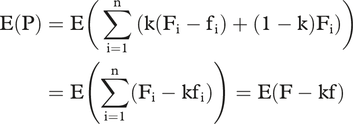
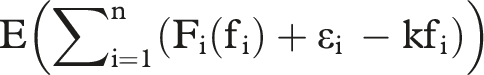
We assume the non-profit organisation has an organisational objective function P, which is not financial profitability as in traditional portfolio theory. It is commonly known that in non-profit organisations, as elsewhere, managerial objectives need not coincide with board objectives (Van Puyvelde et al., 2012). Thus we model P, in line with the seminal work of Steinberg (1986), in a stylised way as the weighted average of service level (reflected by the amount of funds available for providing services) and budget level (gross funding amount). The weight k (∈[0,1]) is determined by the relative power, respectively, of board (assumed to prefer as much activity as possible) and management (assumed to strive for as high budgets as possible), and is therefore an indicator of management-board agency problems within the organisation. When the board (management) has all the power, k = 1 (k = 0). 4 The eventual objective pursued by the organisation (P) is the outcome of a balancing process between board and management.
Considering n funding sources, this leads to the following expression for the expected organisational performance, given the level of funding expenses, E being the expected value operator:
If there is no uncertainty as to the funds generated, striving for the highest attainable performance level (P*) is optimal.
If however the funds generated are stochastic, uncertainty comes into play. Then, optimality will be determined by the interplay among three factors: the expected level of P (called in what follows ‘expected performance’), its variance (‘performance variance’), and the level of organisational risk-aversion or, in other words, the expected performance the organisation is willing to sacrifice for a reduction in performance uncertainty. If risk-neutrality prevails, maximising P will determine the optimal funding portfolio as for the case without uncertainty.
Six different basic models can be considered, differentiated by the (non) inclusion of crowding effects, stochastic effects εi,
6
and correlations between funding sources
7
: No crowding, no stochastic effects: No crowding, stochastic effects: No covariances between funding sources: cov(εi, εj) = 0 for i ≠ j Covariances between funding sources: cov(εi, εj) ≠ 0 for i ≠ j Crowding, no stochastic effects: Crowding, stochastic effects: No covariances between funding sources: cov(εi, εj) = 0 for i ≠ j Covariances between funding sources: cov(εi, εj) ≠ 0 for i ≠ j
Clearly, the more complex models are more realistic.
No Crowding, No Stochastic Effects
As this is a non-random, deterministic, case, no expectation operator is needed to derive the optimal funding portfolio (F1, …, Fn):
For each funding source i the amount invested, assuming interior solutions, should meet
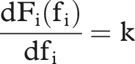
Given the concavity of
No Crowding, Stochastic Effects, No Covariances Between Funding Sources
Introduction
Now, we consider not only the expected value of P, but also its variability,
8
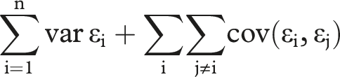
which with no covariances is simply the sum of the variances related to each funding source:

The conditions derived in the previous section also now characterise the maximally attainable level of P (P*), being the effect of optimal funding expenses
Equal Variances
In this case
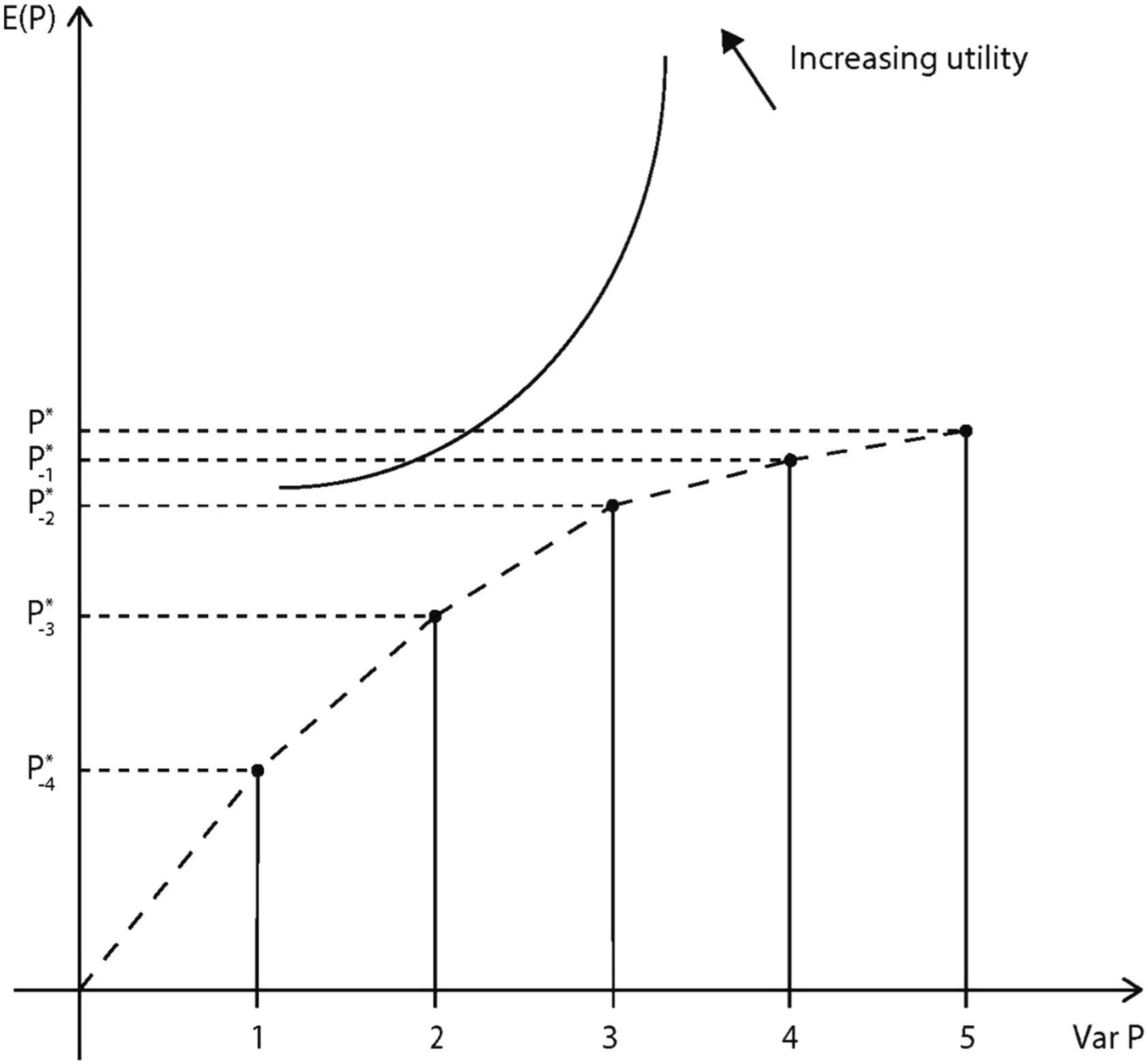
Performance variance-E(P) curve (no crowding, no covariances, constant and equal variances).
Different Variances
In a more general case, we have
No Crowding, Stochastic Effects, Covariances Between Funding Sources
Introduction
Now, expected performance and performance variance are:
Equal Variances and Correlations
We start again with the simplest case: equal variances (

For a portfolio of s (≤n) sources this becomes

Variance by definition being positive implies the following condition for ρ:
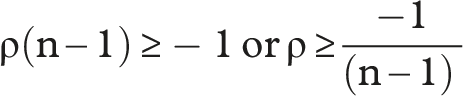
In the limiting case
Going from s sources in the portfolio to (s + 1) sources changes the performance variance independently from the specific funding sources involved by

The conditions for reaching the highest possible E(P) still are the same, as is the observation that performance variance can only be affected by increasing/decreasing the number of funding sources, but not by changing funding expenses.
If
Diversification benefits, in the sense that performance variance is smaller due to correlations between funding sources than without correlations, can only occur for a negative value of
If
The second situation will arise when
The third situation occurs when Example of a performance variance-E(P) curve without crowding and with constant and equal (co)variances.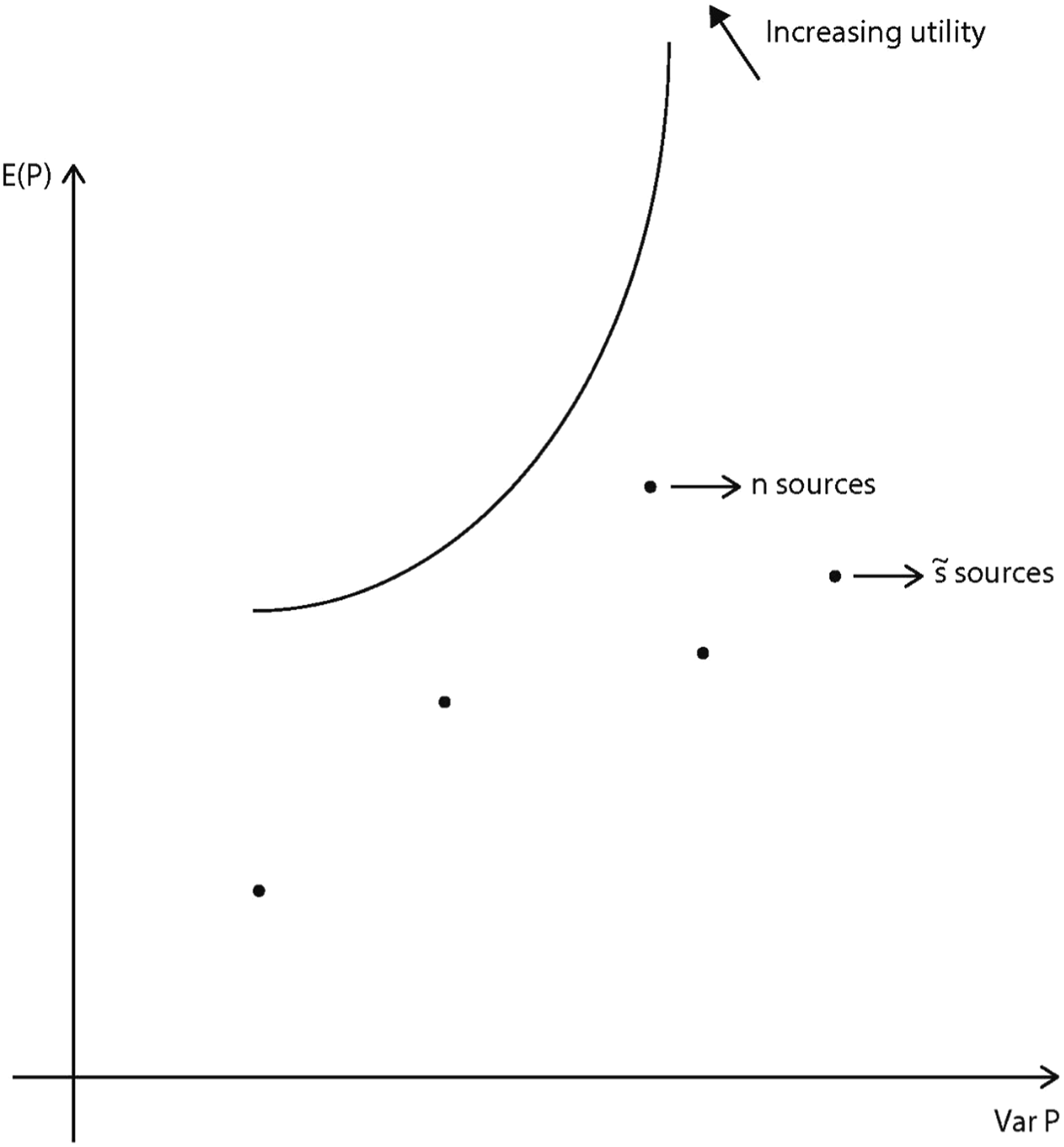
Different Variances and Correlations
As in the section ‘Different Variances’ when analysing the situation without crowding but with stochastic effects and no covariances between funding sources, we now have
A first case is the one in which all covariances are positive. As in that same section, and as shown in Appendix 2, we start from the P* portfolio and sequentially drop from the remaining s funding sources the source i for which
The next case
13
is that when all covariances are negative. Dropping a funding source (i) from a portfolio of s sources results in the following reduction (which can be negative, then reflecting an increase) of the performance variance:
The correlations being negative, three subcases are a priori possible: the reductions (call them, with a common symbol, Δ) are all positive for all s, they are all negative for all s, and some are negative while other are positive. The first subcase (implying the correlations are (very) small in absolute terms) can be analysed in the same way as the case of positive correlations. The second subcase implies that adding a funding source would always both increase E(P) and decrease the ensuing performance variance, automatically making the portfolio combining all sources at their values

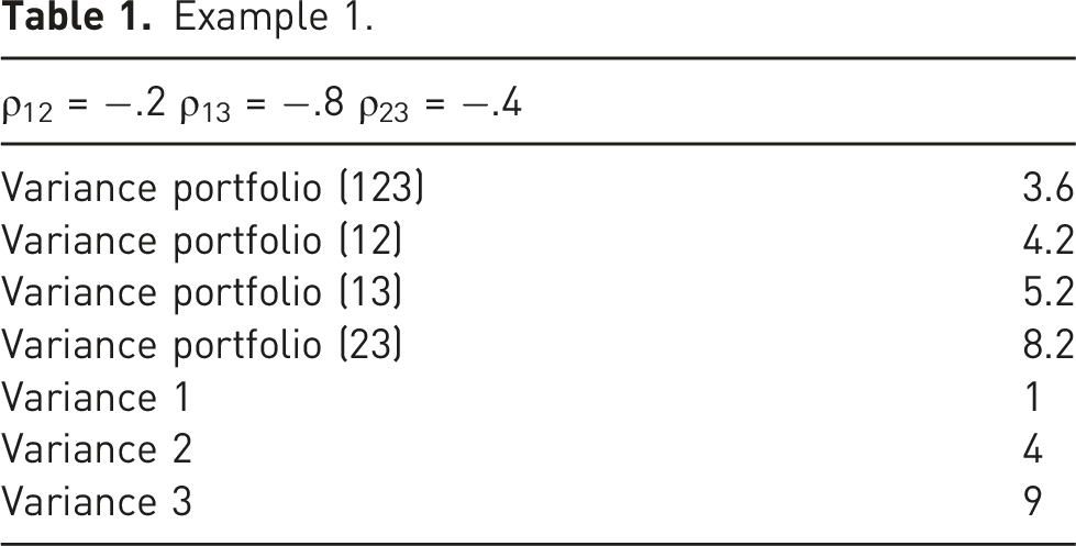
Example 1.
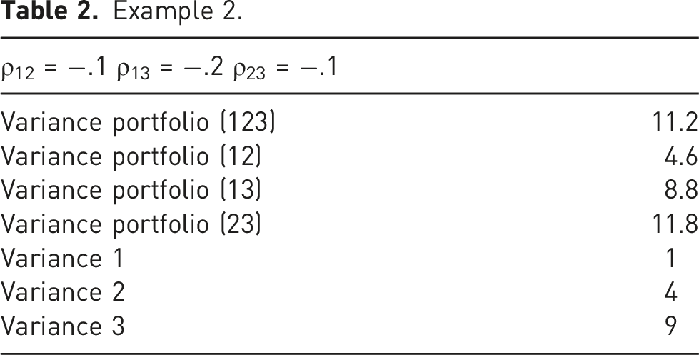
Example 2.
Example 3.

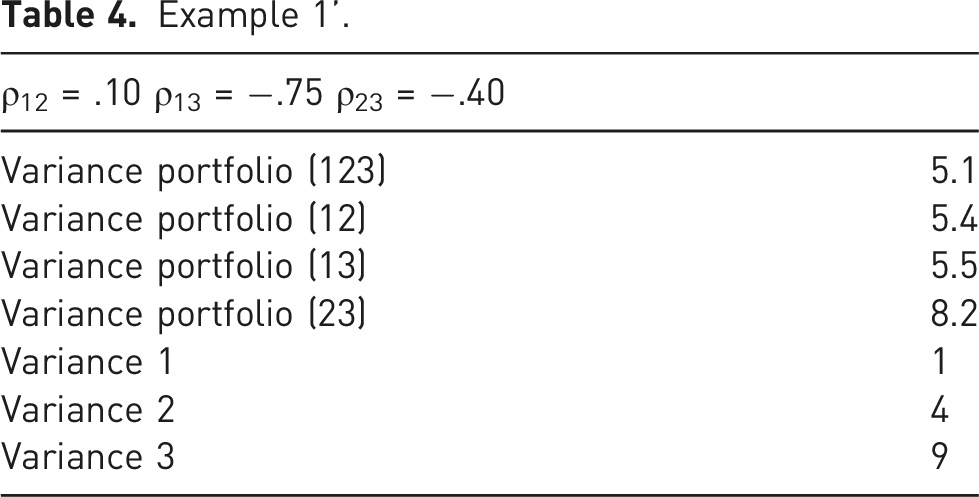
Example 1’.
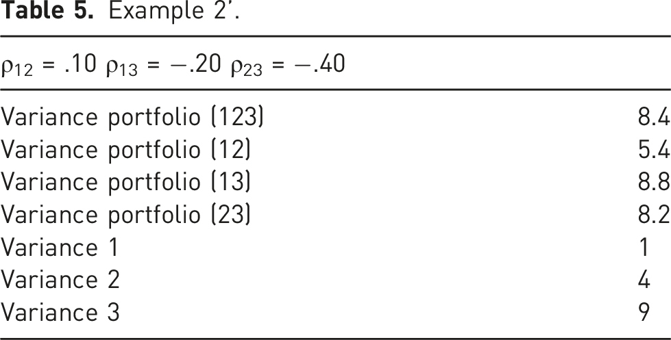
Example 2’.
Example 3’.

Crowding, No Stochastic Effects
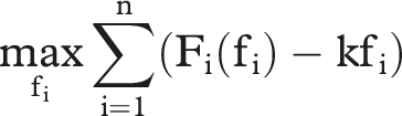
This is basically a simple case, even though its solution might be numerically complex, depending on the articulation of the relationships involved. For given values of fi we indeed have a system of n equations in n variables Fi, which, if it meets the regularity conditions, can be solved. The value of P obtained then is function of the fi, so it can be maximised by solving for the optimal values of the fi.
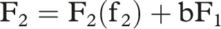
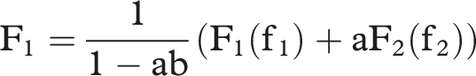
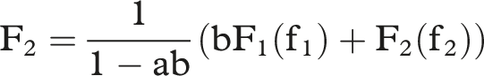
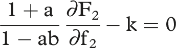
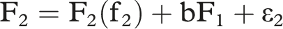
Suppose, in a simple algebraic example, two funding sources (n = 2). The crowding in/out effects are reflected by the parameters a and b in the equations below. Positive (negative) values reflect crowding in (out). To avoid pathological outcomes, we assume the absolute values of a and b to be below 1. In a simple additive model we assume the level of funding Fi equals the funds raised by the funding efforts fi to which the crowding effect of Fj (j ≠ i) is added: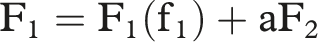
Acknowledging the absence of stochastic variability, the ensuing value of P then is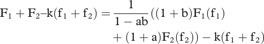
If there is an interior maximum, the concavity of Fi(fi) guarantees its uniqueness when the following conditions are met: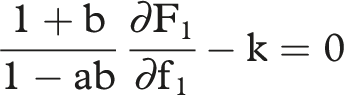
Crowding and Stochastic Effects
The model discussed in the section ‘No Crowding, Stochastic Effects, Covariances Between Funding Sources’, is a special case of the more general model in which crowding, stochastic effects, and covariances between funding sources are considered. It was established that even in this special case one cannot be sure the curve linking the relevant performance variance-E(P) pairs is concave. Hence, this also applies to the case with crowding effects and non-zero correlations.
The model with crowding effects, but no correlations between funding sources, generalises the model described in the section ‘No Crowding, Stochastic Effects, No Covariances Between Funding Sources’, where it was established that the curve linking the relevant performance variance-E(P) combinations was concave. We now show that this can not longer be guaranteed any more. To that end, we generalise the algebraic example of the previous section: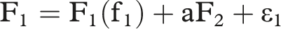
The maximum E(P) is the same as described in Section 2.4, but now comes with performance variance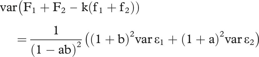
In the simplest case where variances of both funding sources are equal this becomes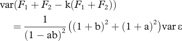
Performance variance reduction by eliminating one of both funding sources has the sign of
Considering the even more special case in which a = b this becomes
Practical Implications
Despite the present paper being theoretical in nature, there are practical implications, especially from the more realistic models. The first is that it need not be true that increasing the number of funding sources automatically leads to ‘better’ portfolios. The second is that the traditional (financial) diversification logic is not always valid regarding performance variability, necessitating consideration of crowding effects among potential financing sources. Executives (or consultants) of non-profit organisations obviously cannot be expected to engage in calculations implied by this paper, but they might benefit from at least considering intuitively the underlying mechanisms.
Conclusions, Implications, Limitations, and Suggestions for Further Research
Apart from suggesting the abovementioned practical implications, this paper adds to non-profit funding portfolio theory by combining elements of financial portfolio theory and the idiosyncrasies of non-profit organisations’ funding streams, leading to theoretical results not always similar to the ones obtained in classical portfolio theory or the extant non-profit funding diversification literature. Fundamental characteristics, including the performance indicator and the role of crowding in/out effects, markedly differ between for profit and non-profit funding contexts. These elements are now for the first time integrated in a more comprehensive theoretical approach to non-profit funding portfolios. The main insight obtained is that, contrary to financial portfolio theory, general statements about optimal funding portfolios of non-profit organisations cannot be made, which might explain the ‘diverging conclusions’ of the empircal literature referred to in the Introduction. The composition of optimal non-profit funding portfolios is shown to be determined by the severity of agency problems between board and management, the specific values of performance variances and covariances and the crowding structure linking the available funding sources. Crowding effects indeed can even invert diversification effects resulting from stochastic relations between funding streams: in these cases, portfolio risk might increase by adding funding from additional sources, instead of being reduced.
Models like the ones elaborated in the present paper are characterised by limitations and omissions, which in turn might inspire further extensions and refinements. A number of them are enumerated above (organisation level, (sub)sector level, and ecosystem-related effects on expected funding streams, specific non-profit regulations as to fundraising, dynamic mechanisms including potential ‘starvation cycle’ effects (Schubert & Boenigk, 2019) 14 ). Further, apart from amending the traditional Steinberg (1986) approach of reflecting the organisational objective in monetary units and only considering activity level (board) and budget (management) determining the eventual organisational objectives (ignoring other potential stakeholders such as the funders themselves: large donors, governments, …), 15 the implications of more articulated specifications of the stochastic and crowding effects might be established. Finally, the models developed in the present paper make abstraction of the institutional context. Their potential usefulness could be enhanced by taking this context in consideration, theoretically or (in particular) empirically by ‘incorporat[ing] various institutional contexts to test the model’s applicability’. 16 Examples of elements that might be considered are fiscal rules on donations and non-profit surplus, and subsidy regulations, 17 to which more general constructs at the jurisdictional level might be added.
Also concerning empirical research, the reviews referred to above show that the distinct literature streams on non-profit funding portfolios and crowding effects are isolated from one another: empirical non-profit funding portfolio work ignores crowding effects, and the empirical crowding literature abstracts from any funding portfolio consideration. The results obtained in the present paper imply that both should be integrated.
Footnotes
Author Notes
The constructive comments of the anonymous referees and the editor-in-chief Rotem Schneor are gratefully acknowledged. Sofie Devos and Joshua Holm respectively provided excellent technical and editorial support.
Declaration of Conflicting Interests
The author declared no potential conflicts of interest with respect to the research, authorship, and/or publication of this article.
Funding
The author(s) received no financial support for the research, authorship, and/or publication of this article.
Notes
Appendix 1
To fix ideas, consider the case of a non-profit organisation having access to three funding sources. Call them 1, 2, and 3 which, e.g., could signify donations, grants, and unrelated business income. Expenses to generate funds of each category are respectively f1, f2, and f3, whereas the funds raised in each category are F1, F2, and F3.
In the simplest model (no crowding, no stochastic effects) there is, for each funding source, a deterministic relationship between funding expenses and funds raised. The simplest relationship is linear (with all coefficients being positive):
Assuming such a relation does exist is equivalent to assuming some level of covariation between the stochastic differences, e.g., induced by some common randomly occurring external factors impacting on the levels of funds raised. These impacts need not be the same for all sources. To give just an example: the impact of a financial crisis might be more substantial for donations than for grants, even though they might go in the same direction.
The third model describes a deterministic case with crowding effects, which means that the funding obtained from one source affects (positively (‘crowding in’) or negatively (‘crowding out’)) the level of funds obtained from another source. A simple way to describe this analytically is as follows:
The last models again add stochastic differences to these expressions, without and with covariations respectively.
Appendix 2
In order to prove the concavity of the kinked curve connecting the s performance variance-E(P) points constructed according to the ascending rule, we proceed as follows.
Suppose this rule makes us drop funding source i’ first, and then i”. The other (s-2) sources then remain in the portfolio after these two eliminations. The fact that i’ is chosen first means that
As all covariances are positive, the RHS of this inequality is smaller than