
Abstract
Savings Groups (SGs) are informal community-based entities that act as grassroots financial cooperatives. They provide financial services to their members over an agreed-upon time period, commonly referred to as a ‘cycle’. During this cycle, saving and borrowing transactions take place during regular member meetings. Using new data on SGs worldwide, we conceptualize and quantify SG performance at the group level. Starting from the financial economics of the SG model, we introduce the savings capacity, profit-generating capacity, and borrowing conditions as complementary performance dimensions. We study these dimensions both across and within cycles to capture the financial efficiency of SGs. Our findings suggest that while SGs strengthen savings capacity over time, they primarily act as short-term cash-management vehicles. Groups prefer easy and affordable loans for emergencies over profit generation via micro-lending. The profit-generating capacity is curtailed by two major implementation restrictions, namely, loan-tying and unproductive periods at the beginning and end of the cycle. Based on our statistics, we formulate recommendations related to the cycle setup and lending policies.
Keywords
Introduction
Despite efforts to improve financial inclusion, rural poverty continues to persist (Robert et al., 2021). Even with substantial microfinance growth, it appears that the poorest households are still not sufficiently reached (Ksoll et al., 2016). In this context, the importance of savings as a crucial component for poverty alleviation has gained traction. While precautionary savings allow to cope with idiosyncratic shocks, the accumulation of a financial buffer allows to manage liquidity constraints and smooth household consumption (Karlan et al., 2014).
Savings groups (SGs) are informal financial institutions with a longstanding history that are increasingly explored as a tool for financial inclusion. Even with the rapid expansion of modern banking technologies, these informal group-based models continue to exist alongside formal financial services (Redford & Verhoef, 2022). More than 100 million people currently entrust their savings to this informal financial system (Burlando & Canidio, 2017; Greaney et al., 2016). Many development actors have now started to actively promote SGs to stimulate financial access and bring development services to poor communities worldwide. Understanding whether SGs succeed in catering to the financial needs of their members and stimulate financial inclusion is therefore of vital importance.
Academic research on the SG phenomenon has mainly focused on how these groups operate and what benefits they bring to members. One strand of literature, for example, studies the economics of SGs as well as their contextual logic (Biggart, 2001; Bouman, 1995; Handa & Kirton, 1999). Several authors have focused on member benefits, notably the insurance mechanism, risk diversification mechanism, or savings mechanism inherent in group participation (Ambec & Treich, 2007; Calomiris & Rajaraman, 1998; Klonner, 2003). Other studies focus on member outcomes in terms of asset accumulation, welfare enhancement, or related outcome parameters (Beaman et al., 2014; Karlan et al., 2017).
Because of the emphasis on individual member outcomes and motivations, less is known about what constitutes financial performance at the group level. It is not clear whether SGs are financially efficient, i.e., enable financial welfare creation for their members. This paper aims to address this gap by treating SGs as microeconomic entities and studying group-level financial performance. This offers valuable insights both to academics and to practitioners currently promoting SGs. While we realize that financial outcomes and associated indicators do not fully recognize the social dimension of the SG model, evaluating financial performance is key in assessing the financial sustainability of the SG banking model. Mapping what constitutes group-level financial performance may also allow us to detect potential implementation restrictions inherent to the model. It is also important for donors who want to encourage the promotion of a sustainable implementation model in support of financial inclusion.
We explore a novel database, namely, the SAVIX funded by the Bill and Melinda Gates Foundation. The SAVIX collects standardized group-level financial data at the global level thus allowing us to construct performance variables that were previously unobservable at the group level. Hence, this encompassing dataset allows us to track the financial performance of SGs worldwide. Starting from the financial economics of the SG model, we discuss what constitutes financial performance and present summary statistics on different performance dimensions. We define three complementary performance dimensions that stem directly from the SG operational model: savings capacity, profit-generating capacity, and borrowing conditions.
An important novelty in this paper is that we report both across- and within-cycle statistics on SG performance variables. Given the time-bound nature of the SG model, i.e., a yearly cycle in which operations take place, this offers an important added value. Within-cycle statistics give us insights into savings and borrowing dynamics throughout the yearly cycle. Across-cycle statistics allow us to assess the financial potential of the groups across consecutive cycles. Overall, our statistics suggest that SGs are predominantly used as cash-management vehicles to balance out asymmetric income and unexpected expenses, i.e., emergency lending. The profit-generating capacity is curtailed by implementation restrictions that impede the potential of members to leverage long-term profitable investments via SGs.
The paper is structured as follows. The next part introduces the financial economics of the SG model, previous research findings, and the justification for our financial performance dimensions. Next, we introduce the SAVIX database in more detail and sketch the performance variables used to analyze the performance dimensions introduced in the previous part. Afterwards, we present global statistics on the different performance dimensions under study. Finally, we conclude and present the implications of our findings.
SG Financial Economics
SGs and Related Literature
Savings groups (SGs) have a long tradition in developing countries. They can be understood as informal community-driven ‘collective action’ institutions which pool community resources from a group of socially connected people such as family, friends, community members etc. (Redford & Verhoef, 2022). Some well-known examples of indigenous SGs include ROSCAs (Rotating Savings and Credit Associations) and ASCAs (Accumulated Savings and Credit Associations) studied for instance in Bouman (1995). However, given the strong diversity among SGs, they can go by many different names and organizational principles often linked to their cultural and historical embeddedness.
A specific type of SGs that discerns itself from these indigenous models is the facilitated SG model, i.e. initiated by an external party. The facilitated SG model was first introduced by Care International in Niger in 1990 (called ‘Village Savings and Loan Association’ or VSLA). While similar to ASCAs, VSLAs are mobilized by a facilitating agency and receive training on how to manage their operations (Allan & Panetta, 2010). 1 Following the introduction of the VSLA model, SGs became a widely promoted group-banking model among development agencies. Through the facilitation of SGs, either directly or through a local NGO, development agencies aim to ensure the accommodation of financial services and to foster financial inclusion.
While growing interest in SGs has resulted in many adaptations of the original VSLA model, the basic properties of the facilitated model remain largely unchanged. A first feature is that they are well-embedded in local, mostly rural, communities and are formed, owned, and managed by the members. Groups typically consist of approximately 20 self-selected members that conduct financial transactions among themselves. Democratic governance is an essential pillar of SGs. Hence, they act as small-scale, grassroots financial cooperatives (Allan & Panetta, 2010). Groups operate over an agreed-upon cycle, typically one year. Throughout the cycle, collective savings are mobilized through sequential, often weekly, contributions by all members (Burlando & Canidio, 2017).
Accumulated group savings are stored in a cashbox and allow for the issuance of short-term micro-loans (Burlando & Canidio, 2017). The interest is set by the group ex ante and typically ranges from 5% to 10% per month (Allan & Panetta, 2010). Loan duration is three months in general and borrowers are subject to important borrowing constraints. All members need to agree on the purpose of the loan and members can only borrow three times as much as the amount saved at the time of the loan (Burlando & Canidio, 2017). This ‘loan-tying’ implies that to receive a loan, individuals must first contribute savings to the group. Besides the provision of loanable funds, members often decide to also contribute small amounts to a ‘social fund’ used for emergencies (Brannen & Sheehan-Conner, 2016; Coleman, 1999; Ksoll et al., 2016). At the end of the cycle, both accumulated savings and accrued interest on loans are redistributed among members in what is called the share-out. During this yearly event, all profits made throughout the cycle are shared among members in proportion to their inputted savings.
The ability to mobilize savings that can be converted into interest-bearing loans is the core business of SG operations. Therefore, saving efforts and repayment discipline by SG members is crucial to ensure survival of the group. Morduch and Armendariz (2010) argue that loan repayment is higher when there are high (social) opportunity costs of default. Self-discipline in terms of savings and loan repayment prevents members from being excluded from future cycles (Anderson et al., 2009). Therefore, the repayment discipline in SGs is generally very high. This is confirmed by a limited value of loans write-off, since only .8% of the groups have written of loans (Mersland, 2019).
In the literature, motivations for joining SGs have received much attention. A number of studies focus on the financial benefits, notably access to previously unattainable savings, lending, and insurance instruments (Besley et al., 1993; Lemay-boucher, 2012; Steinert et al., 2018). The group funds, accessible at any time in the form of micro-loans, allow members to balance out asymmetric income and spending patterns. Hence, they allow households to manage idiosyncratic risks and cash-flow shocks (Aker et al., 2020; Pitt et al., 2002). Similarly, additional risk-insurance mechanisms are ensured by the social fund which offers interest-free loans to members in case of an emergency (Allan & Panetta, 2010).
In addition to financial benefits, a number of studies emphasize the socioeconomic benefits of participating in SGs. A large body of literature refers to the ‘social capital’ of SGs, built through social interactions like the weekly group meetings (Knowles et al., 2013; Roodman, 2011). Gugerty (2007) notes that since individual savings are made illiquid when brought into the group, they are protected from being claimed by relatives, stolen, or lost. Anderson and Baland (2002) report that women join groups to protect their savings from their husbands. Intra-household conflict and differences in bargaining power are also cited as reasons to join (Kedir & Ibrahim, 2011). Others have studied SG participation as a self-commitment mechanism. Since illiquid savings cannot be easily withdrawn, SGs encourage more prudent and long-term financial management (Gugerty, 2007; Kast et al., 2018). Hence, different intrinsic motivations may underlie SG formation, which contributes to their substantial diversity and complexity.
There are however also studies that warn against potential social downsides to organizing financial services in group models. In particular, it can lead to social exclusion and social costs arising from peer pressure and monitoring (Anggraeni, 2009; Gugerty, 2007; Wydick, 1999). For example, it is well-documented that disabled persons are typically excluded from group-based financial services (Beisland & Mersland, 2014). Some studies also find evidence of ‘elite capture’ where group leaders extract most of the rents at the expense of other members (Guha & Gupta, 2005).
An interesting discussion relates to the question of whether development actors should promote SGs. Bouman (1995) warned long ago against too much involvement from the development community because of the risk of ruining a well-functioning indigenous financial system. Similarly, it has been argued that the interest rate applied in facilitated SGs conflicts with their reciprocity-based logic (le Polain et al., 2018). Yet, other studies have suggested the valuable role development agencies can play, e.g., by stimulating transparency, providing additional development services, and ensuring inclusion of the most vulnerable people within the community (Guha & Gupta, 2005; Mersland & Eggen, 2007; Roodman, 2011).
Despite growing interest, there is some debate regarding the potential of SGs to transform the lives of the poor. So far, comprehensive impact studies show mixed results on financial inclusion and poverty reduction (Beaman et al., 2014; Karlan et al., 2017). Similarly, Burlando et al. (2021) show that SGs may be unable to accommodate the needs of their members due to potential mismatch between supply and demand for funds. An excess of funds is associated with lower returns on savings, whereas fund scarcity results in loan rationing (Burlando et al., 2021). Although this scarcity results in high returns on savings (since funds are not left in the cash-box unused) it also discourages members to save since their leverage potential is limited. Overall, the authors show how the resource constraint in the group, i.e. the money available for lending in the cash-box, poses a binding constraint which causes individual decisions on saving and borrowing to impact group-level performance as a whole (i.e. increased loan competition in case of scarcity making each member worse off).
Our study aims to contribute to these findings by further exploring what constitutes group-level financial performance both across and within yearly cycles using an encompassing global dataset, i.e. the SAVIX. Specifically, we present data evidence on a number of relevant performance dimensions such as savings capacity, borrowing conditions and profit-generating capacity, thereby offering insight into how groups manage the funds and whether they ensure higher returns on invested savings for their members. Following findings by Burlando et al.(2021), it also allows us to detect possible implementation restrictions inherent to the SG model that impact the welfare potential for member. Evidently, a disadvantage of our approach is that it fails to capture the strong inter-group differences inherently part of the SG-movement. Nonetheless, we do think our approach brings a straightforward contribution to the literature, notably by conceptualizing and quantifying group-level financial performance both within and across consecutive cycles.
SG’s Financial Performance
Figure 1 illustrates the financial economics of the SG model. It shows how financial value is created throughout the cycle, which allows for profit generation. Savings from members are the basic inputs of SG operations. The subsequent conversion of savings into interest-bearing loans allows for the accumulation of interest and principal payments in the cashbox that, together with sequential savings, can be used for additional loans to members. Hence, the collection of interest payments on loans constitutes a direct profit-generating mechanism in the cycle. In addition, some groups also charge penalties or fines to members, e.g., in case of late repayment, no-show during meetings etc. These fines also go into the cashbox, and hence add to the total financial value that is shared out at the end of the cycle. Consequently, group-level profit generation directly depends on savings and subsequent borrowing, potentially combined with indirect profit-generating mechanisms such as penalties or fines. It is clear that the faster the cashbox is emptied, i.e., the faster savings and excess cash are converted into loans, the greater the profit-generating potential of the group will be. Based on the financial economics of the model, we can define three complementary performance dimensions that will allow us to quantify the performance of SGs: savings capacity, profit-generating capacity, and borrowing conditions. Financial economics of the SG model.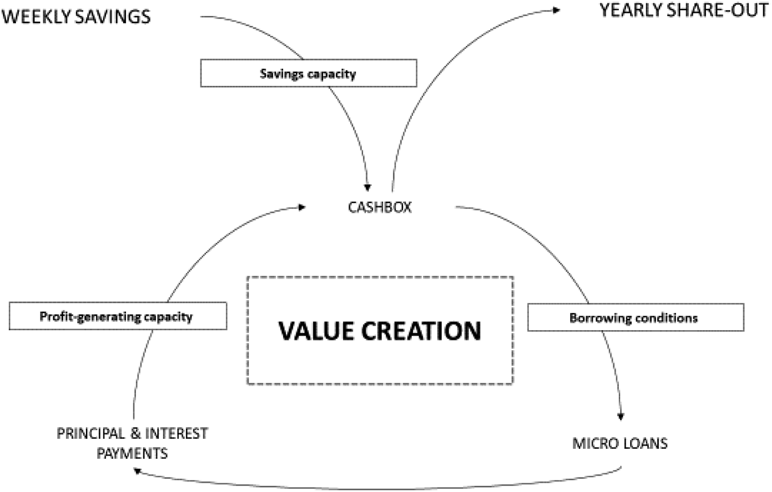
The savings capacity allows us to approximate the ability of the groups to mobilize savings from members. The importance of savings, as well as the fact that poor people do save, is well attested in the literature (Karlan et al., 2014; Prina, 2015). Additionally, a number of impact studies point out the positive impacts of micro-savings on income and asset indicators, whereas the impact of micro-credit remains contested (Banerjee et al., 2015; Tarozzi et al., 2015).
The profit-generating capacity allows us to approximate the ability of the groups to generate profits throughout the cycle. It indicates whether mobilized savings are efficiently used. As mentioned earlier, profits are primarily generated through interest payments on loans. Higher profit-generation thus occurs when at any given point, a higher proportion of the collected savings are lent on into interest-bearing loans. Productive lending by the SG-members i.e. using the loans for outside positive NPV-investment projects where the yield on investment is higher than the interest rate charged on the loan, is thus a necessary precondition for generating profits in the group that are shared-out at the end of the cycle
Finally, the borrowing conditions allows us to gain insight into the accessibility of SG loans to group members. In the context of microfinance, borrowing conditions have been amply discussed in the literature. For example, interest rates charged on micro-credit have been analyzed in several studies, triggering a debate on ethical interest rates (Hudon & Sandberg, 2013).
These three complementary performance dimensions capture the financial economics of the SG model. By quantifying these performance dimensions, both across and within cycles, we can get a comprehensive picture of the financial performance of SGs. In the next section, we look at the data provided by the SAVIX database and construct performance variables that will be used to analyze the different performance dimensions. We then present within- and across-cycle statistics and discuss the results.
Database and Construction of Performance Variables
The SAVIX Database
We construct our group-level statistics using data extracted from the Savings Groups Information Exchange (SAVIX). This is an initiative started by VSL Associates, a consortium of development actors actively involved in the promotion of the SG model. The database is funded by the Bill and Melinda Gates Foundation and international NGOs including CARE International, Catholic Relief Services, Oxfam International, and Plan International. It contains standardized quarterly information at the group level on SGs in 44 different countries. Around 89% of the SGs in our data are located in Africa, followed by Asia (8.5%) and the Americas (7.56%). The statistics reported in this paper summarize information from the first quarter of 2010 up to the last quarter of 2017 resulting in a database consisting of information on approximately 276,000 SGs.
The SAVIX collects variables related to group composition (e.g., the number of members, number of male/female members, etc.), group dynamics (e.g., dropout rate, meeting attendance rate, etc.), and group financial performance. Regarding the latter, the database keeps track of group assets (outstanding loans to group members, cash in the cashbox, cash in the social fund, cash in bank accounts, and group property) and group liabilities (outstanding savings, external debt, etc.).
Obviously, the database is not free from limitations. First, there is a possible selection bias in the sense that most SGs are initiated by external stakeholders and often under guidance of a facilitating development agency. Only a small proportion of SGs (4.8% of the observations) have no link to any development agency; i.e., they are ‘spontaneous groups’ that have replicated the model practiced by facilitated groups. This does not mean that facilitated groups always operate under the active guidance of a development agency. In general, facilitated groups ‘graduate’ from a development program and are left to their own management after around one year. In our data, around 19% of the observations entail groups that are self-managed, i.e., no longer actively guided. Nevertheless, the fact that most groups were originally initiated by external stakeholders means that groups that are not part of any development program are largely missing in the data. This is an important drawback, since the facilitated SG model represents only one specific type of SG. As mentioned, SGs are a complex and diverse phenomenon with a longstanding history in developing countries and we have to recognize that the wide heterogeneity of the SG-models is not represented in the SAVIX database. It must be emphasized that our insights apply specifically to facilitated SGs that are promoted by development agencies.
Second, the data is self-reported, which can lead to reporting problems. Typically, local field agents register the data. While this can be considered some form of ‘third-party’ check, it does not guarantee that the data is free from errors. Implementing strict data-cleaning procedures to avoid duplicate observations and outliers is therefore required.
Third, we mostly observe groups during their initial stage, i.e., at the start of their operations, which can lead to attrition bias. In the context of SGs, this problem is less pronounced because each consecutive cycle can be considered as a new starting point. In that sense, we observe consecutive SG operational stages and can therefore treat the data as an unbalanced pooled dataset where the group is the cross-section and the time dimension is a point in the cycle rather than an observed time period. Nevertheless, we still do not observe the long-term survival of the groups.
To control for sample attrition, we include both full-sample statistics and statistics on a subsample of SGs observed over a period of four consecutive cycles, i.e., groups that have ‘survived’ and have operated for at least four years. 2 This does not imply that the other groups in the database have ceased to exist. It is more likely that they are no longer visible in the data but have continued their operations autonomously. Because of the attrition bias, the number of observations in our data may differ, both across and within cycles. Some groups might be observed once per cycle, others twice or even more. However, as this problem is more pronounced in the full sample than in the subset of survivors, we only include ‘survivor groups’ in our results. The full-sample statistics can be found in the Appendix.
Variable Construction
With regard to savings capacity, we construct a savings per member per week variable, both unscaled and scaled by GNI per capita. We also construct a savings growth variable, which captures the percentage of growth in savings independently of the savings amount and hence of the economic situation of the members. These variables respectively measure the extent and speed with which savings are mobilized by SGs.
With regard to profit-generating capacity, we construct variables related to the fund utilization rate (FUR), which takes the value of outstanding loans and scales it by outstanding savings and total assets, respectively. These variables capture how actively savings are converted into loans. We also report statistics on a related variable that divides the number of loans by the number of members to capture the proportion of members that hold loans, which can be viewed as a non-monetary variant of the fund utilization rate. In addition, we construct a return on savings (ROS) variable, which captures all profit-generating mechanisms deployed by the group. ROS captures the return on the invested savings by dividing the total profits generated in the group at any given time by the average savings that were used to produce these profits. The total profits are constructed based on the liquidation value, which is the cash surplus that remains if an SG would be liquidated on the spot. Since all profits are shared out at the end of the cycle, calculating the percentage return on each dollar saved can be understood as a direct measure of wealth creation for SG members. This again under the assumption that the profits stemming from individual investments by SG members are at least as high as the interest rate charged on loans.
Regarding the borrowing conditions, we construct a proxy for the average loan size by dividing the value of outstanding loans by the number of outstanding loans. We report this ratio in dollar amounts both scaled and unscaled by GNI per capita. This variable offers insight into the size of the loans which can be compared to the size of the mobilized savings. This in turn sheds light on the economic opportunities that SG members can finance through their participation in the group. Additionally, we construct a proxy for the interest rate charged on loans, based on the changes in profits per dollar lent. We provide an estimate of the annualized changes in profit by dividing these changes by the value of outstanding loans (expressed on an annual basis). This yields an annualized percentage of the interest rate charged. This proxy assumes that loans are the sole profit-generating mechanism deployed by the group. However, as seen in the previous section this is not entirely correct as groups may also charge fines and penalties that generate additional profits. The interest rate proxy is therefore probably a slight overestimation of the actual interest rate charged on loans to members.
Variable Construction.
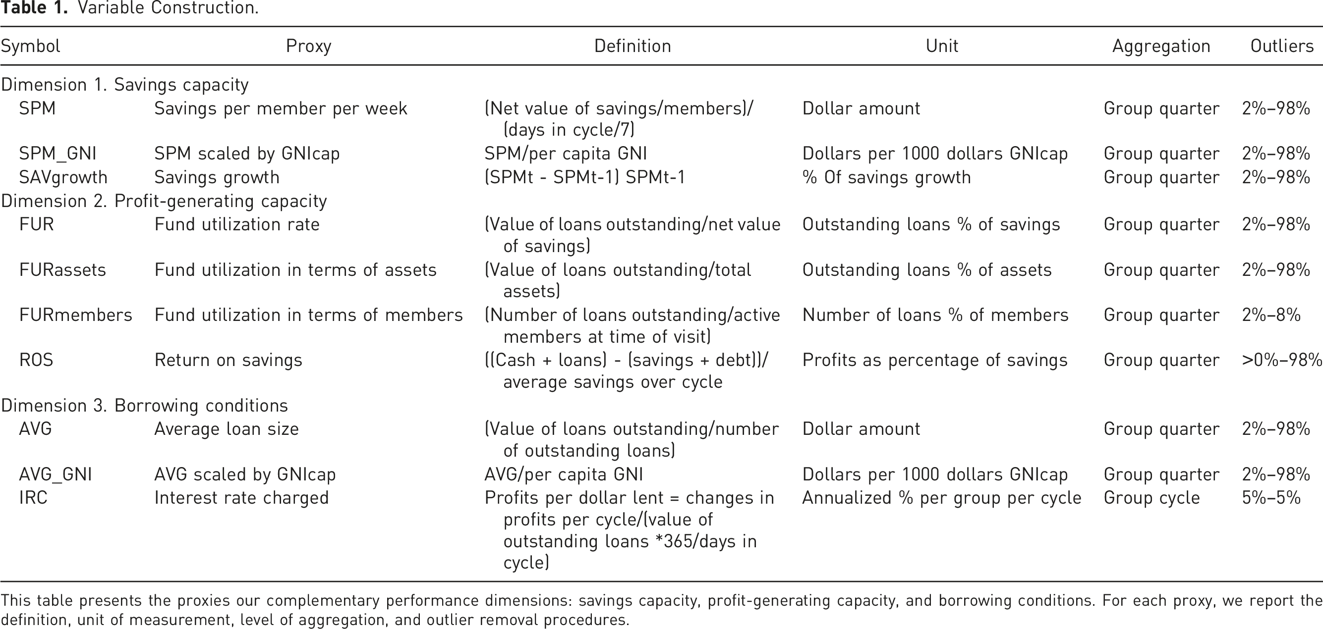
This table presents the proxies our complementary performance dimensions: savings capacity, profit-generating capacity, and borrowing conditions. For each proxy, we report the definition, unit of measurement, level of aggregation, and outlier removal procedures.
Results
To better control for attrition, we report statistics on the subset of ‘survivor groups,’ i.e., groups that have operated for at least four years. Full-sample statistics for all variables can be found in Appendix. Note however that our key findings are the same for both the full sample and the subset of survivors.
Savings Capacity.
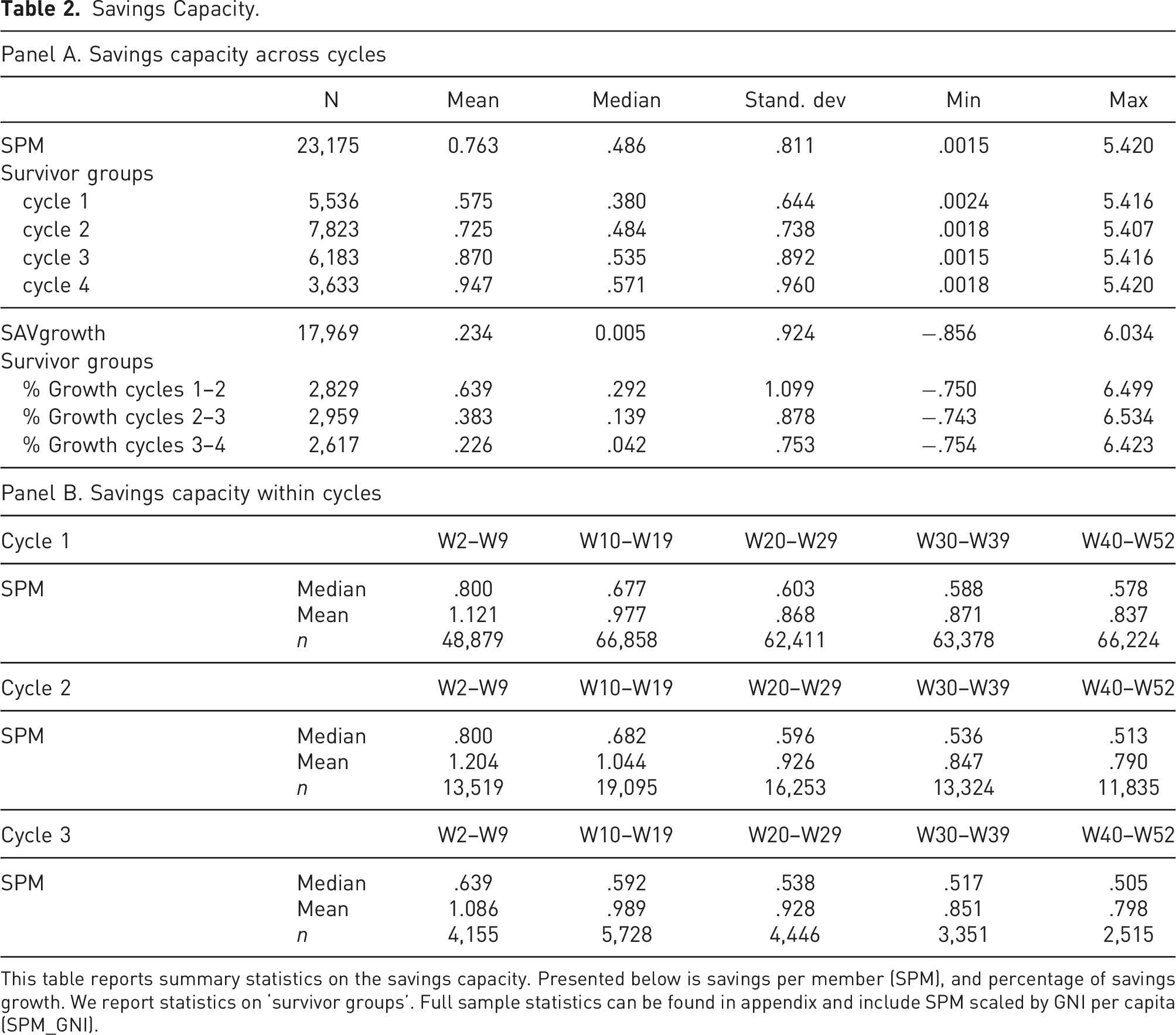
This table reports summary statistics on the savings capacity. Presented below is savings per member (SPM), and percentage of savings growth. We report statistics on ‘survivor groups’. Full sample statistics can be found in appendix and include SPM scaled by GNI per capita (SPM_GNI).
As can be seen in Panel A, median savings are 48 US dollar cents per member per week, while average savings are 76 US dollar cents per member per week. Hence, the term ‘micro-savings’ truly applies to the SG banking model. Looking at savings mobilization across cycles, we observe that both average and median savings steadily increase. Average savings are 57, 72, 87, and 94 US dollar cents per week in cycles 1, 2, 3, and 4, respectively. A repeated measures ANOVA rejects the null hypothesis of equal means at the 1% level, indicating that savings growth statistically differs across cycles. Our figures suggest that the savings capacity is steadily strengthened across cycles. This is confirmed when we look at the percentages of savings growth. We find that on average savings increase by 23% across the panel, with savings growth of 63% as groups move from cycle 1 to cycle 2, 38% from cycle 2 to cycle 3, and 22% from cycle 3 to cycle 4. Again, repeated measures ANOVA reject the null hypothesis of equal means at the 1% level.
Turning to within-cycle dynamics (Panel B) we see that members struggle to maintain their initial savings discipline, as weekly savings tend to go down as the cycle progresses. In cycle 1, for instance, it can be seen that, on average, weekly savings decline: 112 US dollar cents are saved per member per week (in weeks 2–9), 97 US dollar cents (in weeks 10–19), 86 US dollar cents (in weeks 20–29), 87 US dollar cents (in weeks 30–39), and 83 US dollar cents (in weeks 40–52). A similar pattern is observed in subsequent cycles. This decline can be explained by the SG operational model, notably the cycle system. As the cycle progresses, SG members often have lower amounts of surplus cash because loans have to be repaid. Members may also earn a seasonal income, making it hard to free up cash in periods of low income.
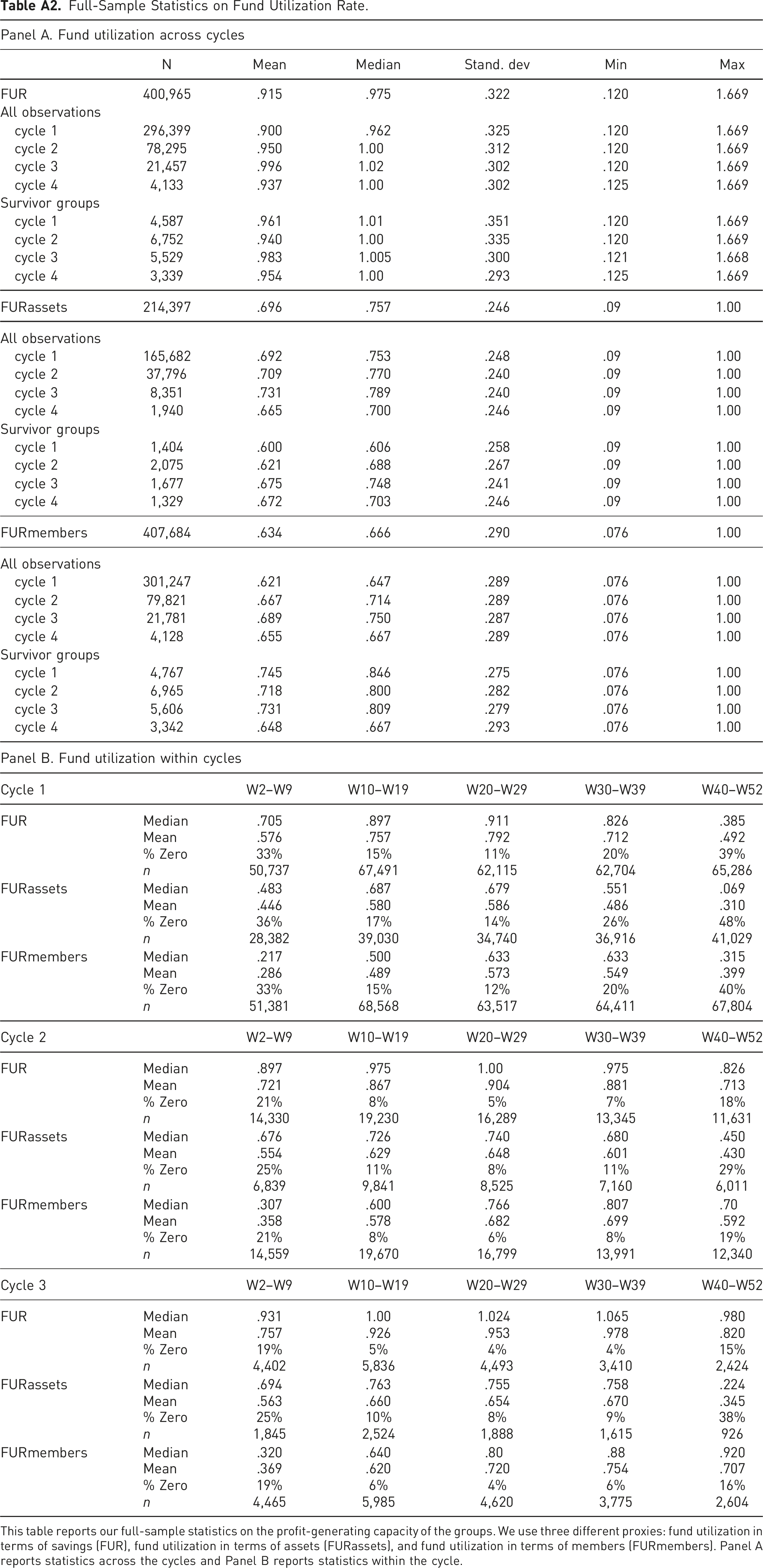
Fund Utilization Rate.
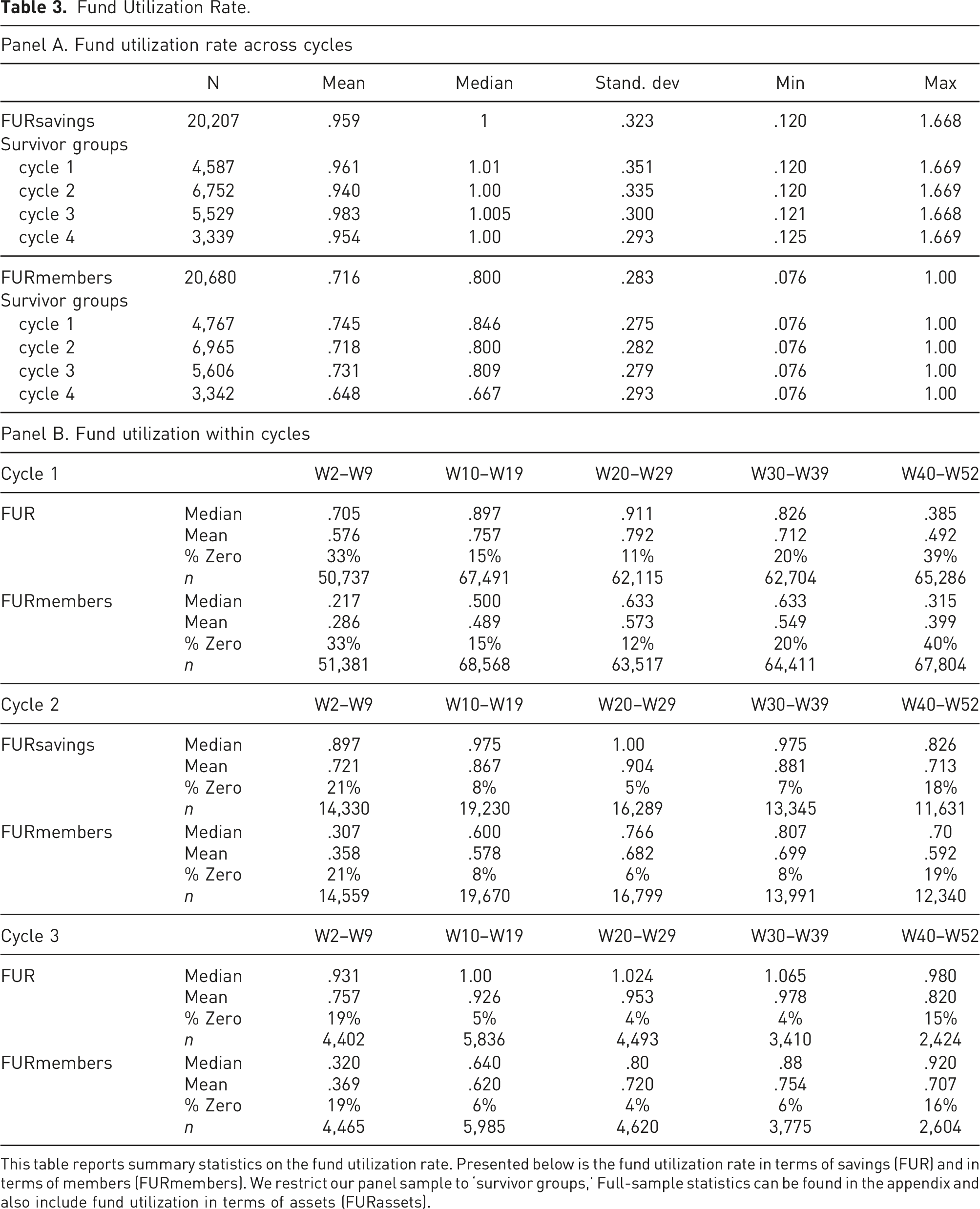
This table reports summary statistics on the fund utilization rate. Presented below is the fund utilization rate in terms of savings (FUR) and in terms of members (FURmembers). We restrict our panel sample to ‘survivor groups,’ Full-sample statistics can be found in the appendix and also include fund utilization in terms of assets (FURassets).
Return on Savings (ROS).
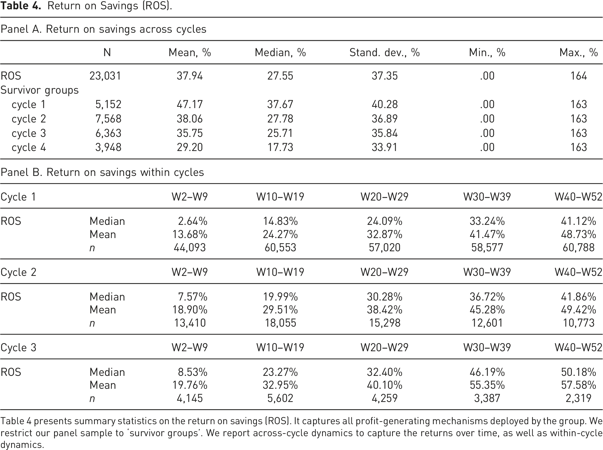
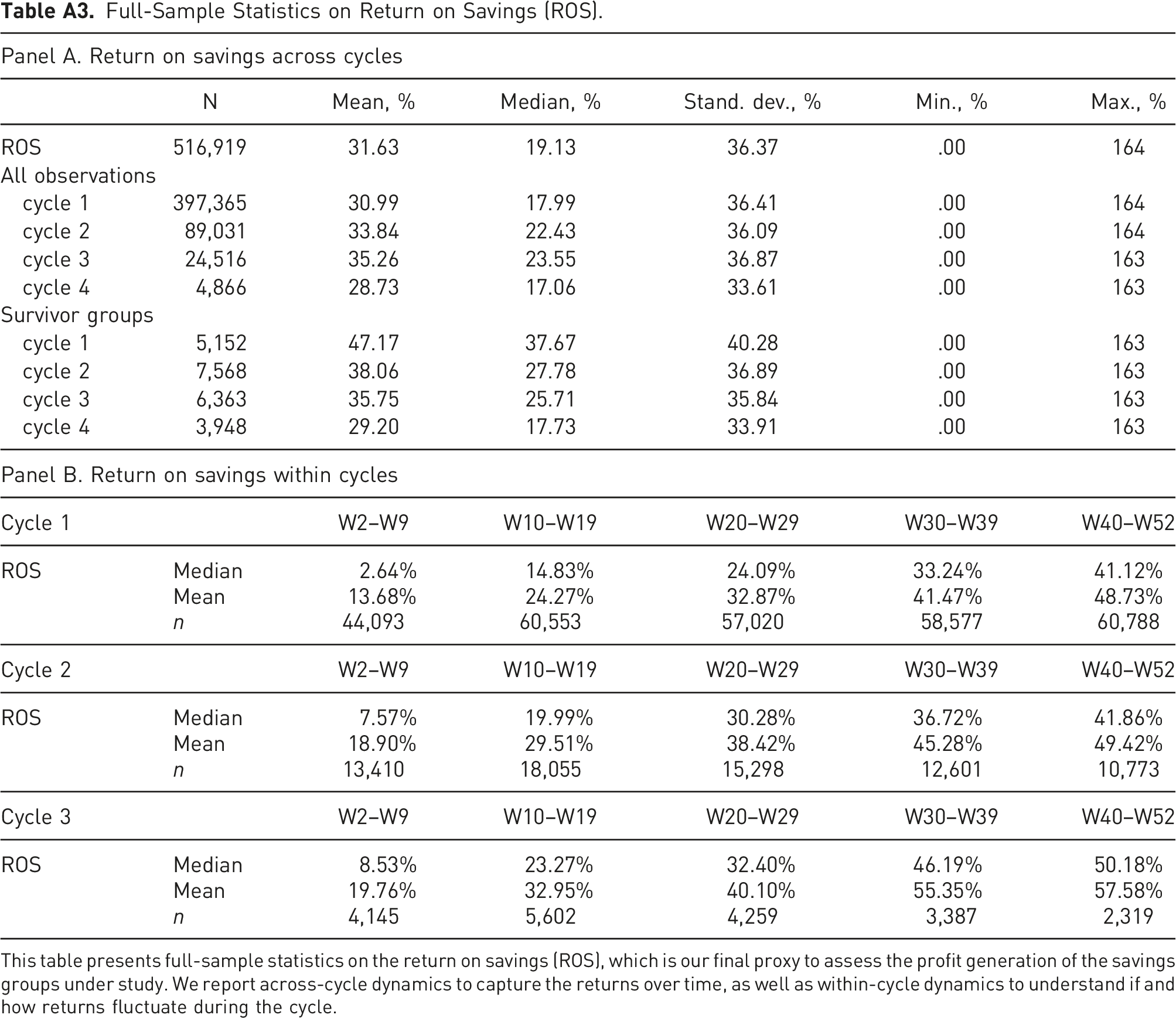
Table 4 presents summary statistics on the return on savings (ROS). It captures all profit-generating mechanisms deployed by the group. We restrict our panel sample to ‘survivor groups’. We report across-cycle dynamics to capture the returns over time, as well as within-cycle dynamics.
When analyzing the figures on fund utilization across cycles, several patterns emerge. First, we observe that on average across the panel, savings are actively converted into loans. On average, for each US dollar saved, .95 is converted into loans (FUR). This supports earlier findings by Burlando et al. (2021), that given the resource constraint posed by the funds available in the cash-box, FUR is close to 1. In terms of members, each member takes an average of .71 loans, which means that at any given point in time, some 71% of members hold loans and 29% do not. Comparing fund utilization across consecutive cycles, we find that fund utilization is remarkably stable and even slightly decreasing. There appears to be no increasing focus on profit generation via borrowing as groups move through their consecutive cycles. This might be explained by the fact that many groups ‘tie’ the amount of the loan of each member to the amount of the contributed savings. This imposes an upper bound on the issuance of productive loans and consequently on the profit-generating capacity.
Turning to within-cycle dynamics (Table 3, Panel B), we observe a clear pattern. At the start of the first cycle (weeks 2–9) fund utilization is low and 33% of the observations show zero outstanding loans. This indicates unproductive periods early in the cycle. This is not surprising, since funds must first accumulate before any lending can take place. Group productivity then increases gradually up until week 30, as savings are actively converted into loans. We report 11% zero outstanding loans between weeks 20 and 29. Toward the end of the cycle, productivity goes down again, as loans are recovered for the share-out. We report 39% zero outstanding loans between weeks 40 and 52. Consequently, within-cycle dynamics reveal an inverted U-shaped pattern, with low fund utilization at the start and end of the cycle, and high fund utilization in between.
In cycles 2 and 3, a similar pattern is observed. For a substantial part of the cycle, and notably at the start and end of the cycle, loans are not issued, which constrains the profit-generating capacity of the groups. However, there seems to be a learning effect in the sense that as groups move from one cycle to another, productivity is generally higher as they mobilize a bigger share of the savings earlier in the cycle. For instance, in cycle 1 around 33% of the observations show zero outstanding loans and around 57% of savings are converted into loans, whereas in cycles 2 and 3, respectively, 21% and 19% of the observations show zero outstanding loans and 72% and 75% of savings are converted into loans. This is in line with the notion that social capital in the form of trust is built among SG members gradually (Allan & Panetta, 2010).
Table 4 reports the return on savings (ROS), defined as total profits as a percentage of average savings both across cycles (Panel A) and within the cycle (Panel B). The ROS is quite high across the whole panel (nearly 38% on average). This shows that although groups mobilize low savings amounts and have unproductive periods, quite substantial returns are realized. However, when analyzing the ROS across different cycles, we see a declining pattern. For instance, the average ROS is 47%, 38%, and 36% in cycles 1, 2, and 3, respectively, and then drops to 29% in cycle 4. This pattern is even more pronounced for the median, with a ROS of 38%, 28%, 26%, and 18% in cycles 1 to 4, respectively. Following a repeated measures ANOVA, the null hypothesis of equal means is again rejected at the 1% level.
Turning to within-cycle dynamics, we find that the ROS steadily increases throughout the cycle. In cycle 1, the average ROS increases from 13.68% (weeks 2–9) to 32.87% (weeks 20–29) to 48.73% (weeks 40–52). In cycles 2 and 3, a similar pattern is observed. In addition, the average ROS appears to be higher in cycles 2 and 3 compared to cycle 1. This again suggests the notion of social capital and trust being built up as groups mature, resulting in a lower share of unproductive savings early in the cycle.
Borrowing Conditions.
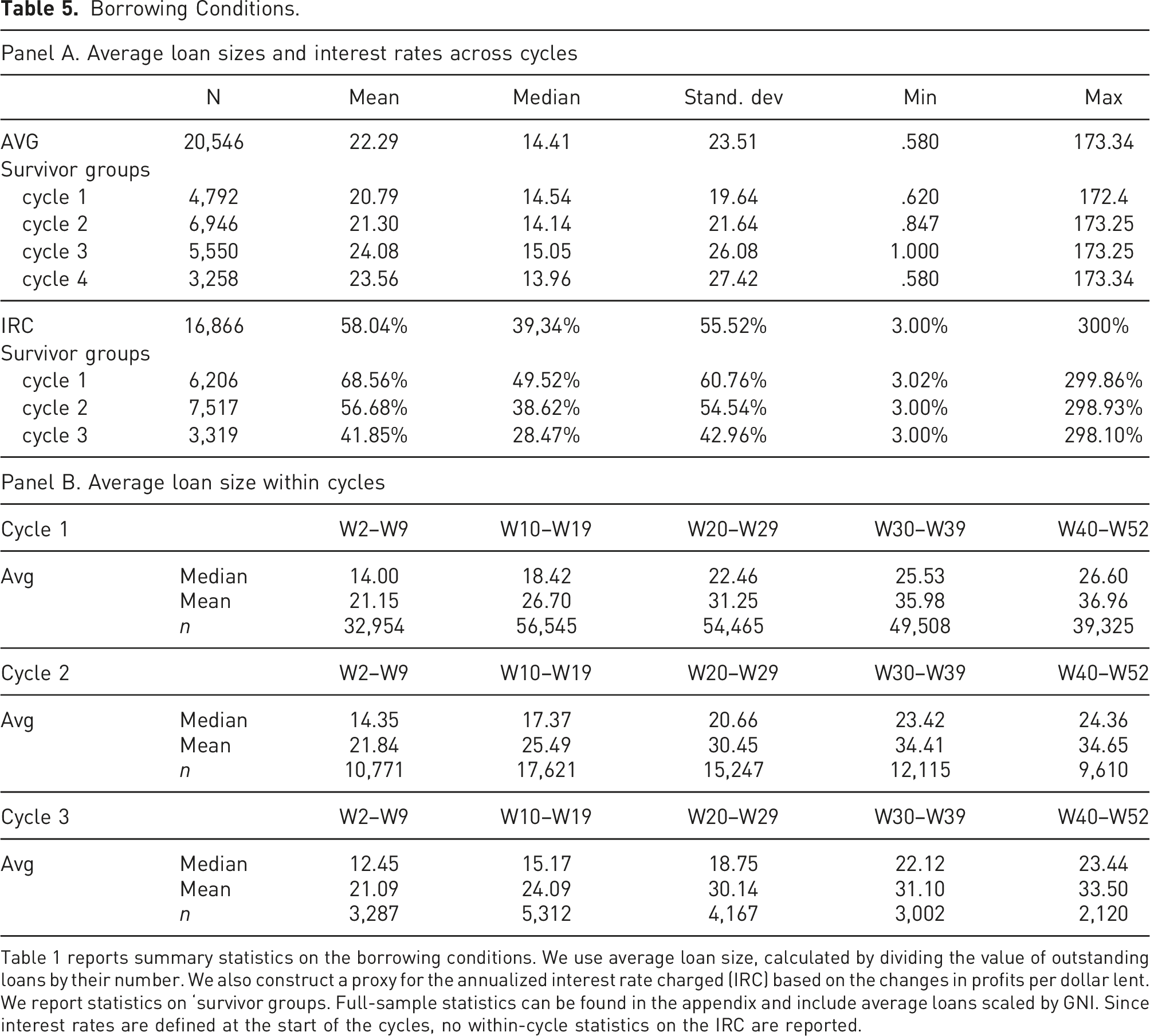
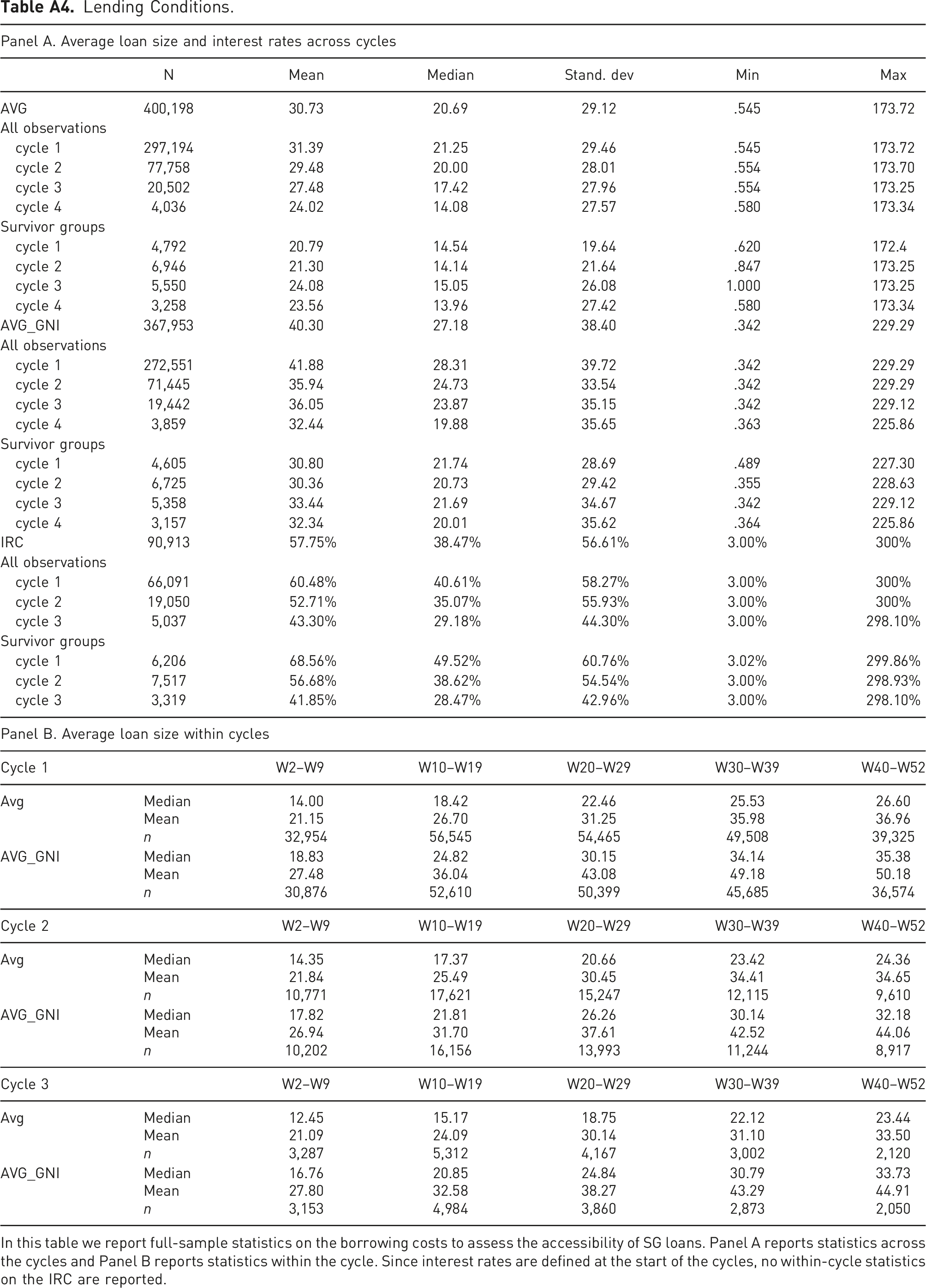
Table 1 reports summary statistics on the borrowing conditions. We use average loan size, calculated by dividing the value of outstanding loans by their number. We also construct a proxy for the annualized interest rate charged (IRC) based on the changes in profits per dollar lent. We report statistics on ‘survivor groups. Full-sample statistics can be found in the appendix and include average loans scaled by GNI. Since interest rates are defined at the start of the cycles, no within-cycle statistics on the IRC are reported.
We observe that the average loan amount is 22.29 US dollars (14.41 US dollars for the median) across the whole panel (Panel A). It can be seen that loan amounts are small but stable as groups move through consecutive cycles. For instance, looking at average loan amounts across cycles, we find 20 US dollars for cycle 1, 21 US dollars for cycle 2, and 24 US dollars for cycle 3, and 23 US dollars for cycle 4. Repeated measures ANOVA results allow us to reject the null hypothesis of equal means at the 1% level.
In Panel B, we observe a clear within-cycle pattern: average loans increase throughout the cycle. In the first cycle, for instance, it can be seen that the average loan size in the median group is $14, $18, $22, $25, and $26 in weeks 10, 20, 30, 40, and 52, respectively. The same within-cycle pattern is observed in cycles 2 and 3. While this may reflect an increase in demand for loans, it more likely reflects an increase in members’ contributed savings, which are a precondition for borrowing money, i.e., ‘loan-tying’. As members build up their savings balance throughout the cycle, their individual borrowing constraints are relaxed, enabling them to access somewhat larger loans.
Looking at the interest rate charged (IRC), estimated as annualized changes in profits per dollar lent, we observe that borrowers are charged on average around 58% annually across the panel. The median group is charged around 39% annually, which is slightly less than 1% per week. However, we see that interest rates decline consistently. On average, interest rates go down from 68% to 56% to 41% in cycles 1, 2, and 3, respectively. A similar pattern is observed in the median group. A repeated measures ANOVA confirms that means are different across cycles. 3 Groups seem to settle for lower interest rates as they move through consecutive cycles. This may reflect that groups consider standard interest rates suggested by facilitating agencies too high. Groups would then opt for lower interest rates as they grow independent of the facilitating agency. It may also reflect social capital and trust being built up, allowing to demand a lower risk premium and interest rates to drop. It is clear however, that there is a tradeoff between lower interest rates and higher profit generation.
Overall and combined, our statistics suggest that loans are predominantly used to smooth out unexpected expenses or in case of emergencies, i.e. cash-management purposes. The profit-generating capacity is curtailed by implementation restrictions, notably unproductive periods and the cycle system, that impede the potential of members to leverage long-term profitable investments via SGs. 4
Conclusion
Development agencies are increasingly promoting member-based SGs but struggle to evaluate their financial performance. In this paper, we treat SGs as microeconomic entities and construct global comparative statistics on three complementary financial performance dimensions. We investigate the savings capacity and profit-generating capacity of the groups as well as the borrowing conditions imposed. Based on a novel global dataset, i.e. the SAVIX, we construct variables that allow us to analyze these performance dimensions. We report within-cycle and across-cycles statistics to uncover restrictions inherent in the SG implementation model and to investigate the financial potential of SGs at the global level.
Our findings can be summarized as follows. We find strong positive growth in savings as groups move through consecutive cycles. Although weekly savings amounts are small, we observe a steady increase in savings capacity across cycles and a positive concave growth in savings (23% on average across the panel). Within each cycle, however, members struggle to maintain their savings discipline when they start to take out loans. Since many members earn a seasonal income, savings might also decrease in periods of low income.
With regard to profit-generating capacity, our findings do not suggest an increasing focus on profit generation as groups move through consecutive cycles. Fund utilization is remarkably stable, suggesting that profit generation is curtailed by the cycle model where members first need to save up funds before accessing loans. Similarly, members are prohibited from borrowing toward the end of the cycle. This is evidenced by the unproductive periods, notably at the start and end of the cycle. However, there seems to be a ‘learning effect’, as unproductive periods become shorter across consecutive cycles. This is consistent with the notion of social capital and trust being built up as groups mature. Returns on savings are substantial, in the magnitude of 38% on average and 27% in the median group. However, these returns steadily decline across cycles, reconfirming that profit generation is curtailed by the annual cycle model.
On the lending side, we observe that loans are small (22 dollars on average). Estimated annual interest rate are 58% on average and 39% for the median. As groups mature, groups generally opt for lower interest rates, which leads to a decrease in profits that can be shared out. This is consistent with a preference for more favorable borrowing conditions at the individual level over wealth creation at the group level. Groups seem to prefer affordable small-scale loans over maximizing profit generation.
Overall, our statistics suggest that SGs are predominantly used as cash-management vehicles to balance out asymmetric income and unexpected expenses, i.e., emergency lending. By stimulating the poor to save regularly and address cash-flow issues, SGs offer an important liquidity safety net. However, the profit-generating capacity is curtailed by two major implementation restrictions, namely, the tying of loans to members’ savings and the unproductive periods inherent to the cycle model. These restrictions impede the potential of members to leverage long-term profitable investments via SGs.
Our findings raise some important implications. Should donors settle for the objective of cash management or should they revise their implementation model to enable greater profit generation? Improving the profit-generating capacity of the group means increasing its fund utilization. Burlando et al. (2021) refer in this regard to restricted resource availability, since groups are tied to the money available in the cash-box. From a financial perspective however, relaxing the personal borrowing constraint (i.e. each member first needs to save three times their respective loan amount) by allowing more lending per dollar saved could increase financial efficiency and stimulate long-term productive investments. Another way to enhance financial efficiency would be to move from a yearly share-out to longer cycles (with possible intermediate share-outs of accumulated interest). This would lower the emphasis on loan repayment and minimize the occurrence of unproductive periods where no lending takes place.
However, several tradeoffs need to be considered. Since SG members their income is subject to considerable fluctuations, smoothing irregular income patterns remains vital (Mersland & Eggen, 2007). Also, as stated by Jones and Kalmi (2009), the importance of cooperatives is not solely derived from their economic significance, but also because of their ability to address market failures. In this regard, SGs address a demand from a specific target group, i.e., poor households excluded from financial intermediation services. One could argue that SGs create necessary socioeconomic preconditions for members to create wealth from external opportunities. Future research is needed to explore this in more detail, for example, by studying whether SG membership can leverage or diminish the impact of formal credit via MFIs.
Donors should assess how the SG banking model relates to other microfinance initiatives and through which channels SGs can contribute to financial inclusion. Given the reciprocity-based logic associated with the cooperative SG model, attention should be paid to the feasibility of introducing measures that increase profit generation.
Footnotes
Declaration of Conflicting Interests
The author(s) declared no potential conflicts of interest with respect to the research, authorship, and/or publication of this article.
Funding
The author(s) disclosed receipt of the following financial support for the research, authorship, and/or publication of this article: This work was supported by the Fonds Wetenschappelijk Onderzoek grant no G067820H, S006019N.
Notes
Appendix
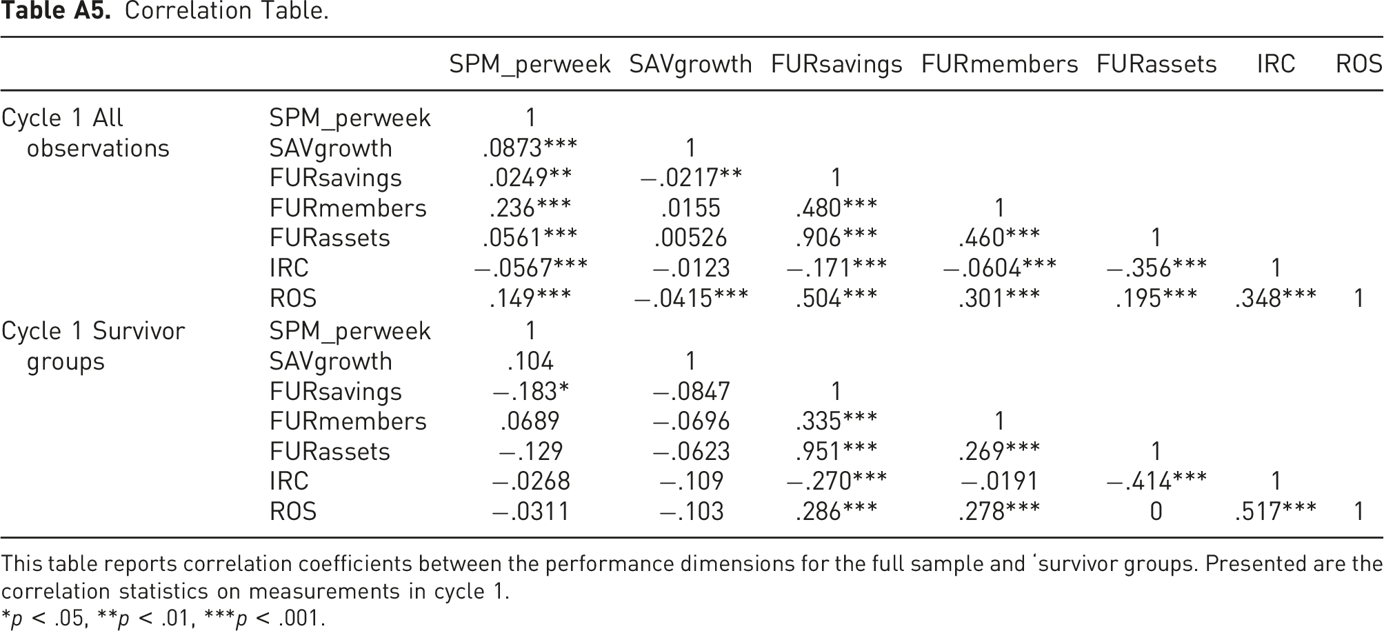
Full-Sample Statistics on Savings Capacity. This table reports full-sample statistics on the savings capacity of the groups. We use the savings per member per week, both unscaled and scaled by GNI, as well as the savings growth as proxies. Panel A reports statistics across the cycles and Panel B reports statistics within the cycle. Full-Sample Statistics on Fund Utilization Rate. This table reports our full-sample statistics on the profit-generating capacity of the groups. We use three different proxies: fund utilization in terms of savings (FUR), fund utilization in terms of assets (FURassets), and fund utilization in terms of members (FURmembers). Panel A reports statistics across the cycles and Panel B reports statistics within the cycle. Full-Sample Statistics on Return on Savings (ROS). This table presents full-sample statistics on the return on savings (ROS), which is our final proxy to assess the profit generation of the savings groups under study. We report across-cycle dynamics to capture the returns over time, as well as within-cycle dynamics to understand if and how returns fluctuate during the cycle. Lending Conditions. In this table we report full-sample statistics on the borrowing costs to assess the accessibility of SG loans. Panel A reports statistics across the cycles and Panel B reports statistics within the cycle. Since interest rates are defined at the start of the cycles, no within-cycle statistics on the IRC are reported. Correlation Table. This table reports correlation coefficients between the performance dimensions for the full sample and ‘survivor groups. Presented are the correlation statistics on measurements in cycle 1. *p < .05, **p < .01, ***p < .001.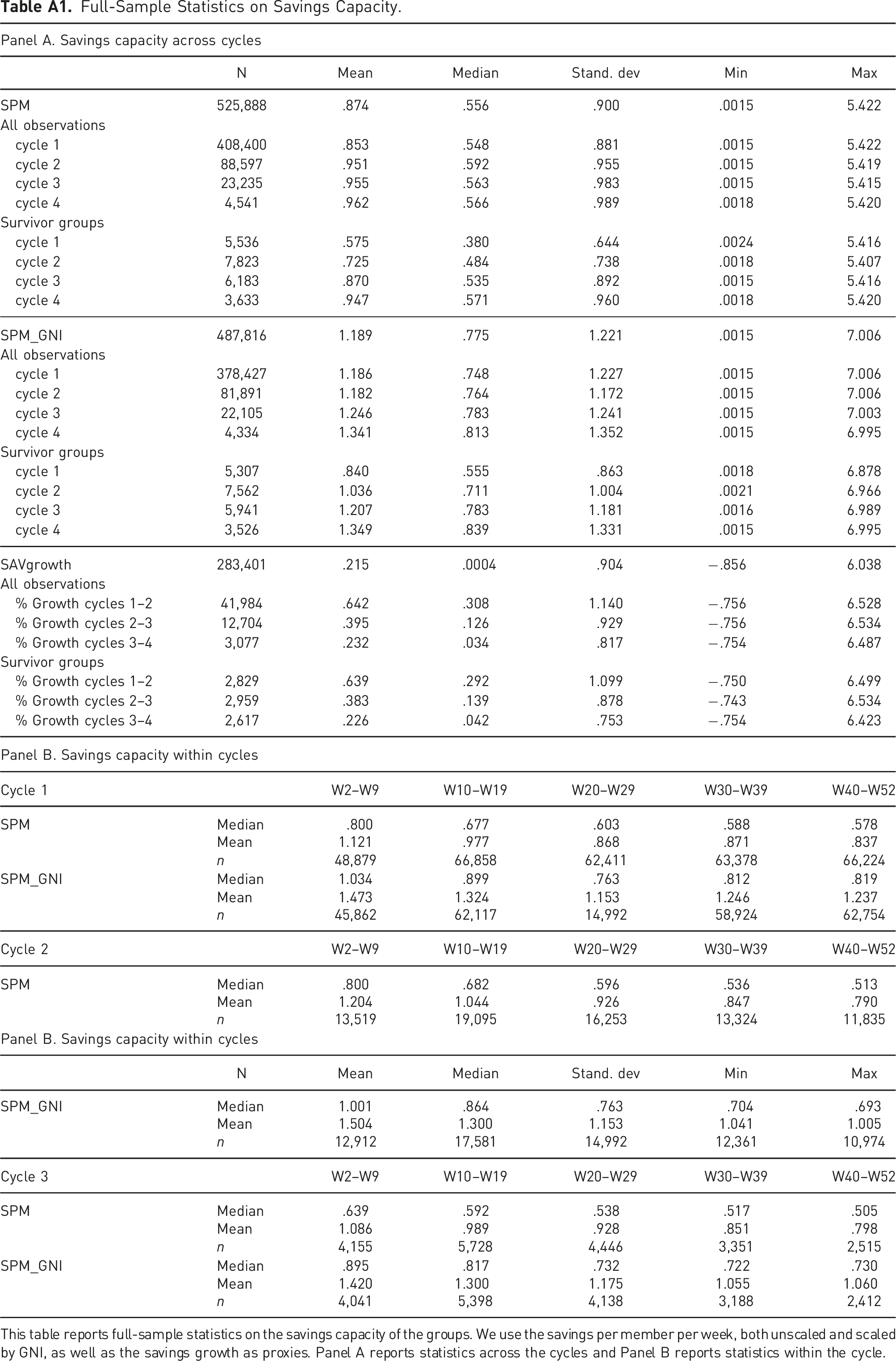
Panel A. Savings capacity across cycles
N
Mean
Median
Stand. dev
Min
Max
SPM
525,888
.874
.556
.900
.0015
5.422
All observations
cycle 1
408,400
.853
.548
.881
.0015
5.422
cycle 2
88,597
.951
.592
.955
.0015
5.419
cycle 3
23,235
.955
.563
.983
.0015
5.415
cycle 4
4,541
.962
.566
.989
.0018
5.420
Survivor groups
cycle 1
5,536
.575
.380
.644
.0024
5.416
cycle 2
7,823
.725
.484
.738
.0018
5.407
cycle 3
6,183
.870
.535
.892
.0015
5.416
cycle 4
3,633
.947
.571
.960
.0018
5.420
SPM_GNI
487,816
1.189
.775
1.221
.0015
7.006
All observations
cycle 1
378,427
1.186
.748
1.227
.0015
7.006
cycle 2
81,891
1.182
.764
1.172
.0015
7.006
cycle 3
22,105
1.246
.783
1.241
.0015
7.003
cycle 4
4,334
1.341
.813
1.352
.0015
6.995
Survivor groups
cycle 1
5,307
.840
.555
.863
.0018
6.878
cycle 2
7,562
1.036
.711
1.004
.0021
6.966
cycle 3
5,941
1.207
.783
1.181
.0016
6.989
cycle 4
3,526
1.349
.839
1.331
.0015
6.995
SAVgrowth
283,401
.215
.0004
.904
−.856
6.038
All observations
% Growth cycles 1–2
41,984
.642
.308
1.140
−.756
6.528
% Growth cycles 2–3
12,704
.395
.126
.929
−.756
6.534
% Growth cycles 3–4
3,077
.232
.034
.817
−.754
6.487
Survivor groups
% Growth cycles 1–2
2,829
.639
.292
1.099
−.750
6.499
% Growth cycles 2–3
2,959
.383
.139
.878
−.743
6.534
% Growth cycles 3–4
2,617
.226
.042
.753
−.754
6.423
Panel B. Savings capacity within cycles
Cycle 1
W2–W9
W10–W19
W20–W29
W30–W39
W40–W52
SPM
Median
.800
.677
.603
.588
.578
Mean
1.121
.977
.868
.871
.837
n
48,879
66,858
62,411
63,378
66,224
SPM_GNI
Median
1.034
.899
.763
.812
.819
Mean
1.473
1.324
1.153
1.246
1.237
n
45,862
62,117
14,992
58,924
62,754
Cycle 2
W2–W9
W10–W19
W20–W29
W30–W39
W40–W52
SPM
Median
.800
.682
.596
.536
.513
Mean
1.204
1.044
.926
.847
.790
n
13,519
19,095
16,253
13,324
11,835
Panel B. Savings capacity within cycles
N
Mean
Median
Stand. dev
Min
Max
SPM_GNI
Median
1.001
.864
.763
.704
.693
Mean
1.504
1.300
1.153
1.041
1.005
n
12,912
17,581
14,992
12,361
10,974
Cycle 3
W2–W9
W10–W19
W20–W29
W30–W39
W40–W52
SPM
Median
.639
.592
.538
.517
.505
Mean
1.086
.989
.928
.851
.798
n
4,155
5,728
4,446
3,351
2,515
SPM_GNI
Median
.895
.817
.732
.722
.730
Mean
1.420
1.300
1.175
1.055
1.060
n
4,041
5,398
4,138
3,188
2,412
Panel A. Fund utilization across cycles
N
Mean
Median
Stand. dev
Min
Max
FUR
400,965
.915
.975
.322
.120
1.669
All observations
cycle 1
296,399
.900
.962
.325
.120
1.669
cycle 2
78,295
.950
1.00
.312
.120
1.669
cycle 3
21,457
.996
1.02
.302
.120
1.669
cycle 4
4,133
.937
1.00
.302
.125
1.669
Survivor groups
cycle 1
4,587
.961
1.01
.351
.120
1.669
cycle 2
6,752
.940
1.00
.335
.120
1.669
cycle 3
5,529
.983
1.005
.300
.121
1.668
cycle 4
3,339
.954
1.00
.293
.125
1.669
FURassets
214,397
.696
.757
.246
.09
1.00
All observations
cycle 1
165,682
.692
.753
.248
.09
1.00
cycle 2
37,796
.709
.770
.240
.09
1.00
cycle 3
8,351
.731
.789
.240
.09
1.00
cycle 4
1,940
.665
.700
.246
.09
1.00
Survivor groups
cycle 1
1,404
.600
.606
.258
.09
1.00
cycle 2
2,075
.621
.688
.267
.09
1.00
cycle 3
1,677
.675
.748
.241
.09
1.00
cycle 4
1,329
.672
.703
.246
.09
1.00
FURmembers
407,684
.634
.666
.290
.076
1.00
All observations
cycle 1
301,247
.621
.647
.289
.076
1.00
cycle 2
79,821
.667
.714
.289
.076
1.00
cycle 3
21,781
.689
.750
.287
.076
1.00
cycle 4
4,128
.655
.667
.289
.076
1.00
Survivor groups
cycle 1
4,767
.745
.846
.275
.076
1.00
cycle 2
6,965
.718
.800
.282
.076
1.00
cycle 3
5,606
.731
.809
.279
.076
1.00
cycle 4
3,342
.648
.667
.293
.076
1.00
Panel B. Fund utilization within cycles
Cycle 1
W2–W9
W10–W19
W20–W29
W30–W39
W40–W52
FUR
Median
.705
.897
.911
.826
.385
Mean
.576
.757
.792
.712
.492
% Zero
33%
15%
11%
20%
39%
n
50,737
67,491
62,115
62,704
65,286
FURassets
Median
.483
.687
.679
.551
.069
Mean
.446
.580
.586
.486
.310
% Zero
36%
17%
14%
26%
48%
n
28,382
39,030
34,740
36,916
41,029
FURmembers
Median
.217
.500
.633
.633
.315
Mean
.286
.489
.573
.549
.399
% Zero
33%
15%
12%
20%
40%
n
51,381
68,568
63,517
64,411
67,804
Cycle 2
W2–W9
W10–W19
W20–W29
W30–W39
W40–W52
FUR
Median
.897
.975
1.00
.975
.826
Mean
.721
.867
.904
.881
.713
% Zero
21%
8%
5%
7%
18%
n
14,330
19,230
16,289
13,345
11,631
FURassets
Median
.676
.726
.740
.680
.450
Mean
.554
.629
.648
.601
.430
% Zero
25%
11%
8%
11%
29%
n
6,839
9,841
8,525
7,160
6,011
FURmembers
Median
.307
.600
.766
.807
.70
Mean
.358
.578
.682
.699
.592
% Zero
21%
8%
6%
8%
19%
n
14,559
19,670
16,799
13,991
12,340
Cycle 3
W2–W9
W10–W19
W20–W29
W30–W39
W40–W52
FUR
Median
.931
1.00
1.024
1.065
.980
Mean
.757
.926
.953
.978
.820
% Zero
19%
5%
4%
4%
15%
n
4,402
5,836
4,493
3,410
2,424
FURassets
Median
.694
.763
.755
.758
.224
Mean
.563
.660
.654
.670
.345
% Zero
25%
10%
8%
9%
38%
n
1,845
2,524
1,888
1,615
926
FURmembers
Median
.320
.640
.80
.88
.920
Mean
.369
.620
.720
.754
.707
% Zero
19%
6%
4%
6%
16%
n
4,465
5,985
4,620
3,775
2,604
Panel A. Return on savings across cycles
N
Mean, %
Median, %
Stand. dev., %
Min., %
Max., %
ROS
516,919
31.63
19.13
36.37
.00
164
All observations
cycle 1
397,365
30.99
17.99
36.41
.00
164
cycle 2
89,031
33.84
22.43
36.09
.00
164
cycle 3
24,516
35.26
23.55
36.87
.00
163
cycle 4
4,866
28.73
17.06
33.61
.00
163
Survivor groups
cycle 1
5,152
47.17
37.67
40.28
.00
163
cycle 2
7,568
38.06
27.78
36.89
.00
163
cycle 3
6,363
35.75
25.71
35.84
.00
163
cycle 4
3,948
29.20
17.73
33.91
.00
163
Panel B. Return on savings within cycles
Cycle 1
W2–W9
W10–W19
W20–W29
W30–W39
W40–W52
ROS
Median
2.64%
14.83%
24.09%
33.24%
41.12%
Mean
13.68%
24.27%
32.87%
41.47%
48.73%
n
44,093
60,553
57,020
58,577
60,788
Cycle 2
W2–W9
W10–W19
W20–W29
W30–W39
W40–W52
ROS
Median
7.57%
19.99%
30.28%
36.72%
41.86%
Mean
18.90%
29.51%
38.42%
45.28%
49.42%
n
13,410
18,055
15,298
12,601
10,773
Cycle 3
W2–W9
W10–W19
W20–W29
W30–W39
W40–W52
ROS
Median
8.53%
23.27%
32.40%
46.19%
50.18%
Mean
19.76%
32.95%
40.10%
55.35%
57.58%
n
4,145
5,602
4,259
3,387
2,319
Panel A. Average loan size and interest rates across cycles
N
Mean
Median
Stand. dev
Min
Max
AVG
400,198
30.73
20.69
29.12
.545
173.72
All observations
cycle 1
297,194
31.39
21.25
29.46
.545
173.72
cycle 2
77,758
29.48
20.00
28.01
.554
173.70
cycle 3
20,502
27.48
17.42
27.96
.554
173.25
cycle 4
4,036
24.02
14.08
27.57
.580
173.34
Survivor groups
cycle 1
4,792
20.79
14.54
19.64
.620
172.4
cycle 2
6,946
21.30
14.14
21.64
.847
173.25
cycle 3
5,550
24.08
15.05
26.08
1.000
173.25
cycle 4
3,258
23.56
13.96
27.42
.580
173.34
AVG_GNI
367,953
40.30
27.18
38.40
.342
229.29
All observations
cycle 1
272,551
41.88
28.31
39.72
.342
229.29
cycle 2
71,445
35.94
24.73
33.54
.342
229.29
cycle 3
19,442
36.05
23.87
35.15
.342
229.12
cycle 4
3,859
32.44
19.88
35.65
.363
225.86
Survivor groups
cycle 1
4,605
30.80
21.74
28.69
.489
227.30
cycle 2
6,725
30.36
20.73
29.42
.355
228.63
cycle 3
5,358
33.44
21.69
34.67
.342
229.12
cycle 4
3,157
32.34
20.01
35.62
.364
225.86
IRC
90,913
57.75%
38.47%
56.61%
3.00%
300%
All observations
cycle 1
66,091
60.48%
40.61%
58.27%
3.00%
300%
cycle 2
19,050
52.71%
35.07%
55.93%
3.00%
300%
cycle 3
5,037
43.30%
29.18%
44.30%
3.00%
298.10%
Survivor groups
cycle 1
6,206
68.56%
49.52%
60.76%
3.02%
299.86%
cycle 2
7,517
56.68%
38.62%
54.54%
3.00%
298.93%
cycle 3
3,319
41.85%
28.47%
42.96%
3.00%
298.10%
Panel B. Average loan size within cycles
Cycle 1
W2–W9
W10–W19
W20–W29
W30–W39
W40–W52
Avg
Median
14.00
18.42
22.46
25.53
26.60
Mean
21.15
26.70
31.25
35.98
36.96
n
32,954
56,545
54,465
49,508
39,325
AVG_GNI
Median
18.83
24.82
30.15
34.14
35.38
Mean
27.48
36.04
43.08
49.18
50.18
n
30,876
52,610
50,399
45,685
36,574
Cycle 2
W2–W9
W10–W19
W20–W29
W30–W39
W40–W52
Avg
Median
14.35
17.37
20.66
23.42
24.36
Mean
21.84
25.49
30.45
34.41
34.65
n
10,771
17,621
15,247
12,115
9,610
AVG_GNI
Median
17.82
21.81
26.26
30.14
32.18
Mean
26.94
31.70
37.61
42.52
44.06
n
10,202
16,156
13,993
11,244
8,917
Cycle 3
W2–W9
W10–W19
W20–W29
W30–W39
W40–W52
Avg
Median
12.45
15.17
18.75
22.12
23.44
Mean
21.09
24.09
30.14
31.10
33.50
n
3,287
5,312
4,167
3,002
2,120
AVG_GNI
Median
16.76
20.85
24.84
30.79
33.73
Mean
27.80
32.58
38.27
43.29
44.91
n
3,153
4,984
3,860
2,873
2,050
SPM_perweek
SAVgrowth
FURsavings
FURmembers
FURassets
IRC
ROS
Cycle 1 All observations
SPM_perweek
1
SAVgrowth
.0873***
1
FURsavings
.0249**
−.0217**
1
FURmembers
.236***
.0155
.480***
1
FURassets
.0561***
.00526
.906***
.460***
1
IRC
−.0567***
−.0123
−.171***
−.0604***
−.356***
1
ROS
.149***
−.0415***
.504***
.301***
.195***
.348***
1
Cycle 1 Survivor groups
SPM_perweek
1
SAVgrowth
.104
1
FURsavings
−.183*
−.0847
1
FURmembers
.0689
−.0696
.335***
1
FURassets
−.129
−.0623
.951***
.269***
1
IRC
−.0268
−.109
−.270***
−.0191
−.414***
1
ROS
−.0311
−.103
.286***
.278***
0
.517***
1