Sage Journals: Discover world-class research

Abstract

This study presents an alternative methodology for analyzing the difference in daily solar energy generation between two grid-connected photovoltaic arrays (PVAs) that are identical in capacity, technical characteristics, and have the same energy production measurement interval but are in two different municipalities of Mexico City (CDMX). Unlike conventional approaches, which often rely on environmental variables, this work proposes combining the cubic smoothing Spline technique with the separation of trend, seasonality, and cyclicality (TSCI) effects. The first technique reduces random variations in measurement, while the second separates the effects commonly found in time series data. The results obtained are useful for installers of this technology, as they allow them to determine in which borough a greater photovoltaic capacity is needed.

Keywords

optimization reference frame solar resource sum of squared time series decomposition

1. Introduction

Renewable energy plays a crucial role in the transition to cleaner energy, responsible for more than a third of the projected emissions reductions between 2020 and 2030 under the 2050 Net Zero Emissions Scenario. According to the International Energy Agency (IEA), 95% of the increase in global electrical capacity is expected to come from renewable sources, with solar photovoltaics contributing more than 50% (IEA 2024). In 2022, utility-scale plants were responsible for approximately half of global solar PV capacity additions (643 GW), followed by residential segments (195 GW) and commercial and industrial sectors (298 GW) (IEA 2023).

Grid-tied PV systems have gained popularity among residential users looking to reduce their energy consumption, but their intermittent nature due to environmental factors presents challenges in accurately sourcing the energy generated. Various methodologies and variables are used to estimate the energy and reliability of these systems. In (Fabara et al. 2019) data mining is applied, combining environmental parameters with the nominal capacity of a 3.6 MW plant. Meanwhile, in (Terrerros 2017) astronomical and meteorological variables are associated together with the previous photovoltaic production to propose estimation models, concluding that approaches based on neural networks give the best results. Furthermore, Yajure (2023) compares time series, multiple linear regression, and neural network techniques using historical data on maximum power, irradiance, ambient temperature, wind speed, and fouling rate of a photovoltaic (PV) array.

Given the interest of the residential photovoltaic sector, this study focuses on developing a methodology that associates Spline and TSCI techniques in two technically identical installations in two municipalities of CDMX. In energy terms, in (Díaz-Araujo et al. 2018) the spline approach is used to reconstruct the steady state waveform of microgrids with PV generation, while (Wu et al. 2020) for the intraday prediction of PV energy applied cubic spline to fit the curve of prediction error probability distribution. At the same time (Lindig et al. 2020) analyzes the estimation of missing data in PV monitoring to study its behavior; in its results they verify that the spline technique produces good results in the temperature of the module. Finally, in (Hopwood and Gunda 2022) trained regression models are proposed to generate greater reliability in PV systems; however, they consider that the spline could improve continuity, and consequently, make what is proposed more efficient.

On the other hand, in (Gil 2016) TSCI is applied, proposing three models with different forecast trends of the monthly electricity demand, determining that the model with quadratic trend was the one that best adjusted to said problem. Araujo et al. (2023) used sine functions to summarize daily and seasonal trends important for short-term grid-interconnected wind power forecasting. On the other hand, Salinas and González (2023) projected that the time of power interruptions in the distribution circuit taken as a reference ranges between 90 and 120 min. In this analysis, stationary patterns and a non-linear trend were detected.

The objective of this research is to establish a reference framework for PV generation (Spline) and determine the trend, seasonality and cyclicality (TSCI) effects of the time series studied. This will provide valuable information for installers of this equipment, allowing greater certainty in decision making.

The rest of the document consists of three sections: the first describes the case study and the main characteristics of the spline fit and the TSCI model, the second presents the results and discussion of the analysis, and the third presents the most relevant conclusions.

2. Materials and methods

2.1 Case study

This study focuses on solar systems located in Mexico City, specifically in two locations: Av. Contreras number 455, San Jerónimo Lídice, with coordinates 99.2166° West and 19.3267° North, belonging to the La Magdalena Contreras borough (AFV3); and Pirules number 146, Jardines del Pedregal, with coordinates 99.2098° West and 19.3209° North, in the Álvaro Obregón borough (AFV11). Both AFVs share identical characteristics: a nominal power of 3.3 kW with a tilt of 20° southward, consisting of nine modules of 370 W monocrystalline silicon with 20% efficiency (model NUJC370). Additionally, they are equipped with Envoy-S microinverters. Figure 1 illustrates the locations of the mentioned boroughs.

Figure 1.

Geographic configuration of Mayors in Mexico City (https://cuentame.inegi.org.mx/mapas/pdf/entidades/div_municipal/cdmx_demarcaciones_byn.pdf. Consulted on 09-30-2022).

2.2 Characterization of the reference frame

This work proposes to use a reference framework that reflects the behavior of AFVs. The third-degree spline technique allows you to reduce random variations and create a non-parametric smoothed curve that fully represents the effects of electricity generation. This approach involves considering past and future events to place that reality within a present context. Specifically, the spline model adapts to the behavior of the data, which can sometimes be oscillatory, exhibit trends, and have an unknown distribution function or curve characterization that is not easily resolved by conventional methods. In other words, the model does not assume a predefined functional form Bowman and Azzalini (1997). Furthermore, this method stands out for connecting polynomial segments through nodes, avoiding abrupt changes in the smoothed curve of the model and allowing the combination of different functions. At the same time, it is a technique that is applied to accurately estimate a new point between known data, with a smaller error than that obtained with other interpolations such as linear and square (Chapra and Canale 2021).

The spline model plays an important role in engineering, mainly due to its favorable properties in oscillating interpolation, segmented polynomial structure, and low implementation complexity (Petrinovic 2008). Cubic polynomials are widely used due to their excellent ability to fit nodes and allow changes in curvature, with improved fit depending on the number of observations considered (Couture et al. 1992). That is, the curvature is minimized by generating a surface that passes through the input data (Díaz-Araujo et al. 2018). According to (Wolberg and Alfy 1999), the key reason for its use is continuity, ensuring that the first and second derivatives of each polynomial at each node are equal. In summary, spline fitting achieves a unique smoothed curve.

For its part, the smoothing parameter (λ) allows obtaining a continuous curve with reduced random effects. This parameter is a number that adjusts the weights considering both the entire data set and the specific position of each value on the horizontal axis. The extreme values of the parameter lie in the open interval from zero to infinity. If its value approaches zero, the continuous curve tends to unite the measured data, losing its smoothness. At the other extreme, it tends to approximate the line obtained by least squares.

In this sense, the reference frame was obtained by graphing the photovoltaic production as a function of the number of days, totaling 594 data from December 11, 2020, to July 27, 2022. In this study, a λ of 10,000 was considered, a value previously used in PV systems (López et al. 2020). This factor is supported by statistical hypothesis testing that minimizes the random variations present in the AFVs, thus allowing the characterization of AFV3 and AFV11.

To establish the relationship between the behaviors of the AFVs, a direct association was defined: $R = \frac{e n e r g y A F V 11}{e n e r g y A F V 3}$ . This reason requires modeling to study identifiable behaviors, for which the spline approach was used. Modeling of AFV3, AFV11 and R was carried out using (JMP 8.0.2 2009).

2.4 TSCI adjustment

A time series represents the states of a variable that describes a specific phenomenon. However, analyzing these series can be complex due to their nature. Time series can show a variety of unobservable components associated with different types of temporal variations. These include: (a) a trend, (b) cyclical movements superimposed on the trend (generally non-periodic), (c) seasonal variations, and (d) irregular fluctuations (Dudek 2023).

The use of the TSCI technique is based on the separation of effects present in time series data. The objective of the method is to separate the effects of Trend (T), Seasonality (S) and other cyclical effects (C) that may arise in time-dependent data. The mathematical expressions of each effect depend on the phenomenon under study.

T can be presented in polynomial form if the phenomenon under study shows it, or, if the trend is oscillatory, a sinusoidal or cosine expression can be used (Abril 2011).

S reflects variations over time that we identify as seasonal .

In addition to S, there may be a smaller, repetitive effect within each season, known as the cyclical effect (C).

The differences between the observed data and the adjusted data represent the unexplained variations (I).

Equations (1) to (4) establish the relationships of the four effects considered.

T = b + e (a - b) {1 + s e n [c (x - d)]}

(1)

S = {1 + f s e n [g (x - h)]}

(2)

C = {1 + i s e n [j (x - k)]}

(3)

I = y_{i} - {\hat{y}}_{i}

(4)

Where: a and b are the maximum and minimum values of R, respectively; c is the frequency; d is the phase change and e is the attenuation of T. On the other hand, f and i are the amplitudes; g and j are the frequencies; h and k are the phase changes for S and C, respectively. Here,

y_{i}

represents the direct response of the R model, while

{\hat{y}}_{i}

is the response of the fitted model. In this approach there are 5 coefficients related to T, 3 associated with S, and 3 related to C. The adjusted model will be represented with 11 coefficients whose values will be estimated by minimizing the residual variations. The model will be obtained through successive multiplications of the effects under study. Equation (5) represents the above.

{\hat{y}}_{i} = T S C

(5)

This model uses minimization of the sum of squared of the residuals (I) like regression concepts. The minimization is carried out sequentially: first the trend term (T) is minimized, then the seasonality (S) is minimized, and finally, the cyclical term C.

The optimization is based on finding the minimum value of the residual sum of squared using the Excel Solver add-in under the Generalized Reduced Gradient (GRG) type numerical analysis (Beveridge and Schechter 1970), with the following conditions:

Convergence of 0,000001.

Advanced derivatives.

Population size of 600.

To optimize the TSCI model, the following steps were followed:

The initial values given in Table 1 were entered for the minimization of T.

Once T was minimized, the Solver was asked to include the coefficients of S, observing the reduction of the sum of squared of the residual.

Jointly minimizing T and S, the Solver was asked to include the cyclic effect (C), proceeding to joint minimization of the three factors to obtain the lowest value of the residual sum of squared.

Table 1.

Original test values and optimized counterparts.

Coefficients	Original Test Values	Optimized Values
a	1.52224612	1.03341902
b	1.00449198	0.96919572
c	0.01720242	0.01821807
d	75	97.3731955
e	0.87	3.08948461
$f_{s}$	0	0.05213069
$g_{s}$	0	0.03785699
$h_{s}$	0	−23.047065
$i_{c}$	0	0.3586342
$j_{c}$	0	0.00031591
$k_{c}$	0	113.759902
TestSSres		0.37866812

Finally, an analysis of variance (ANOVA) was performed to verify the quality of the fit obtained.

This methodology avoids the use of the ARIMA technique and offers a more direct interpretation of the separation between the three factors that we are interested in distinguishing in practice. Furthermore, the ARIMA and seasonal ARIMA methods separate individual variations in the data set, providing the differences between each day of the measured period without minimization. This complicates the analysis of the information in this work.

3. Results

3.1 Spline adjustment

Figure 2 shows the reference frames of the photovoltaic systems based on the measured data.

Figure 2.

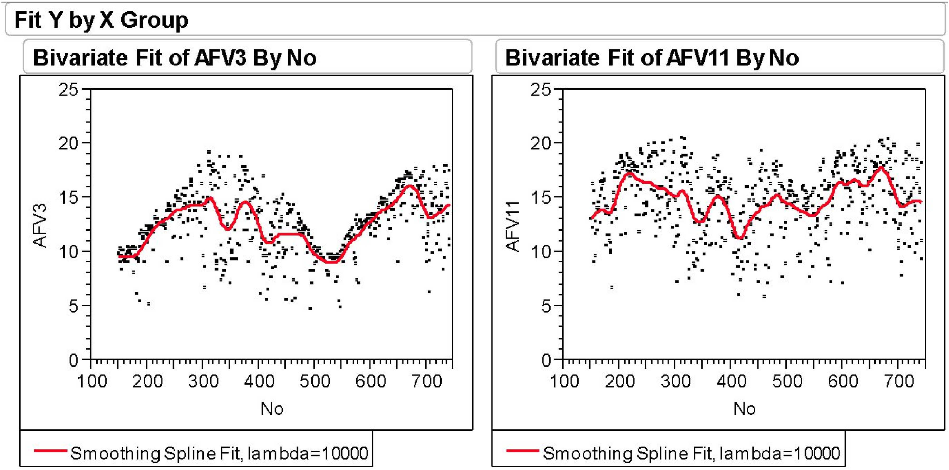
Individual generation of $A F V 3$ and $A F V 11$ .

Although photovoltaic systems are technically identical, various geographic and environmental factors influence their performance. We observe that the production of AFV3 is more uniform compared to that of AFV11, although the average energy generated by AFV3 (12,41 kWh) is lower than that of AFV11 (14,84 kWh), which represents a difference of 19,6%. Although AFV11 shows a greater dispersion in its production, both systems generally exhibit similar behavior, as shown in Figure 2. Regarding the estimated average solar hours, AFV11 has an average of 4,46 h, while AFV3 has 3,72 h.

To compare both generators, Figure 3 shows the R data points and their spline fit (Rs).

Figure 3.

Spline fit of Rs.

Figure 3 shows the spline fit that defines the observed trend in the R relationship. It is notable that the electrical generation behavior of the AFVs is similar from mid-spring to early autumn. However, outside of this period, AFV11 produces up to 40% more than AFV3. This indicates that the Álvaro Obregón delegation has more favorable environmental conditions for photovoltaic production.

3.2 TSCI adjustment

Table 1 shows the initial and optimized values of the proposed model.

These values represent the initial test values of the model variables, and their corresponding optimized values achieved through TSCI fitting.

In this stepwise analysis, the three studied effects T, S and C were successfully minimized as all 11 coefficients are included in this model. It is observed that $S S_{r e s} = 0.37866812$ is very close to zero, which indicates that the fitted Yadj model is very close to the Rs relationship, meaning that the model obtained accurately represents the behavior of the real measured values.

Figure 4 illustrates this small difference mentioned above. In the graph, the Rs curve represents the information obtained with the spline of the original data, while Yadj is the TSCI adjustment that gives us the approximation to reality. With the findings, it is expected that in the coming years the behavior will closely approach the form represented by the adjusted model. It is notable that in both curves the index is greater than 1.

Figure 4.

Fit TSCI.

On the other hand, the ANOVA confirms that the model is highly significant, with very high determination coefficients ( $R^{2} y R_{a d j}^{2}$ ). Table 2 shows the parameters obtained from the ANOVA.

Table 2.

ANOVA parameters.

Source	DF	SS	MS	F ratio	Prob > F	$R^{2}$	$R_{a d j}^{2}$
Model $y_{a d j}$	11	14,3133	1,30121	1999,9164	<<1e-100	0,97423	0,97379
$S S_{r e s}$	582	0,37867	0,00065
$C o r r T o t a l$	593	14,6919

From the previous table it is observed that the mean square of the residual (0,00065) is quite small compared to the mean square of the model (1,30121), making the Fratio statistic have a high value and its $P - v a l u e$ very small compared to a significance at 5%. These parameters validate the importance and precision of the three-effects model, highlighting its highly significant predictive capacity.

4. Conclusions

Due to the complexity inherent in accurately determining conditions affecting PV systems, such as microclimates and cloud cover, this study offers an approach based on three effects and statistical variability to improve the estimation of PV nominal power. It has been proven that the combination of third-degree Spline adjustment with smoothing and the TSCI technique, which separates the factors of trend, seasonality and the cyclical effect, with stepwise optimization, constitutes a reliable alternative in the energy analyzes of photovoltaic systems.

The R index simplifies the comparison of photovoltaic production in the places where AFV3 and AFV11 are installed, reaching values close to 1,5. This clearly demonstrates that the Álvaro Obregón Mayor's Office has greater solar generation potential. Thus, the installers will know that it will be necessary to project more nominal power in the La Magdalena Contreras Mayor's Office to generate the same energy as in the Álvaro Obregón delegation.

As future work, at least two photovoltaic systems will be analyzed in each mayor's office of Mexico City, of different typologies and installed powers, with the expectation of validating the presented methodology with greater efficiency and precision. In this way, a mapping will be obtained that will reduce the uncertainty in the quantification of the photovoltaic energy produced.

Footnotes

Acknowledgments

We would like to express our gratitude to LOGEN S.A de C.V. for providing the information necessary for the completion of this work.

Author contributions

This work introduces an innovative methodology that combines spline adjustment and the TSCI model to model the behavior of photovoltaic production in systems interconnected to the grid with a minimum of inputs, ignoring environmental variables. In addition, it offers the ability to identify the solar resource and determine the most conducive locations for the practical installation of solar arrays, thus benefiting users of this technology. Furthermore, this methodology is easily reproducible at any latitude.

Declaration of conflicting interests

The authors declared no potential conflicts of interest with respect to the research, authorship, and/or publication of this article.

Funding

The authors received no financial support for the research, authorship, and/or publication of this article.

ORCID iD

Raúl Alberto López-Meraz

Author Biographies

Raúl Alberto López-Meraz holds a PhD in Engineering and is a member of the National System of Researchers. His research focuses on the analysis and management of renewable energies in power grids, microgrids, and smart grids. Additionally, he explores topics such as the relationship between environmental variables and renewable energy generation, as well as sustainability aspects in the energy sector.

Ce Tochtli Méndez-Ramírez holds a PhD in Engineering and is a member of the National System of Researchers. His area of interest centers on the development of engineering solutions from a sustainability perspective.

Luis Omar Jamed-Boza holds a PhD in Mathematical Sciences with a specialization in Mathematical Statistics. His research lines focus on the application of statistical methods in the energy sector, with a particular emphasis on sustainability aspects.

References

Abril

(2011) Análisis de la evolución de las técnicas de series de tiempo. Un enfoque unificado. Estadística 63(181): 5–56. Instituto Interamericano de Estadística.

Araujo

Kitagawa

Weyll

, et al. (2023) Wind power forecasting in a semi-arid region based on machine learning error correction. Wind 3: 496–512.

Beveridge

Schechter

(1970) Optimization: Theory and Practice. New York: McGraw-Hill, pp. 124–140.

Bowman

Azzalini

(1997) Applied smoothing techniques for data analysis: The kernel approach with s-plus illustrations. In: Oxford Statistical Science Series, 18. Oxford: Clarendon Press, 193.

Chapra

Canale

(2021) Numerical Methods for Engineers. 8th ed. New York, USA: McGraw-Hill.

Couture

Beal

Antar

(1992) The Cubic Spline Interpolation of a Standing Wave Enve-Lope. Chicago, IL, USA: Antennas and Propagation Society International Symposium. AP-S.

Díaz-Araujo

Medina

Cisneros-Magaña

, et al. (2018) Periodic steady state assessment of microgrids with photovoltaic generation using limit cycle extrapolation and cubic splines. Energies 11: 2096.

Dudek

(2023) STD: A seasonal-trend-dispersion decomposition of time series. IEEE Transactions on Knowledge and Data Engineering 35(10): 10339–10350.

Fabara

Maldonado

Soria

, et al. (2019) Prediction of generation in a photovoltaic system through the application of data mining techniques. Revista Técnica “Energía” 16(I): 69–77.

10.

Gil

(2016) Pronóstico de la demanda mensual de electricidad con series de tiempo. Revista EIA 13(26): 111–120.

11.

Hopwood

Gunda

(2022) Generation of data-driven expected energy models for photovoltaic systems. Applied Sciences 12: 1872.

12.

IEA (2023) Tracking Clean Energy Progress 2023. Paris: IEA. Available at: https://www.iea.org/reports/tracking-clean-energy-progress-2023.

13.

IEA (2024) Renewables 2023. París: IEA. Available at: https://www.iea.org/reports/renewables-2023.

14.

JMP 8.0.2 (2009) SAS Institute Inc.

15.

Lindig

Louwen

Moser

, et al. (2020) Outdoor PV system monitoring—input data quality, data imputation and filtering approaches. Energies 13: 5099.

16.

López

Hernández

Jamed

, et al. (2020) Spline adjustment for modelling solar intermittences. Redin. Revista Facultad de Ingeniería. Universidad de Antioquía 94: 77–86.

17.

Petrinovic

(2008) Causal cubic splines: Formulations, interpolation properties and imple-mentations. IEEE Transactions on Signal Procesing 56: 5442–5453..

18.

Salinas

González

(2023) Modelo para la predicción de interrupciones de energía en circuitos de distribución reportados a la superintendencia de servicios públicos Colombia. [online]. Dsiponible en. Available at: http://hdl.handle.net/11371/6030.

19.

Terrerros

(2017) Nuevos modelos de predicción a corto plazo de la generación eléctrica en plantas basadas en energía solar fotovoltaica. Tesis doctoral, Universidad de la Rioja.

20.

Wolberg

Alfy

(1999) Monotonic cubic spline interpolation. Computer Graphics International, Proceedings. Canmore, Alta Canada.

21.

Lai

Bai

, et al. (2020) Optimal kernel ELM and variational mode decomposition for probabilistic PV power prediction. Energies 13: 3592.

22.

Yajure

(2023) Methodology based on data science for the development of a forecast of the power generation of a photovoltaic solar plant. Ingenius, Revista de ciencia y tecnología 30: 19–28.