Sage Journals: Discover world-class research

Abstract

Range prediction of electric vehicles requires knowledge of many parameters, including information about the vehicle environment. As an alternative to onboard measurement, external data sources (secondary data) can be used. The presented methods are suitable for estimating climatic data for vehicle application including urban areas and areas of complex topography. Compared to an inverse distance weighting approach for ambient temperature values, Kriging yields better overall accuracy especially for areas of complex topography, improving accuracy in urban regions, however, remains a challenge. An approach to improve accuracy in urban areas by considering local climate zones in the selection of secondary data sources produces mixed results.

Keywords

Local climate zones kriging naturalistic driving observation secondary data weather data

Introduction

Range anxiety and high vehicle costs are among the biggest hurdles to the spread of electric vehicles. By predicting the vehicle´s energy consumption for a route based on logged vehicle data, the remaining range can be determined. Range prediction can be performed using a machine learning approach or physical modelling, and the intended use case is usually prediction of the remaining range during the trip based on the planned route and trip history. Another application is the usage of logged data of a (to be electrified) driving profile for the identification of the optimal battery capacity to reduce investment costs.

The drivetrain usually accounts for the largest share of vehicle energy demand; however, total energy consumption also depends to a considerable extent on external influences, including not only traffic and route characteristics but also climate influences. For electric vehicles, the influence of climatic conditions on vehicle energy demand increases significantly compared to combustion vehicles since the total amount of energy available is lower while required heating can no longer be covered (predominantly) by waste heat from the drivetrain and must therefore be provided by the battery. Low ambient temperature is especially critical as depending on vehicle type and driving profile, range can be reduced to less than half on cold winter days,¹ whereby also minor temperature differences can have a noticeable effect on energy consumption and thus range.

Precise range prediction therefore requires detailed data on vehicle environment (slope, temperature, humidity and solar radiation). However, this information often cannot be recorded onboard with sufficient accuracy without additional equipment or – in case of predictions for upcoming tour segments – is not yet known. Instead, secondary data sources can be used, for climate data measurements and forecasts from weather services are suitable. Since these values are recorded at a different location and under different (non-road) conditions, the challenge lies in deriving the conditions at the vehicle. Hence despite the known importance climatic influences are often not or only loosely considered in range prediction.²

This paper presents methods for estimating climate conditions at vehicle route points at the current time, the past or the very near future based on meteorological measurements on the example of the ambient temperature. Information on the vehicle environment can also be used for applications beyond range prediction, e.g. warning of weather hazards.

Secondary data

Secondary data enrichment requires the location- and time-related estimation of the required values for each route point. If the tracks to be covered are in the future, data from weather forecast models can be used, for example the ICON model of the German Weather Service (DWD).³ Forecast data are available as a grid model with a grid size of a few kilometres and usually one value per hour for each size with a forecast period of up to ten days. By its nature, forecast values are subject to inaccuracies. If values are required for the current time or the past, measured values from weather stations can be used. For temperature values the German Weather Service provides measurement data from about 500 stations in Germany free of charge with a temporal resolution of 10 min. In many other countries, weather data is also available free of charge from the respective state weather service.

Value estimation for the vehicle is done by interpolation from the station measurements. The most commonly used spatial interpolation methods include

⁃ Nearest Neighbour method (NN), where the distance based nearest station is selected and its value adopted

⁃ Inverse Distance Weighting (IDW), where all surrounding sources are included in the calculation with an additional weight which decreases the influence of each source depending on distance

⁃ Kriging, where the weighting is based not only on distance but also on spatial structure

The Nearest Neighbour method only uses information from one source and direction, which can lead to high deviations if conditions at this source location differ from these at the vehicle location. Advantages of IDW and Kriging are that information from different sources and all directions is included. For vehicle application on ambient temperature estimation, IDW provides higher accuracy when compared to the NN method,⁴ but areas of complex topography showed increased deviations for both methods. The results of IDW in these areas can be improved by including altitude differences in station selection⁵ and thus only including stations at a comparable elevation to the vehicle in the calculation.

By taking the spatial structure into account, interpolation by Kriging instead of IDW offers further potential for improvement in this regard. For urban areas the climatic differences between the inner city and outer areas need to be considered. By applying local climate zones, the environment of vehicle and station can be classified, allowing only weather stations with similar climatic conditions to be included in the estimation.

Local climate zones

Climatic conditions in cities usually differ from those of their surrounding areas. The reasons for this are manifold,^6–8 but mainly due to buildings, surface sealing, heat influx and air pollution. Regarding the estimation of climatic values, measurements from the city surroundings are therefore only partially representative for the conditions in the city centre and vice versa. Thus, it may be beneficial for the estimation to be based on stations with environmental conditions similar to the vehicle surroundings only.

This approach requires information about the nearby environment of both locations. Steward and Oke⁹ developed a method to classify regions into a total of 17 categories based on development, vegetation and soil conditions (Figure 1), ten of them for urban (1–10) and seven for natural areas (A – G). A region can be divided into zones of e.g. 100 × 100 m and have their local climate zone (LCZ) classified. The approach is widely used in the field of urban climate research,^10–12 a grid model containing the classified land area of Europe in zones of 100 × 100 m is freely available.¹³

Figure 1.

Classification of local climate zones.⁹

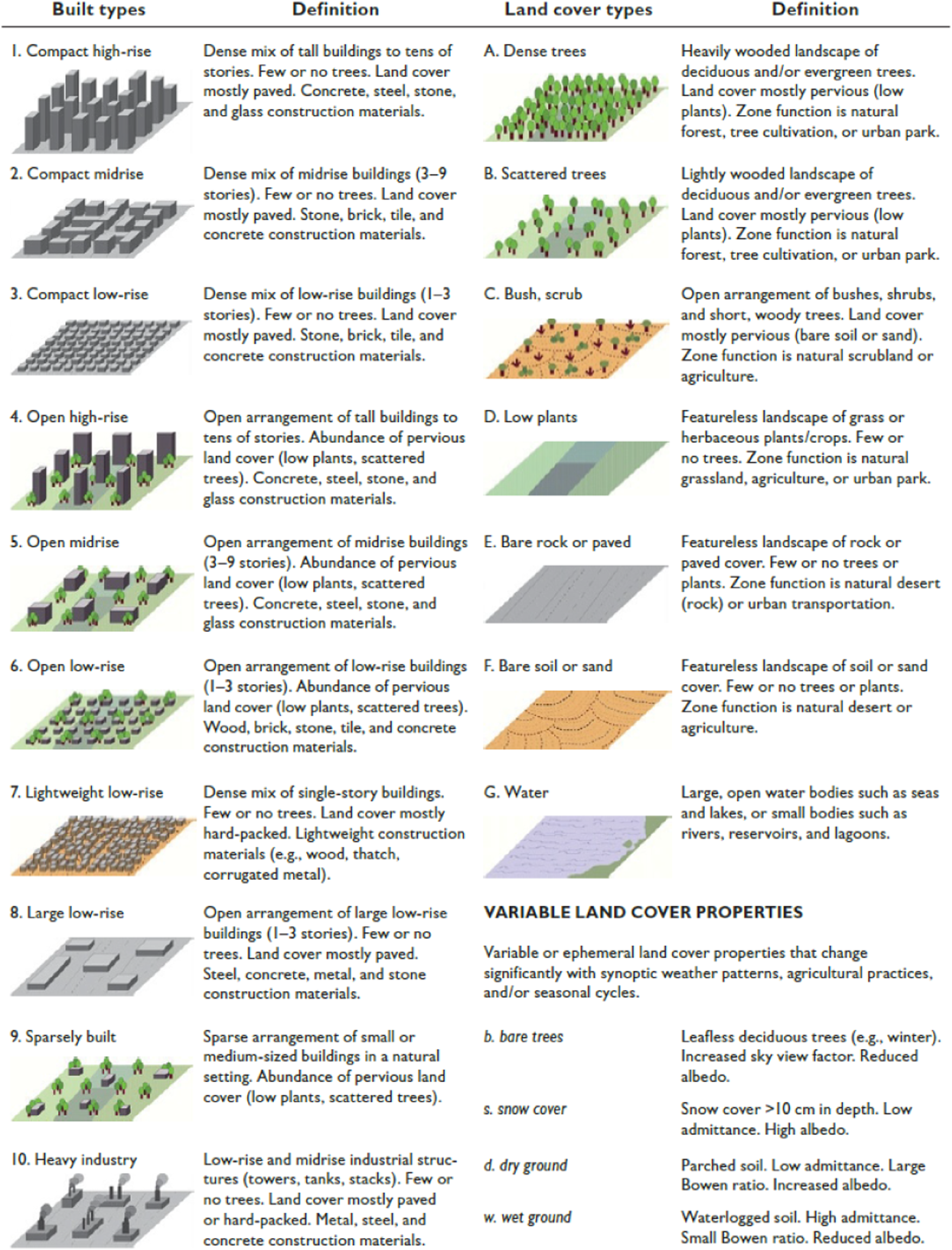
As climatic differences between two points tend to increase with distance, the selection of close weather stations remains important. Since the amount of weather stations in a region is limited, usually not every zone has a matching station in a region. A selection based purely on a zone identical to the vehicle location is therefore not advisable.

Studies of the temperature conditions of local climate zones in various cities show distinctive differences especially between urban and natural zones, whereby for the lightly populated zone 9 frequently conditions similar to those in neighbouring natural zones could be observed.^11,14 Therefore, two groups consisting of zones 9 and A to G as well as zones 1–8 and zone 10 are established and station selection is limited to stations of the same group.

IDW using local climate zones

For evaluation the method is applied for the estimation of ambient temperature values of a driving profile, as measured values of the temperature sensor on the vehicle are available for validation. Estimated values will then be compared to the measured values of the vehicle’s temperature sensor. The driving profile consists of logged data of a battery electric 18t commercial vehicle in everyday use in the area of Berlin and surroundings in logistics. The driving profile covers approx. 39.000 km over a continuous period of about 1.5 years in the years 2018–2020.

For spatial interpolation a refined IDW approach is used⁵ (equation (1)). This IDW approach takes altitudinal differences between vehicle and station into account, as the air temperature tends to decrease with increasing altitude. The term $z_{(x, y), h, t, q}$ represents the estimated temperature value at a (vehicle) location with coordinates x, y, altitude h, at time $t$ . Its value is calculated of the weighted average overall $n$ neighbouring stations with $z_{i, h, t}$ being the measured temperature from the ith station at time t, fitted to (vehicle) altitude h, $d_{i, (x, y)}$ the horizontal distance between the location $x, y$ and ith station, and the weighting factor $q$ . The distance weighting factor $q$ determines how strong the decrease of the influence of a value is with increasing distance.

z_{(x, y), h, t, q} = \frac{\sum_{i = 1}^{n} z_{i, h, t} d_{i, (x, y)}^{- q}}{\sum_{i = 1}^{n} d_{i, (x, y)}^{- q}}

(1)

The fitting to the vehicle altitude h is done by determining the difference in altitude

Δ h

between station and vehicle and applying a temperature lapse rate

Γ_{t}

(equation (2)). For the lapse rate

Γ_{t}

, a month-dependent value suitable for central Germany is used (Table 1).

z_{i, h, t} = z_{i, t} + Γ_{t} Δ h

(2)

Table 1.

Temperature lapse rate $Γ_{t}$ depending on month.⁶

Month	Jan	Feb	Mar	Apr	May	Jun
Γ_t (K/100 m)	0.39	0.56	0.61	0.67	0.67	0.64
Month	Jul	Aug	Sep	Oct	Nov	Dec
Γ_t (K/100 m)	0.65	0.63	0.57	0.55	0.49	0.50

The method also includes an exclusion of stations when altitude differences from the vehicle are too high, but since only small altitude differences occur in the Berlin/Brandenburg region, this approach is not applied. The method is also compared with the results of an IDW without consideration of LCZ in the station selection. The estimation was done for both approaches using the same parameters with a weighting factor of q = 1, which was identified as optimal for this region.

Table 2 contains the deviations between estimated and vehicle sensor value for all valid points of the data set. When comparing the IDW results, a clear improvement of all criteria can be seen by including the local climate zone in the stations selection (IDW_LCZ), resulting in a MAE reduction of 0.16°C or 8.6%. However, with an MAE of 1.69°C between sensor and estimate, there is still a significant deviation from the sensor values of the vehicle. The positive mean value for both methods shows a clear trend towards underestimation of the ambient temperature measured by the vehicle’s sensor. A tendency of vehicle sensors to measure higher temperature values when compared to stationary measurements was also found in investigations of other authors,^15,16 a probable explanation for this is the influence of vehicle waste heat on the measurement. Since the investigated vehicle is electric driven, the influence is less strong in this case.

Table 2.

Overall temperature deviation (sensor value – est. value) of the selected driving profile.

Method	Mean [°C]	MAE [°C]	RMSE [°C]
IDW-LCZ	1.65	1.69	2.04
IDW	1.83	1.85	2.19

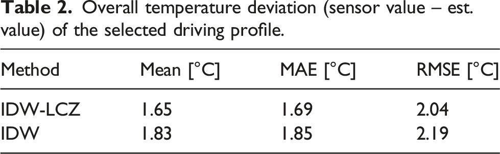
Figure 2 shows the mean absolute deviation of both methods depending on the local climate zone of the driving profile’s measuring points. As can be seen from the probability density, the vehicle was mainly in use in zones 6, 8 and D. For some zones, no values are available because the vehicle was not in such a zone at any time during data logging. For nearly all remaining zones, an accuracy increase could be achieved by including local climate zones. However, the gains are smaller for natural zones (A–D) where in some cases no improvement or even minimal deterioration was achieved.

Figure 2.

Overall temperature deviation (sensor value – est. value) by local climate zone.

The accuracy improvement in naturalistic zones is due to the fact that the driving profile covers areas of Berlin’s near surroundings, so when LCZs are considered, inner city stations are no longer included in the value estimation. Thus, areas far from bigger cities are expected to have smaller or no improvements.

To eliminate the possible influence of vehicle waste heat on the result, the method was additionally examined on the basis of the measured weather station values with the use of cross-validation (leave-one-out). For this purpose, one station is removed from the station network at a time and a value is estimated for each measurement of the removed station based on the remaining stations, the error of the method is then determined by comparison with the real measurement. Since improvements by integration of local climate zones can only be expected in the vicinity of large cities, the Berlin–Brandenburg region (approx. 30.000 km²) was selected. The cross-validation includes all valid hourly DWD measurements of this region (29 weather stations) in 2020. The results were compared with the IDW which was performed with the same data set (Table 3).

Table 3.

Results for cross-validation of DWD temperature measurements for Berlin and Brandenburg.

Method	Mean [°C]	MAE [°C]	RMSE [°C]
IDW-LCZ	0.10	0.64	0.96
IDW	0.04	0.60	0.90

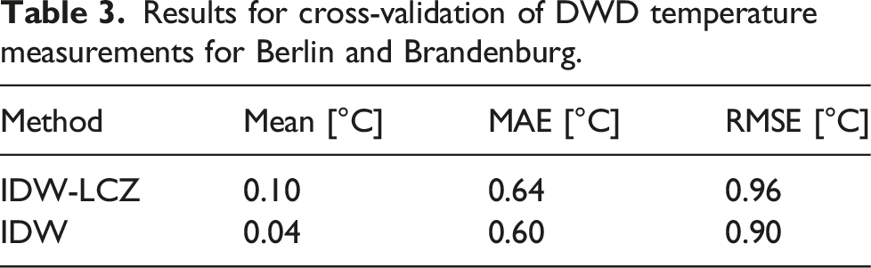
In the cross-validation, the integration of LCZ shows a slight increase in the resulting error. Although only stations with a similar climatic environment are now considered, this also increases the (average) distance of the selected stations, which can in turn increase the error. In addition, the investigated area now covers more rural regions away from large cities, where no improvement can be expected by using local climate zones. Considering only the city area of Berlin is not reasonable, as only five stations are active there – and thus only five unique locations could be examined.

The results are in contrast to those of the driving profile, where a higher accuracy was observed. Investigations of other driving profiles in the Berlin Brandenburg region also showed improvements through use of local climate zones, albeit to a lesser extent. Due to the influence of waste heat on the sensor measurement, an evaluation of the real accuracy gain is difficult, since the real ambient conditions are not exactly known. As natural zones tend to be cooler than urban ones, considering LCZ in an urban area therefore means that neighbouring natural stations are no longer considered and thus the estimated temperature at this position increases, which reduces the error to the (inflated) sensor value and vice versa. In natural zones, however, an increase in deviation would then have to be expected, but the results for the driving profile also show a (slight) improvement there. In conjunction with the cross-validation results it appears that the benefits are dependent on location and cannot be generalized. The zones used are quite small (100 × 100 m), due to this the surroundings of station and vehicle may not always be well represented. For example, weather stations at airports are often assigned to the natural space due to the lawn. Steward and Oke⁹ point out that a zone diameter of 400–1000 m is necessary for the air masses to adequately adapt to the surface. Investigations with larger zones by combining adjacent zones (to a zone up to 10 × 10 km) showed slight improvements, but again no overall better accuracy could be achieved.

Kriging of weather data

With Kriging, similar to the IDW, locations with a shorter distance to the target location are weighted higher than locations further away. The crucial difference between these two methods is the determination of these weights. While in the classical IDW the weighting is determined only by the distance itself and some freely selectable parameters, the spatial distribution structure of the observed variable is used for the interpolation in the kriging methods.¹⁷ It determines thereby substantially the actual weighting of individual neighbouring locations. This calculation is done in accordance with probability theory, so that in distinction to IDW the kriging methods are also called statistical interpolation methods, see.¹⁸ In order to include the spatial structure of a variable in its interpolation, the so-called variogram is often used in kriging. The variogram results from the consideration of the variances of all location pairs of a sample data set and provides, among other things, information about the spatial dependence of the measured variable.^19,20

There are several approaches to kriging: simple, ordinary and universal kriging.²¹ In principle, it can be stated that a variable with a (spatially) known and constant mean favours simple kriging, a constant but unknown mean favours ordinary kriging, and an unknown and deterministically variable mean favours universal kriging (UK), see Ref.[21]. If the correlation between the examined variable and other variables is known, the use of cokriging, a multivariate extension of the univariate kriging methods, should be considered too, see.¹⁷ Thus, before creating a variogram, it should be investigated whether the mean, and consequently the variable itself, is subject to spatial trends and, furthermore, whether it is directly related to other variables. With respect to air temperature, a distinctive trend with increasing measurement altitude could be found for the area of Germany in particular. A suitable auxiliary data set could not be created so far, so that univariate universal kriging was selected as an interpolation method.

Accuracy is again checked by cross-validation based on almost all valid hourly temperature measurements of the German Weather Service for the year 2020 (except mountain stations Zugspitze and Feldberg), the results were again compared with the IDW which was performed with the same data set.

As Table 4 shows, significant improvements in interpolation accuracy were achieved compared to the IDW method. For the RMSE and MAE, general reductions of 6.93% and 5.65%, respectively, were achieved. The differences between the two interpolation approaches are plotted in Figure 3, where locations with improvements over IDW are marked in green and deteriorations in red; the diameter of the dot additionally indicates the absolute difference of the Kriging method over IDW. Improvements compared to the adjusted IDW were primarily achieved in regions with complex topography, such as in central or southern Germany. General improvements of the RMSE value are especially noticeable for low mountain ranges like the eastern Bavarian Forest, the Franconian Alb or the Thuringian Forest. Further improvements of the interpolation precision can also be seen in coastal regions. Increased RMSE values of the universal kriging compared to the IDW do not seem to occur systematically. It is therefore assumed that the applied universal kriging has a higher suitability for the interpolation of air temperatures.

Table 4.

Results for the cross-validation of DWD temperature measurements.

Method	Mean [°C]	MAE [°C]	RMSE [°C]
UK	−0.0027	0.7179	0.9765
IDW	−0.0024	0.7609	1.0493

Figure 3.

Differences of the RMSE between UK and IDW for Germany (Map ©^22,23).

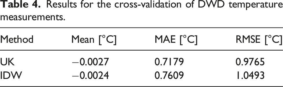
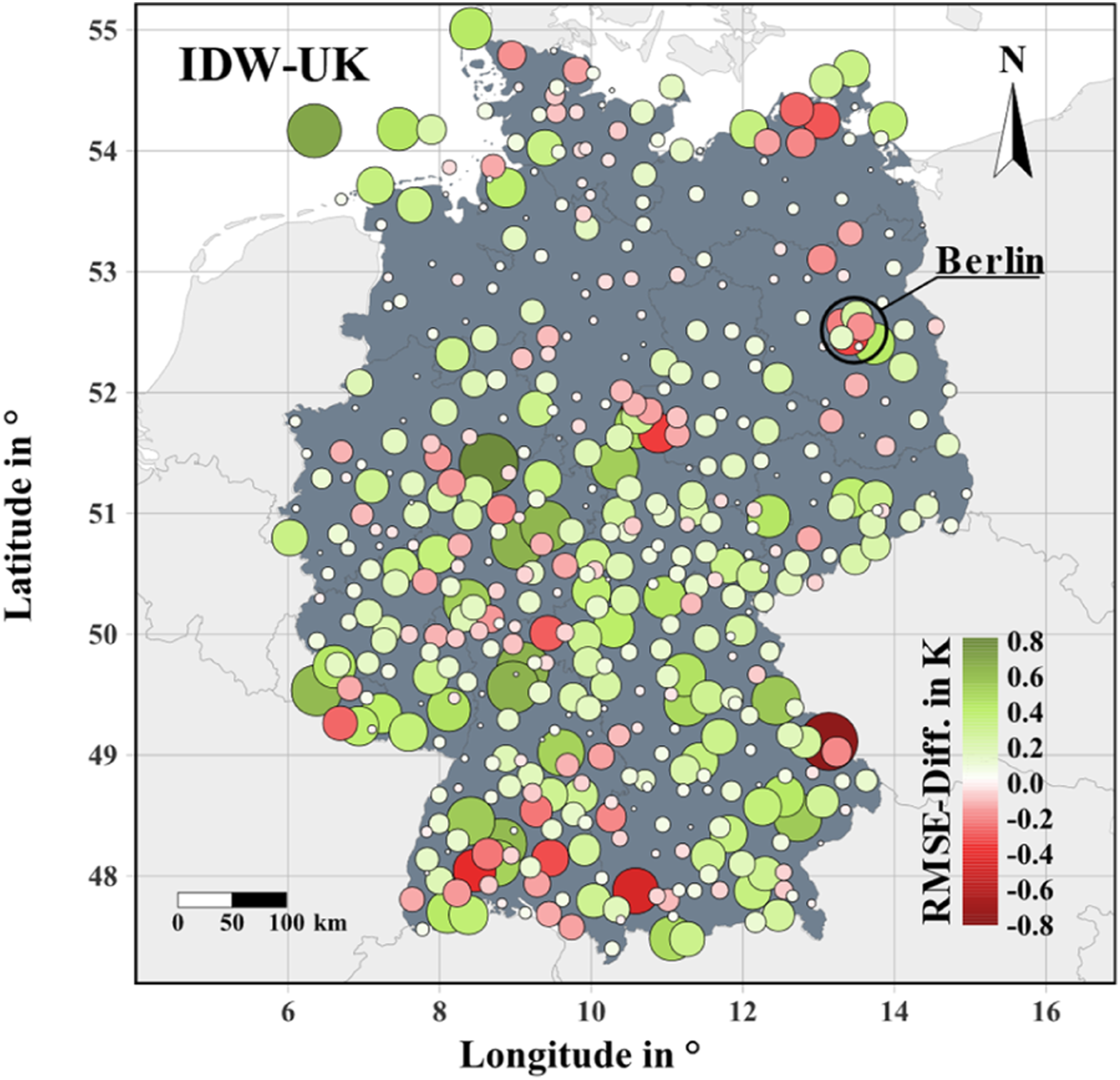
However, potential challenges of the presented UK-based approach became apparent especially in urban regions, see Berlin in Figure 3, were no improvement over IDW could be achieved.

Conclusion

In this paper, methods for weather data enrichment focused on automotive application were examined. The methods presented were shown for the estimation of ambient temperature values but are also suitable for other influencing variables such as humidity. The goal was to improve upon basic approaches such as IDW.

A switch from IDW to Kriging interpolation was established, yielding a MAE reduction of 0.05°C or 5.65% over the whole station network of Germany for a period of one year. For Kriging, improvements in areas of complex topography can be seen, but prediction for urban areas remains a challenge. For improvements in urban zones, the integration of local climate zones into IDW was examined, but no general improvement could be achieved. The evaluation of LCZ was complicated by the fact that the measurement values at the vehicle are biased due to waste heat, while in cross-validation only a few locations can be tested since weather stations are mostly sited in non-urban areas. The distortion due to waste heat further emphasizes the need to use secondary data to obtain accurate information about the vehicle’s ambient climatic conditions.

The next step is to combine local climate zones and kriging, as kriging offers potential for better utilization of LCZs by analysing spatial structure. For this, local climate zones have to be included as an additional variable, requiring a cokriging approach. Therefore, the local climate zones must be provided in numerical form instead of classes, a numerical ranking of these very zones has therefore to be established. Cokriging also allows the addition of further influences as additional variables. For the consideration of topographical influences, the geographical altitude can be investigated as an additional variable.

Footnotes

Declaration of conflicting interests

The author(s) declared no potential conflicts of interest with respect to the research, authorship, and/or publication of this article.

Funding

The author(s) disclosed receipt of the following financial support for the research, authorship, and/or publication of this article: We acknowledge support by the German Research Foundation and the Open Access Publication Fund of TU Berlin.

ORCID iDs

Thomas Herzlieb

Johannes H. L. Sturm

References

Delos Reyes

JRM

Parsons

Hoemsen

. Winter Happens: The effect of ambient temperature on the travel range of electric vehicles. IEEE Trans. Veh. Technol 2016; 65: 4016–4022, doi:10.1109/TVT.2016.2544178

Liu

Wang

Yamamoto

, et al. Exploring the interactive effects of ambient temperature and vehicle auxiliary loads on electric vehicle energy consumption. Applied Energy 2018; 227: 324–331.

Wetterdienst

. Numerical weather prediction models - ICON (icosahedral nonhydrostatic) model, 2022, https://www.dwd.de/EN/research/weatherforecasting/num_modelling/01_num_weather_prediction_modells/icon_description.html?nn=484268 (accessed 2 February 2022).

Jerratsch

J-O

Herzlieb

Marker

. Using secondary data to reduce measuring efforts in naturalistic driving observation: for energetic simulations and EV-optimization. In: Technische Universität München and Bayern InnovativConference on future automotive technologies: CoFAT 2018, Germany, 2018.

Jerratsch

J-O

Herzlieb

Marker

. Weather data mapping to enrich naturalistic driving data and enhance energetic simulation. In: FISITA 2018 World Automotive Congress Proceedings: Disruptive Technologies for Affordable and Sustainable Mobility, Chennai, 2018.

Hupfer

Kuttler

(eds). Witterung und Klima: Eine Einführung in die Meteorologie und Klimatologie. 10., völlig neubearbeitete Auflage. Wiesbaden: Vieweg+Teubner Verlag, 1998.

Malberg

. Meteorologie und Klimatologie: eine Einführung ; mit 56 Tabellen. 5., erw. und aktualisierte Aufl. Berlin: Springer, 2007.

Mühlbacher

Koßmann

Sedlmeier

. Stadtklimatische Untersuchungen der sommerlichen Temperaturverhältnisse und des Tagesgangs des Regionalwindes (Alpines Pumpen) in München. Berichte des Deutschen Wetterdienstes. Offenbach am Main: Selbstverlag des Deutschen Wetterdienstes, 2020, 252.

Stewart

Oke

. Local climate zones for urban temperature studies. Bulletin of the American Meteorological Society 2012; 93: 1879–1900.

10.

Stewart

Oke

Krayenhoff

. Evaluation of the ‘local climate zone’ scheme using temperature observations and model simulations. Int. J. Climatol 2014; 34: 1062–1080.

11.

Skarbit

Stewart

Unger

, et al. Employing an urban meteorological network to monitor air temperature conditions in the ‘local climate zones’ of Szeged, Hungary. Int. J. Climatol 2017; 37: 582–596.

12.

Verdonck

M-L

Demuzere

Hooyberghs

, et al. The potential of local climate zones maps as a heat stress assessment tool, supported by simulated air temperature data. Landscape and Urban Planning 2018; 178: 183–197.

13.

Demuzere

Bechtel

Middel

, et al. Mapping Europe into local climate zones. PloS One 2019; 14: e0214474.

14.

Stewart

Oke

. Thermal differentiation of local climate zones using temperature observations from urban and rural field sites. In: Ninth Symposium on Urban Environment, American Meteorological Society, Keystone, 2010.

15.

Hellweg

Nachtigall

Kratzsch

, et al. Fleet weather map - a project to integrate floating car weather data into the field of automated driving, 2019. In: Transportation Association of Canada and ITS Canada 2019 Joint Conference and Exhibition, Canada, 2018. https://trid.trb.org/view/1682683

16.

Rietdorf

Kratzsch

Nachtigall

, et al. Korrekturansätze für Fahrzeugsensordaten zur realen Erfassung des Straßenwetters. ATZ Automobiltech Z 2021; 123: 66–70.

17.

Webster

Oliver

. Geostatistics for environmental scientists. Chichester: Wiley, 2001.

18.

Hengl

. A practical guide to geostatistical mapping of environmental variables. Luxembourg: Publications Office, 2007.

19.

Burger

Skala

. Die Untersuchung ortsabhängiger Variablen: Modelle, Methoden und Probleme. Geol Rundsch 1978; 67: 823–839.

20.

Mesić Kiš

. Comparison of ordinary and universal kriging interpolation techniques on a depth variable (a case of linear spatial trend), case study of the Šandrovac field. Rudarsko Geolosko Naftni Zbornik 2016; 31: 41–58, https://www.researchgate.net/publication/301788692_Comparison_of_Ordinary_and_Universal_Kriging_interpolation_techniques_on_a_depth_variable_a_case_of_linear_spatial_trend_case_study_of_the_Sandrovac_Field

21.

Wackernagel

. Multivariate geostatistics. Berlin, Heidelberg: Springer Berlin Heidelberg, 2003.

22.

Hijmans

. DIVA-GIS, 2021, https://www.diva-gis.org/gdata.

23.

Earth Natural . Free vector and raster map data at 1:10m, 1:50m, and 1:110m scales, 2021, https://www.naturalearthdata.com/downloads/10m-cultural-vectors/10m-admin-0-countries/ (accessed 13 May 2022).

Kriging and local climate zones – key to higher accuracy in range prediction?

Abstract

Keywords

Introduction

Secondary data

Local climate zones

IDW using local climate zones

Kriging of weather data

Conclusion

Footnotes

Declaration of conflicting interests

Funding

ORCID iDs

References