Sage Journals: Discover world-class research

Abstract

Glass fiber-reinforced plastics (GFRP) is widely used in many industrial fields. When acoustic emission (AE) technology is applied for dynamic monitoring, the interfering signals often affect the damage evaluation results, which significantly influences industrial production safety. In this work, an effective intelligent recognition method for AE signals from the GFRP damage is proposed. Firstly, the wavelet packet analysis method is used to study the characteristic difference in frequency domain between the interfering and AE signals, which can be characterized by feature vector. Then, the model of back-propagation neural network (BPNN) is constructed. The number of nodes in the input layer is determined according to the feature vector, and the feature vectors from different types of signals are input into the BPNN for training. Finally, the wavelet packet feature vectors of the signals collected from the experiment are input into the trained BPNN for intelligent recognition. The accuracy rate of the proposed method reaches to 97.5%, which implies that the proposed method can be used for dynamic and accurate monitoring of GFRP structures.

Keywords

glass fiber-reinforced plastics acoustic emission wavelet packet analysis back-propagation neural network intelligent recognition

Introduction

Glass fiber-reinforced plastics (GFRP) is a type of multiphase solid composite made from glass fibers and synthetic resins. The GFRP exhibits excellent resistance to fatigue, electrical and thermal load, and corrosion.^1,2 In the last several decades, the GFRP has been widely used in many industrial fields, such as aerospace, petroleum, transportation, and construction, due to the low production cost and good material properties.^3
–5 For these applications, the progressive damage during manufacturing and service has led to a significant failure of GFRP structures and caused serious security accidents.^6
–8

Acoustic emission (AE) technology is a passive, real-time, and dynamic detection method. The collected signals come from the damage of the material.⁹ The AE source releases the elastic waves that can carry the damaged information of the tested material, and the collected signals can be recorded and analyzed with professional instruments. The method is suitable for the in-service security monitoring of GFRP.^10,11 Currently, numerous research studies have been conducted in the signal characteristics analysis and signal processing, damage mechanism identification, positioning and quantitative evaluation. By performing double-cantilever tests, Sause et al. found that the accumulative amplitudes of AE signals resulting from the interlaminal cracks were closely related to the composite mechanical properties. The evolved damage could be properly identified in combination with fractographical characterization.¹² After repeated impacts, Balan et al. examined the residual strength of unidirectional GFRP laminates at ambient and elevated temperatures by monitoring the evolved peak frequencies in three-point bending tests.¹³ Qi et al. proposed a focusing enhancement technique with virtual loading based on time-reversal theory to apply to AE source location for GFRP. The experimental results showed that the technique had positioning accuracy within 4% after the vibration amplitude of each pixel in the monitoring area was calculated and fluctuation image was reconstructed, which can meet the requirements of engineering applications.¹⁴ However, during the course of in-service security monitoring, it is found that there is strong environmental noise interference in the signals collected by the sensors, which significantly impact the damage identification and evaluation. On the one hand, the threshold value of the monitoring instrument is set higher that causes the weak AE signals to be ignored and results in missed detection. Moreover, when the strong interference exceeds the threshold value, it is considered as the damage signal, leading to misjudgment. Therefore, it is necessary to analyze the characteristics of the monitoring signals and distinguish the effective AE signals from the interfering signals. Then, the interfering signals can be removed and the effective AE signals can be retained for postprocessing and analysis to ensure the GFRP structure security.

In practical engineering applications, the wavelet analysis is an effective method for processing sudden and unstable signals. The wavelet packet analysis is a further optimized and improved version of the wavelet analysis.¹⁵ Bianchi et al. proposed an analyzing method for the extraction of single events in rail contact fatigue test based on a wavelet packet decomposition within the framework of multiresolution analysis theory and used the method to identify the parts of the recorded AE signals that belonged to different events and discern them from noise.¹⁶ In this study, the wavelet packet analysis was applied to process the AE signals, and the collected signal was decomposed into multiple two-dimensional parameters (time and position) and frequency to achieve the characteristic decomposition for the signals in different frequency bands and different times. The wavelet packet analysis has a strong time–frequency localized decomposition ability, which can provide reliable references for the extraction and recognition of signal types.¹⁷

The pattern recognition method is to train the signal recognition model by learning the historical data and then combine with real-time testing data to achieve accurate recognition and evaluation of the collected signals. Caggiano and Nele applied a multiple sensor system to develop an artificial neural network-based cognitive paradigm to predict tool wear. Selected statistical features extracted from the multiple sensor signals in the time domain were combined via sensor fusion techniques to construct sensor fusion pattern vectors. These were then fed to artificial neural networks for pattern recognition, with the goal of finding correlations that would allow the prediction of the corresponding tool wear, which could be utilized to support decision making at the appropriate time for worn tool replacement.¹⁸ Wang et al. investigated a smart process monitoring approach that employs (AE) to characterize the variations in the natural fiber-reinforced polymer machining process. The two types of the bidirectional-gated recurrent deep learning neural network (BD-GRNN) models were developed to predict the process conditions based on dynamic AE patterns. The results from the experimental study suggested that BD-GRNNs can correctly predict (around 87% accuracy) the cutting conditions.¹⁹ For AE monitoring of composites, to investigate the aging effect of GFRP exposed to seawater environment for different periods of time, Suresh Kumar et al. examined the mass gain ratio and flexural strength of GFRP laminates according to the changes in AE signal parameters for various periods of time after the seawater treatment. The significant AE parameters were considered as input data, which were taken from 40–70% of failure loads for developing the radial basis function NN and generalized regression neural network (GRNN) models, which both were able to predict the ultimate failure strength.²⁰ Sause et al. proposed an AE-based approach be able to use a combination of an artificial neural network to predict the materials present stress exposure and a simple linear extrapolation and predicted the failure strength within the margin of prediction error for all test cases studied, which could be used for the design and quality control of fiber-reinforced structures.²¹ Brunner discussed and classified the single dominant damage mechanism of fiber-reinforced polymer composites. Some approaches (e.g. pattern recognition or NNs) were introduced to identify the different microscopic damage mechanisms from AE signals obtained from various load tests.²² To identify damage modes exhibited in the GFRP coupons and composite systems with similar configurations, Nair et al. applied the unsupervised k-means clustering analysis to separate the AE date into several clusters and correlate each cluster to its corresponding failure mechanisms. After a reliable AE database was built for a typical sample of each test set, NNs based on multilayer perceptron and support vector machine algorithms were developed. The trained NNs were used to successfully identify damage modes in failure mechanism of CFRP-retrofitted reinforcement concrete beams and GFRP.^23,24 The above research work focused on the effective AE signal processing and analysis, but in the actual process of AE testing, interference signals often mixed in. If it could not be accurately identified, it would greatly affect the identification and evaluation for AE sources. Therefore, it was important to identify effective AE signals and remove interfering signals before the collected signals were further analyzed.

The back-propagation neural network (BPNN) is currently the most widely used machine learning method. Essentially, the back-propagation algorithm takes the square of the network error as the objective function and uses the gradient descent method to calculate the minimum value of the objective function. It has a strong self-adaptive ability and better fault tolerance. The BPNN can not only learn adaptively but can also adjust the size of the network adaptively.²⁵ Wu et al. proposed a fault diagnosis method based on BPNN for the grid-connected solar photovoltaic system. The experimental results showed that this method was efficacious and earthly.²⁶ In program debugging, Eric and Qi proposed the use of a BPNN, which had been successfully applied to software risk analysis, cost prediction, and reliability estimation, to help programmers effectively locate program faults. The results suggested that a BPNN-based fault localization method can be effective in locating program faults.²⁷

In this study, the intelligent recognition method based on wavelet packet decomposition and BPNN is carried out to achieve accurate recognition of the effective AE signals. The wavelet packet analysis method is used to extract the feature vectors of the two types of signals according to the frequency-domain difference between the interfering signal and the effective AE signal, which can effectively characterize the frequency band characteristics of the two types of signals. The collected signals are classified to accurately determine and distinguish between the effective AE signal and the interfering signal with the BPNN.

Recognition principle

Wavelet packet analysis principle

Wavelet analysis is a time-frequency localized analysis method with a fixed window area, whose shape can be changed, that is, both the time and the frequency windows can be changed. Since it only decomposes the low-frequency components and ignores the high-frequency components during the process of signal decomposition, its frequency resolution decreases with the increase in the frequency. The wavelet packet analysis developed based on the wavelet analysis is a more refined analysis method for signals. The wavelet packet analysis divides the time–frequency plane more finely and has higher resolution of the high-frequency components of the signal than that of the dyadic wavelet transform. Moreover, the wavelet packet analysis introduces the concept of optimal basis selection, that is, after the frequency band is divided into multiple layers, the optimal basis function can be adaptively selected to match the signal according to the characteristics of the analyzed signal that improves the signal analysis capabilities. Therefore, the wavelet packet analysis has a wide application range. From the view of signal processing, it allows the signal to pass through a series of filters with different center frequencies but the same bandwidth. It has the characteristics of time–frequency localization and it can better reflect the characteristics of the signal for analyzing the AE signal. The feature vector can adaptively select the frequency band. The features correspond to the frequency spectrum and improve the time–frequency resolution.²⁸

The structure of a wavelet packet decomposition tree is shown in Figure 1. The left and right nodes of each subtree represent the low-frequency and the high-frequency components of the decomposed signal, respectively, while S ₀₀ represents the original signal that is not decomposed. The decomposed components have the relationship shown in equation (1)

\begin{array}{l} S_{00} = S_{10} + S_{11} = S_{20} + S_{21} + S_{22} + S_{23} \\ \begin{matrix}  \end{matrix} \begin{matrix} = S_{30} + S_{31} + S_{32} + S_{33} + S_{34} + S_{35} + S_{36} + S_{37} \end{matrix} \end{array}

where S_ij represents the reconstructed signal at the j’th node in the i’th layer. For example, S ₃₅ is the reconstructed signal at the fifth node in the third layer. It can be seen that based on wavelet analysis, the decomposition of the high-frequency band which is not decomposed in the wavelet analysis is further refined to ensure that the decomposition has the same high-frequency resolution in the entire frequency domain.

Figure 1.

Diagram of three-layer wavelet packet decomposition tree.

After the signal is decomposed into i layer using the wavelet packet, there will be 2 ⁱ wavelet packet components. Each component matches a certain frequency band of the signal. Thus, the original signal can be recovered by the reconstruction algorithm.

The wavelet basis is an important part of the wavelet packet transform. A suitable wavelet basis is beneficial to accurately extract the characteristics of the signal. The wavelet basis that are applied to AE signals include Daubechies wavelet basis, Symlet wavelet basis, and Coiflet wavelet basis. In this study, the Daubechies wavelet basis is used to perform the wavelet packet transformation on the AE signals, and the correlation coefficient is used as the selection criterion to measure the signal approximation ability. When the vanishing moment N of the Daubechies wavelet basis is 4, the decomposition characteristics have a good correlation with the signal. The Db4 wavelet basis is selected to decompose the received AE signal into five layers in this study.

Parseval theorem can be expressed in equation (2)

\int_{- \infty}^{\infty} x^{2} (t) d t = \int_{- \infty}^{\infty} X (f) d f

The theorem shows that the total energy of the signal in the time domain is equal to that in the frequency domain. The wavelet packet energy is used to extract the received AE signal characteristics using the energy characterization.^29,30

After the wavelet packet decomposes the signal into the i’th layer, the frequency band energy of each component is calculated using equation (3)

E_{i j} = \int {|S_{i j} (t)|}^{2} d t = \sum_{k = 1}^{n} {|x_{i j} (k)|}^{2}

where S_ij is the j’th reconstructed signal in the i’th layer, and x_ij (k) is a discrete signal of S_ij with a signal length of n, and E_ij is the energy corresponding to the j’th reconstructed signal in the i’th layer. Then, the feature vector C of the received AE signal is calculated according to the following equations (4) and (5)

C = [c_{1}, c_{2}, \dots, c_{2^{i}}] = [\frac{E_{i 0}}{E}, \frac{E_{i 1}}{E}, \dots, \frac{E_{i (2^{i} - 1)}}{E}]

E = \sum_{j = 0}^{2^{i} - 1} E_{i j}

where E is the total energy of the signal. Each feature vector contains 2 ⁱ feature values. The different signal characteristics can be described and characterized by feature vector C.

Back-propagation neural network

The concept of BPNN was proposed by Rumelhart and McClelland in 1986. It is a multilayer feed-forward NN trained by the error back-propagation algorithm, which is mainly used in pattern recognition, prediction, and evaluation.³¹ To realize the accurate recognition for the AE signal from the damage in the GFRP, a three-layer BPNN model is applied to classify the signals through the wavelet packet feature vector.

The BPNN is composed of an input layer, several intermediate layers (hidden layers), and an output layer. The three-layer network can complete the nonlinear mapping from the input layer to the output layer. Figure 2 shows a three-layer topology structure of BPNN. There are multiple neurons operating at the same time in each layer. Each layer is connected with the lower layer for transferring information. However, there is no connection between the neurons in each layer.

Figure 2.

Topology structure of BPNN. BPNN: back-propagation neural network.

The training processes of BPNN include forward propagation and error back-propagation. During the forward propagation, the network model acts on the input layer. The output values of the neurons are calculated and transmitted to the output layer after processed by the hidden layer. During the error back-propagation, the output error (the difference between the expected and the actual output) is calculated while back-propagating along the original path to the hidden layer until the input layer. The error signal of each unit in each layer can be obtained by distributing the errors to each unit of each layer, which is the basis for correcting the weight of each unit. This calculation process is completed with the gradient descent method, and the weights of the neurons in each layer are constantly adjusted. The training process continues until the error is lower than the preset threshold. Therefore, the BPNN has the characteristics of automatic learning, self-adjustment, and hierarchical expression.³² The establishment process of the BPNN model is as follows.

Step 1. The number of nodes in each layer of BPNN

(1) The number of nodes in the input layer

The number of nodes in the input layer is determined by the dimension of the input feature vector. The feature vector should describe the characteristics of the collected signal. If the number of nodes is too large, the operation amount will increase. If the number of nodes is too small, it will not reflect the signal characteristics. In this study, two types of signals are decomposed using wavelet packet and feature vector containing 32 feature values is obtained. The feature vector is the input vector of the BPNN. Thus, the number of nodes in the input layer is 32.

(2) The number of nodes in the output layer

The AE and the interfering signals are effectively recognized and the expected output categories are AE signals “1” and interfering signals “0.” Thus, only two output results are needed and the number of nodes in the output layer is 2.

(3) The number of nodes in the hidden layer

A three-layer BPNN is adopted in this study, that is, there is only one hidden layer to realize the mapping relationship. In this work, the number of nodes in the hidden layer is selected according to the empirical equation (6)

p = \sqrt{j + q} + a

where, p, j, and q are the numbers of nodes in the hidden, the input, and the output layers, respectively, and 1 < a < 10. Therefore, the range of the number of nodes in the hidden layer is [6, 15]. Several calculating results with a different number of nodes in the hidden layer were compared and the minimum error was obtained with eight nodes. Thus, the number of nodes in the hidden layer of the BPNN is set to 8.

Step 2. Determination of transfer function

Transfer function is an important part of BPNN. The BPNN usually adopts continuous differentiable sigmoid function, which is soft and smooth and has better fault tolerance. The sigmoid function is divided into log-sigmoid and tan-sigmoid. The former has a range of (0,1), while the latter has a range of (−1,1). To ensure that the network output is limited to [0, 1], which is convenient for comparing the network output result with the target output, the log-sigmoid function is used as the transfer function of the hidden and the output layers.

Step 3. Initial weight selection

The initial weight is the determinant of the convergence speed and complexity in BPNN training. Since the transfer function is a log-sigmoid function, the initial weight is a random number from 0 to 1. In this study, the weight is randomly generated after the sample is input.

Step 4. The selection of learning rate, number of cycles, and expected error

The learning rate affects the change of BPNN weight in each iteration training cycle as well as the time and the convergence speed of BPNN training. Generally, the learning rate is between 0.01 and 1 in the classification recognition. In this study, the learning rate is set to 0.1. The expected error of BPNN training is 0.01, and the maximum iteration number is 1000.

Experimental testing and analysis

Specimen preparation

The GFRP specimens were made from No. 430 resin and woven glass fiber. The cross plies were placed at 0°/90°. It was formed by curing for 2 h under high temperature and high pressure at 170°C and 5 MPa, respectively. The specimens were sized at 240 × 50 × 3 mm³, as shown in Figure 3. To prevent the compressive stress of the test fixture from being too large during the tensile experiment, the two ends of the test specimens were broken, and two 10-mm gaps were opened in the middle of the specimens to ensure that the stress was concentrated in the middle of the specimens.

Figure 3.

The GFRP specimens for the tensile experiment. GFRP: glass fiber-reinforced plastics.

Experimental system

Figure 4 shows the monitoring process of the GFRP specimen tensile test. The specimen tensile test was carried out on a WDW-50 computer-controlled electronic universal testing machine. The maximum load value of the instrument was 100 kN, which could meet the experimental requirements. During the tensile test, an AE system was used for monitoring. The PCI-2 AE system (Physical Acoustics, Princeton, New Jersey, USA) was used to collect the signals. Four PCI cards were assembled to form an eight-channel system to achieve data acquisitions. The AEWIN software (version: E5.4) was used to collect and process the signals. In the experiment, R80D acoustic sensors were used, which had a mean frequency and an effective reception bandwidth of 800 kHz and 0.1–1 MHz, respectively. Since the bandwidth of the sensors is within 1 MHz, the system sampling frequency was set to 2 MHz.

Figure 4.

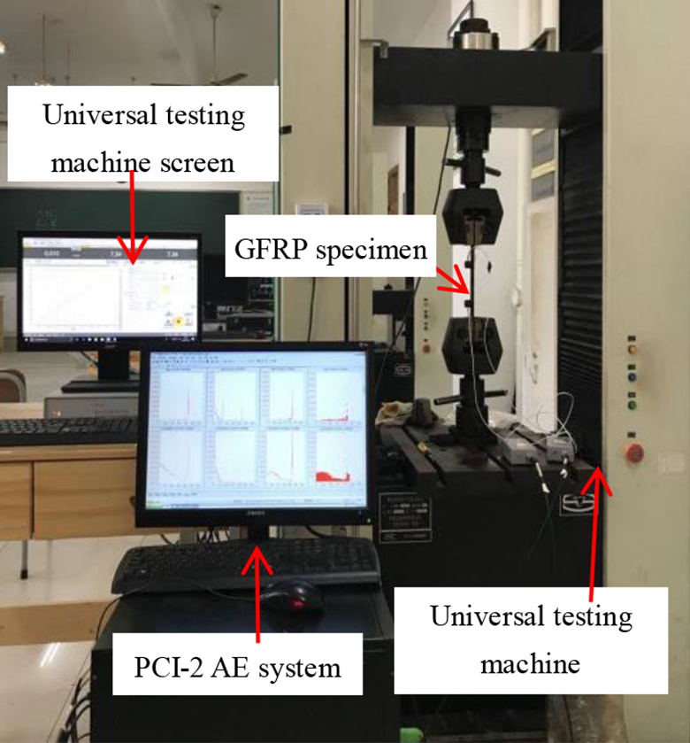
A picture of the monitoring process of the GFRP specimen tensile test. GFRP: glass fiber-reinforced plastics.

Experimental process and signals collecting

Before the tensile test, the AE sensors were fixed on the specimen, the preamplifier gain was set to 40 dB, and the universal testing machine was started without tensile loading on the specimen. To collect interfering signals in the environment, the threshold value of the AE system was set to 0 dB. A total of 200 interfering signal samples were collected. Figure 5 shows the time-domain waveform of one of the collected interfering signals.

Figure 5.

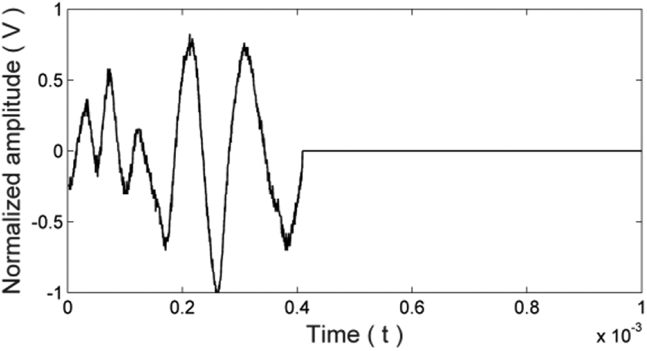
The waveform of an interfering signal.

Since the amplitudes of interfering signals were often higher than 45 dB during the collection of interfering signals, the threshold value of the AE system was set to 50 dB when the tensile test began. Then, the tensile test started to load on the specimen, extension speed was set to 1 mm/min, and the AE system started to collect the AE signals at the same time. To collect the effective AE signals, the signals that appeared near the preset gaps were mainly collected as the effective AE signal samples. A total of 200 effective AE signal samples were collected. The waveform of one of the effective AE signals is shown in Figure 6.

Figure 6.

The waveform of an effective AE signal. AE: acoustic emission.

Signal characteristics analysis

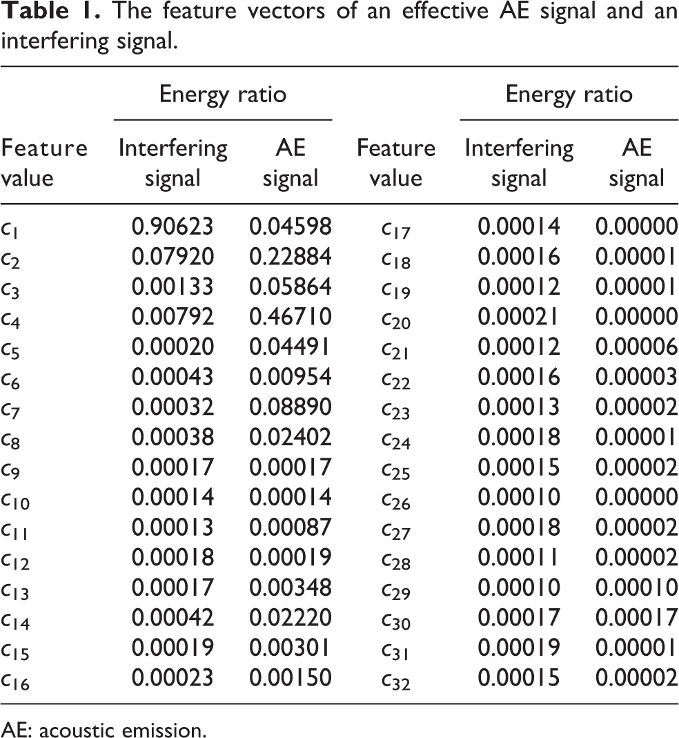
The Db4 wavelet basis was used to decompose all the collected effective AE and the interfering signals, and each signal was decomposed to the fifth layer, that is, each signal was decomposed to produce 32 reconstructed signals in different frequency ranges. The energy ratio between the energy of each reconstructed signal and the total energy of the collected signal can be calculated according to equation (4), which is composed of the feature vector C of the collected signal. Figure 7 shows the bar graphs of the feature value distribution of two randomly selected effective AE and interfering signals, respectively. The calculation results of the feature vectors are listed in Table 1, where c_i (i = 1, 2,…, 32) is the i’th feature value in the feature vector, and its value is the energy ratio of the energy of the i’th reconstructed signal to the total energy of the collected signal.

Figure 7.

The bar graph of the feature values distribution of (a) an interfering signal and (b) an effective AE signal. AE: acoustic emission.

Table 1.

The feature vectors of an effective AE signal and an interfering signal.

Feature value	Energy ratio		Feature value	Energy ratio
Feature value	Interfering signal	AE signal	Feature value	Interfering signal	AE signal
c ₁	0.90623	0.04598	c ₁₇	0.00014	0.00000
c ₂	0.07920	0.22884	c ₁₈	0.00016	0.00001
c ₃	0.00133	0.05864	c ₁₉	0.00012	0.00001
c ₄	0.00792	0.46710	c ₂₀	0.00021	0.00000
c ₅	0.00020	0.04491	c ₂₁	0.00012	0.00006
c ₆	0.00043	0.00954	c ₂₂	0.00016	0.00003
c ₇	0.00032	0.08890	c ₂₃	0.00013	0.00002
c ₈	0.00038	0.02402	c ₂₄	0.00018	0.00001
c ₉	0.00017	0.00017	c ₂₅	0.00015	0.00002
c ₁₀	0.00014	0.00014	c ₂₆	0.00010	0.00000
c ₁₁	0.00013	0.00087	c ₂₇	0.00018	0.00002
c ₁₂	0.00018	0.00019	c ₂₈	0.00011	0.00002
c ₁₃	0.00017	0.00348	c ₂₉	0.00010	0.00010
c ₁₄	0.00042	0.02220	c ₃₀	0.00017	0.00017
c ₁₅	0.00019	0.00301	c ₃₁	0.00019	0.00001
c ₁₆	0.00023	0.00150	c ₃₂	0.00015	0.00002

AE: acoustic emission.

It can be seen from Figure 7(a) that the interfering signal is mainly concentrated in the first two frequency ranges, which accounts for more than 97% of the total energy of the interfering signal. The energy in the second frequency band higher than that in the first band, accounting for about 90% of the total energy. It shows that the frequency component of the interfering signal is relatively concentrated and the main frequency range is 0–156.2 kHz.

It can be seen from Figure 7(b) that the effective AE signal energy is mainly concentrated in the first to eighth frequency range (the first to eighth feature value in the feature vector), which accounts for more than 95% of the total energy of the AE signal, while the energies in other frequency ranges are relatively low. It shows that the frequency component of the effective AE signal is mainly concentrated between 0 kHZ and 300 kHz, there are a few high-frequency components that can reach 400 kHz, and the signal covers a wide frequency range.

It can be seen from Table 1 that the wavelet packet feature vector with the five-layer decomposition divides the signal more finely, and the feature vector of two types extracted based on the wavelet packet decomposition is clearly different. The frequency of the interfering signal is significantly lower than the frequency of the AE signal. The interfering signals are unnecessary in the evaluation of AE sources and affect the evaluation results. Therefore, the interfering signals should be distinguished and removed first, and the effective AE signals should be retained for further damage evaluation.

Intelligent recognition and analysis of AE signals

In this study, the BPNN model is used to perform intelligent recognition on the AE signal feature vectors obtained by wavelet packet decomposition. The BPNN model can recognize and accurately classify the interfering and the effective AE signals and provide an evaluation basis for the retention of effective AE signals.

The signal samples included 200 interfering signals and 200 effective AE signals collected in the previous experiment, that is, a total of 400 samples. From the two types of signals, the feature vectors were obtained using the wavelet packet decomposition and 360 samples feature vectors were selected for BPNN training. The remaining 40 samples of the two types were used to verify the accuracy of the trained NN.

Figure 8 shows the training error curve of the BPNN. It can be seen from Figure 8 that the network reached the expected goal after 50 iterations of training. After training 360 signal samples of different types, the BPNN performed intelligent recognition on the remaining 40 signal samples. The statistical recognized results are shown in Figure 9. In Figure 9, output number “0” indicates that the recognized result is an interfering signal, and the output number “1” indicates that the recognized result is an effective AE signal. The marks “o” and “*” indicate the BPNN sample type and the actual collected sample type, respectively.

Figure 8.

Training error curve of the BPNN. BPNN: back-propagation neural network.

Figure 9.

Comparison diagram of signal recognized results.

It can be seen from Figure 9 that among the 40 signal samples for the intelligent recognition with BPNN, only one sample (the eighth sample) recognized result is wrong, and the other recognized results are consistent with the actual collected signal type. Therefore, the recognition accuracy of the signal type with the BPNN based on the feature vector by wavelet packet decomposition reached 97.5%, which indicates that the BPNN has strong intelligent recognition ability and high accuracy for the AE signal recognition.

Analysis and discussion of recognized results

The research focused on intelligent recognition method for the effective AE signals, which sent out from the material damage. For the recognition results, the accuracy was less than 93% when the detection parameters were directly used for BPNN.^33,34 The accuracy was 96% when the characteristic parameters extracted by wavelet decomposition were used for BPNN.³⁵ In this work, the feature vector obtained by wavelet packet decomposition was used as the input parameters of BPNN, and the recognition accuracy reaches 97.5%. Meanwhile, the number of iterations to achieve the target error was also significantly reduced. Therefore, the proposed intelligent recognition method has better accuracy and recognition efficiency by comparison.

Conclusion

In this article, a method for intelligent recognition of effective AE signals is proposed to meet the requirements of AE testing for GFRP structures. The proposed method can remove interfering signals and provide a reliable basis for further accurate evaluation of the damage. Different types of signals are decomposed to the fifth layer using the wavelet packet analysis, and the wavelet packet feature vector is calculated. It is found that the feature vectors of the two types of the collected signals are obviously different. Then, a BPNN is designed and the main network parameters, such as the number of hidden layer nodes and the transfer functions, are determined. The BPNN was trained through 360 feature vector samples obtained by collecting signals. The feature vector samples obtained from the 40 collected signals are input into the BPNN for intelligent recognition, and a recognition accuracy rate of 97.5% is achieved. The experimental results validate that the proposed method meets the requirements for accurate recognition of the effective AE signals.

Footnotes

Acknowledgments

The authors would like to thank Prof. Zheng FAN for helping us finish the paper during the visiting study in Non-Destructive Testing Lab at Nanyang Technological University, Singapore.

Declaration of conflicting interests

The author(s) declared no potential conflicts of interest with respect to the research, authorship, and/or publication of this article.

Funding

The author(s) disclosed receipt of the following financial support for the research, authorship, and/or publication of this article: This work was supported by the National Natural Science Foundation of China [Grant Nos. 11764030 and 51705232], Special Plan for the Construction of Superiority Scientific and Technological Innovation Teams in Jiangxi Province [Grant No.20171BCB24008], and Natural Science Foundation of Jiangxi Province [Grant No. 20192BAB216026].

ORCID iD

Chao Lu

References

Aslan

Tufan

Kucukomeroglu

. Tribological and mechanical performance of sisal-filled waste carbon and glass fibre hybrid composites. Compos B Eng 2018; 140: 241–249.

Hsu

Hsieh

. A study on improving the mechanical behaviors of the pultruded GFRP composite material members. Sustainability 2019; 11: 577.

Wang

Sun

, et al. Comparative study of vortex-induced vibration of FRP composite risers with large length to diameter ratio under different environmental situations. Appl Sci 2019; 9: 517.

Ciang

Lee

Bang

. Structural health monitoring for a wind turbine system: a review of damage detection methods. Meas Sci Technol 2008; 19: 122001.

Fitoussi

Bocquet

Meraghni

. Effect of the matrix behavior on the damage of ethylene-propylene glass fiber reinforced composite subjected to high strain rate tension. Compos B Eng 2013; 45: 1181–1191.

Rébillat

Hmad

Kadri

, et al. Peaks over threshold-based detector design for structural health monitoring: application to aerospace structures. Struct Health Monit 2018; 17: 91–107.

Liu

Zeng

, et al. Applications of a nanocomposite-inspired in-situ broadband ultrasonic sensor to acousto-ultrasonics-based passive and active structural health monitoring. Ultrasonics 2017; 78: 166–174.

Pawel

Maciej

Wieslaw

. Impact induced damage assessment by means of Lamb wave image processing. Mech Syst Signal Process 2018; 102: 23–36.

Luo

Long

, et al. Location method of acoustic emission by time reversal focusing and enhancing for steel plate. Chinese J Sci Instrum 2016; 8: 1792–1799.

10.

Wei

Chen

, et al. Acoustic emission source localization method for high-speed train bogie. Multimed Tools Appl 2020; 79: 14933–14949.

11.

Long

, et al. Acoustic emission monitoring and evaluation for rolled steel damage under different tensile rates. J Vib Shock 2017; 36: 219–225.

12.

Sause

MGR

Muller

Horoschenkoff

, et al. Quantification of failure mechanisms in mode-I loading of fiber reinforced plastics utilizing acoustic emission analysis. Compos Sci Technol 2012; 72: 167–174.

13.

Balan

Arumugam

Abdul Rauf

, et al. Estimation of residual flexural strength of unidirectional glass fiber reinforced plastic composite laminates under repeated impact load. J Compos Mater 2015; 49: 713–722.

14.

Chen

, et al. AE source location method based on time reversal for glass fiber reinforced plastics plate. Chinese J Sci Instrum 2020; 6: 208–217.

15.

Chen

Xie

Zhang

. Damage identification based on wavelet packet analysis method. Int J Appl Electromagn Mech 2016; 52: 407–414.

16.

Bianchi

Mayrhofer

Groschl

, et al. Wavelet packet transform for detection of single events in acoustic emission signals. Mech Syst Signal Process 2015; 64: 441–451.

17.

Xian

Zeng

. An intelligent fault diagnosis method based on wavelet packet analysis and hybrid support vector machine. Expert Syst Appl 2009; 36: 12131–12136.

18.

Caggiano

Nele

. Artificial neural networks for tool wear prediction based on sensor fusion monitoring of CFRP/CFRP stack drilling. Int J Autom Technol 2018; 3: 275–281.

19.

Wang

Dixit

Chegdani

, et al. Bidirectional gated recurrent deep learning neural networks for smart acoustic emission sensing of natural fiber-reinforced polymer composite machining process. Smart Sustain Manuf Syst 2020; 2: 179–198.

20.

Suresh Kumar

Arumugam

Sengottuvelusamy

, et al. Failure strength prediction of glass/epoxy composite laminates from acoustic emission parameters using artificial neural network. Appl Acoust 2017; 115: 32–41.

21.

Sause

MGR

Schmitt

Kalafat

. Failure load prediction for fiber-reinforced composites based on acoustic emission. Compos Sci Technol 2018; 164: 24–33.

22.

Brunner

AJ.

Fiber-reinforced polymer composites test specimen design for selected damage mechanisms. Proc Institut Mech Eng Part L: J Mater Des Appl 2019; 3: 328–337.

23.

Nair

Cai

Kong

. Acoustic emission pattern recognition in CFRP retrofitted RC beams for failure mode identification. Compos B Eng 2019; 161: 691–701.

24.

Nair

Cai

Kong

. Studying failure modes of GFRP laminate coupons using AE pattern-recognition method. J Aerosp Eng 2019; 4. DOI: 10.1061/(ASCE)AS.1943-5525.0001015.

25.

Rumelhartand

McClelland

. Parallel distributed processing: explorations in the microstructure of cognition. Cambridge: MIT Press, 1987, pp. 14–23.

26.

Lan

Sun

. Application of BP neural network fault diagnosis in solar photovoltaic system. In: 2009 international conference on mechatronics and automation, Changchun, China, 9–12 August 2009, pp. 2581–2585. DOI: 10.1109/ICMA.2009.5246742.

27.

Eric

. BP neural network-based effective fault localization. Int J Softw Eng Knowl Eng 2009; 19: 573–597.

28.

Zhang

. Feature extraction using wavelet packet decomposition based on MPEG-I. In: 2008 9th international conference on signal processing, Beijing, China, 26–29 October 2008, pp. 2233–2237. DOI: 10.1109/ICOSP.2008.4697593.

29.

Keskes

Braham

Lachiri

. Broken rotor bar diagnosis in induction machines through stationary wavelet packet transform and multiclass wavelet SVM. Electr Power Syst Res 2013; 97: 151–157.

30.

Wang

Liang

. Wavelet packet energy characterization of low velocity impacts and load localization by optical fiber Bragg grating sensor technique. Appl Opt 2013; 52: 2346–2352.

31.

Kang

Song

. Neural network applications in determining the fatigue crack opening load. Int J Fatigue 1998; 20: 57–69.

32.

Cheng

Shi

, et al. Brief introduction of back propagation (BP) neural network algorithm and its improvement. In: Jin

Lin

(eds) Advances in computer science and information engineering. Advances in intelligent and soft computing. Berlin, Heidelberg: Springer, 2012, Vol. 169, pp. 553–558. DOI: 10.1007/978-3-642-30223-7_87.

33.

. The application of improved back propagation neural network model. Comp Model New Technol 2014; 12: 34–39.

34.

Peng

Xiong

, et al. Facile preparation of a ZnO/SnO₂-based gas sensor array by inkjet printing for gas analysis with BPNN. J Electron Mater 2019; 4: 2373–2381.

35.

Wang

Zhang

, et al. Multi-scale analysis and pattern recognition of ultrasonic signals of PD in a liquid/solid composite of an oil-filled terminal. Energies 2020: 13: 366.

Intelligent recognition of acoustic emission signals from damage of glass fiber-reinforced plastics

Abstract

Keywords

Introduction

Recognition principle

Wavelet packet analysis principle

Back-propagation neural network

Experimental testing and analysis

Specimen preparation

Experimental system

Experimental process and signals collecting

Signal characteristics analysis

Intelligent recognition and analysis of AE signals

Analysis and discussion of recognized results

Conclusion

Footnotes

Acknowledgments

Declaration of conflicting interests

Funding

ORCID iD

References