Tool reliability of sintered diamond drill bit for processing silicon carbide ceramics based on Bayesian theory

Abstract

Silicon carbide (SiC) ceramics, as a superhard nonmetallic material, would induce severe tool wear during drilling. To ensure the quality of processing, the drill bits must be replaced in advance before failure, which leads to serious waste without effective usage. Aiming at the tool reliability problem determined by the tool wear during drilling of the high hardness nonmetallic materials, this article proposed a reliability analysis method of sintered diamond drill bit for machining SiC ceramics based on the distribution of tool degradation increment and the modeling of gamma process, and a tool reliability model of degradation increment was established based on the Bayesian theory. The drilling experiment of sintered SiC ceramics was carried out by sintering diamond drill bit to obtain the degradation increment data. The accuracy of the model was tested by the reliability model deviation rate, which indicated that the reliability model with considering individual differences was more accurate. This research can provide a theoretical model and analytical method for improving the reliability of the nonmetallic brittle material processing tools.

Introduction

Silicon carbide (SiC) ceramics are widely used in petrochemical, automotive, mechanical, and aerospace industries due to their excellent thermal shock resistance, high temperature resistance, oxidation resistance, and chemical corrosion resistance. However, as a nonmetallic hard material, the main tool failure form of processing SiC ceramics is severe fatigue wear. Knowing the reliability of the tool in time is an effective way to prevent the use of severely worn tools resulting in a sharp decline in the quality of the machining or premature tool replacement resulting in tool underuse.

The identification and description of tool condition are extremely important to estimate tool residual life and tool reliability. Guo et al. ¹ proposed a discrete dynamic reliability evaluation equation based on the progressive wear process to identify the tool’s wear state in the process of machining. Aramesh et al. ² established a Weibull risk model using the actual tool wear value during turning titanium metal matrix composite (Ti-MMC). By comprehensively considering the influence of the tool wear, cutting speed and feed speed, the accuracy and reliability of the model were verified through the experiments. Wang et al. ³ proposed a tool residual life prediction method of the Gaussian distribution based on a reliable identification of the milling tool wear state and conducted the diagnosis of the tool wear state using the cutting force signals. Hsu and Shu ⁴ established a tool reliability evaluation model under different wear conditions based on nonhomogeneous continuous time Markov process.

In the process of the tool wear state diagnosis, there are many modeling methods for estimating the tool reliability and remaining life, such as different distribution functions or Bayesian theory, Markov model, fuzzy reliability estimation, ⁵ neural network, ⁶ and logistic regression model. ⁷ Li and Liu ⁸ used the improved hidden Markov model to establish a risk model that could describe the probability of time-varying and the conditional adaptive state transition to predict the tool remaining life under different cutting conditions, and the model’s feasibility was tested by T4 steel processing experiments on CNC machine. Yu et al. ⁹ proposed a tool life prediction method based on weighted hidden Markov model, which was verified the higher accuracy than the traditional Markov model by collecting data from high-speed CNC milling experiment. Tao et al. ¹⁰ proposed a prediction model for the tool residual life based on the short-time memory network and hidden Markov combination. Benkedjouh et al. ¹¹ put forward a tool residual life prediction model based on nonlinear feature reduction and support vector regression. Cui et al. ¹² provided a performance indicator of the tool by combining the effects of the original damage of the tool material microstructure, the macromechanical properties of the tool material, and the external loads on the cutting tool. The reliability of ceramic cutting tools is analyzed under two cutting conditions of superhard materials (intermittent and continuous). The results showed that the tool performance indicator and the tool life were subject to Weibull distribution. Wang et al. ¹³ established a dynamic reliability sensitivity model of cemented carbide tools based on the influence of physical properties of cemented carbide materials. It can determine the influence of tool parameters, such as tool material and physical properties, on tool reliability. Salonitis and Kolios ¹⁴ built a tool reliability model based on the advanced approximation method with integrated stochastic response surface, surrogate modeling, and Monte Carlo simulations. Aramesh et al. ¹⁵ set up a reliability model for machining titanium metal matrix composites (TI-MMCs) based on the reliability function and mean time to failure. The reliability models established by the above methods were all applied to metal working tools. However, there is a big difference in the drilling mechanism between the superhard nonmetallic materials and metallic materials. Research on the tool reliability of drill bit for machining superhard nonmetals has hardly been carried out.

Therefore, a reliability analysis method established by the tool distribution of degradation increment and the modeling of gamma process were proposed based on Bayesian theory. The single-factor hole drilling experiment of sintered SiC ceramics was carried out by sintered diamond drill bit to obtain the degradation increment data. The reliability of the drill bit was investigated by collecting tool wear increment and analyzing its relationship with cutting force. This research is expected to provide the theoretical model and analytical method to improve the tool reliability of drilling hard nonmetallic materials.

Reliability modeling method

Bayesian method and Markov chain Monte Carlo

By systematic considering sample information, prior information, and general information, Bayesian method has been widely used in various fields. In Bayesian theory, the unknown parameter θ is regarded as a random variable and described by a probability distribution, which is called the prior distribution. A new distribution about the unknown parameter θ is obtained by taking the sample information and the information on the population distribution and the prior distribution. The new distribution is called the posterior distribution. The posterior distribution of equation (1) is established according to reference ¹⁶

$\pi \left(\theta |x\right)=\frac{f\left(x|\theta \right)\pi \left(\theta \right)}{m\left(x\right)}$

1

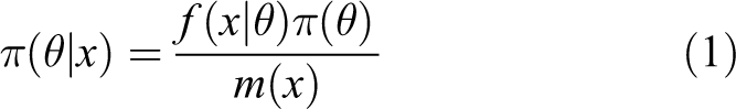
where π(θ|x) represents the posterior distribution of model parameters, f(|θ) is the density of simultaneous distribution of the samples, π(θ) is prior distribution, and m(x) is the marginal density of x. Here

$m\left(x\right)={\displaystyle \underset{\Theta }{\int }f\left(x|\theta \right)}\pi \left(\theta \right)\hspace{0.17em}\text{d}\theta \hspace{0.17em}\to \left(\theta \mathit{Î}\Theta \right)\left(\Theta \hspace{0.17em}\text{is parameter space}\right)$

2

Since m(x) is independent of θ, the likelihood function l(x|θ) can be substituted in some cases; then, the posterior distribution can be approximately expressed as

$\pi \left(\theta |x\right)\propto l\left(x|\theta \right)\pi \left(\theta \right)$

3

In practical terms, the posterior distribution is very complex, moreover, its analytical expression is not easy to obtain. To solve this problem, some random simulation methods are often used to estimate relevant parameters. Markov chain Monte Carlo (MCMC) is one of the methods to calculate high dimensional integrals based on the basic idea of simulating the sample path of Markov chain. After sufficient iteration, the Markov chain converges to a stationary target distribution and the sample of the posterior distribution is obtained. Those samples will be used for subsequent calculations and inferences. ¹⁷

Reliability modeling based on gamma process

Reliability modeling of product degradation process based on random process usually takes the product degradation process as a random event. For sintered diamond drill bits, the tool failure is mainly in the form of wear and damage. However, under the premise of reasonable selection of processing parameters, the probability of wear is far greater than that of damage. With the increasing of tool wear amount, tool performance deteriorates and tool reliability decreases. Therefore, the tool wear amount is chosen as the tool performance index. As a random process, tool wear increment is non-negative and independent, which is ideal for the main indicator of reliability modeling. Since the gamma process is an independent, incremental non-negative random process, it has been widely used in reliability modeling, which is in line with the characteristics of the wear degradation increment of sintered diamond bits. Therefore, the gamma process is selected for the reliability modeling of tool degradation failure. The definition of the gamma process Ga (α(t), λ) ¹⁸ is as following.

If the density function of the random variable X is

$f\left(x;\alpha ,\lambda \right)=\left\{\begin{array}{ll}\frac{{\lambda }^{\alpha }}{\Gamma \left(\alpha \right)}{x}^{\alpha -1}{e}^{-\lambda x}\text{,}& x>0\\ \mathrm{0,}& x\le 0\end{array}\right.$

4

where X follows the gamma distribution and is denoted as X∼Ga(α, λ), α > 0, λ > 0. α is the shape parameter and λ ⁻¹ is the scale parameter, here

$\Gamma \left(\alpha \right)={\displaystyle {\int }_0^{+\infty }{x}^{\alpha -1}}{e}^{-\lambda x}\text{d}x$

5

If the random process {X(t), t > 0} meets the following three conditions:

1. X(0) = 0;

2. Obey the gamma distribution, as illustrated by equation (6)

   $X(\tau )-X(t)\text{∼}Ga\left(\alpha (\tau )-\alpha (t),\beta \right),\tau >t\ge 0,\hspace{0.17em}\left(\tau ,t\hspace{0.17em}\text{is time}\right)$

   6

3. X(t) is the independent increment.

Then, the random process{X(t), t > 0} is called the gamma process, where the shape parameter of the gamma distribution α(t) can be selected according to different random processes. When the function α(t) is linear, the gamma process is a stationary random process. When α(t) is a nonlinear function, the gamma process is an unstable process.

In summary, the probability density of the gamma process {X(t), t > 0} is

$f\left(x;\alpha \left(t\right),\lambda \right)=\left\{\begin{array}{ll}\frac{{\lambda }^{\alpha (t)}}{\Gamma \left(\alpha \left(t\right)\right)}{x}^{\alpha (t)-1}{e}^{-\lambda x}\text{,}& x>0\\ 0,& x\le 0\end{array}\right.$

7

The distribution fitting of the tool degradation data is performed to verify that the gamma process is an appropriate random process. The tool wear data are imported into the SPSS software (version 22) and analyzed using the P–P plot in SPSS, and the goodness of fit is determined by the residual value of fitting. The Weibull distribution, exponential distribution, normal distribution, lognormal distribution, and gamma distribution are fitted to the tool wear data, respectively. Then, the goodness of fit test is carried out and the χ ² test theory is adopted to check whether the observed data are consistent with the theoretical values of a probability distribution.

The modeling method established by the gamma process based on Bayesian theory is shown in Figure 1.

Figure 1.

The flowchart of reliability modeling based on gamma process.

Reliability modeling of gamma processes without considering individual differences

The modeling process can be simplified by ignoring individual differences between the sintered diamond bits.

1. Gamma process modeling without considering individual differences

The gamma process describes various monotonous product degradation processes using different shape parameters α(t). In practice, the product degradation should have a degradation indicator. When the degradation amount reaches a certain level, it is judged as the product failure. Therefore, the degradation indicator is the failure threshold D and the product life is denoted as T.

Let {X(t), t ≥ 0} be the gamma process, then, the product life T

$T=\text{inf}\left\{t|X(t)\ge D\right\}$

8

The reliability of the product R(t) at t moment is

$R\left(t\right)=\text{Pr}\left\{X(t)<D\right\}$

9

Since the gamma process is monotonically increasing, the product reliability can be obtained by combining equation (3) with equation (7)

$R(t)=\frac{{\displaystyle \underset{0}{\overset{D\lambda }{\int }}{u}^{\alpha (t)-1}{e}^{-u}}\text{d}u}{\Gamma \left(\alpha \left(t\right)\right)}$

10

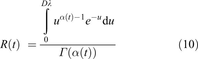
where λ is the reciprocal of the λ ⁻¹. The distribution function and probability density function of product life T are as follows

$F(t)=1-R\left(t\right)=1-\frac{{\displaystyle \underset{0}{\overset{D\lambda }{\int }}{u}^{\alpha (t)-1}{e}^{-u}}\text{d}x}{\Gamma \left(\alpha \left(t\right)\right)}$

11

$f\left(t\right)=\frac{{\alpha }^{\prime }\left(t\right)}{\Gamma \left(\alpha \left(t\right)\right)}{\displaystyle \underset{D\lambda }{\overset{\infty }{\int }}\left\{\text{log}\left(u\right)-\phi \left(\alpha \left(t\right)\right)\right\}{u}^{\alpha (t)-1}{e}^{-u}\text{d}u}$

12

where α′(t) is derivative of α(t) to t, φ(α(t)) is derivative of log(Γ(α(t))) to α(t).

• 2. Bayesian parameter estimation without considering individual differences

There are N tool increment samples with the sample number of i = 1, 2, 3,…, N. The sample x_i (the ith sample increment) obeys Ga(α(t), λ), α(t) = ηt, and η is the estimate parameters.

The likelihood function of sample X is

$L\left(X;\theta \right)={\displaystyle \prod _{i=1}^n\frac{{\lambda }^{\alpha (t)}}{\Gamma \left(\alpha \left(t\right)\right)}}{x}_i{}^{\alpha (t)-1}{e}^{-\lambda x_i}$

13

The reliability equation based on Bayesian posterior distribution is

$R_{RD}\left(t|X_{RD}\right)={\displaystyle \underset{\theta }{\int }{R}_{RD}\left(t|\theta \right)P\left(\theta |X_{RD}\right)}\hspace{0.17em}\text{d}\theta$

14

where X_RD is a degradation data set, and, in this article, it is the tool wear increment data set. R_RD (t|θ) is obtained from equation (10), and P(θ|X_RD ) is the joint posterior distribution of the parameters. According to equation (3), P(θ|X_RD ) can be given as

$P\left(\theta |X_{RD}\right)\propto L\left(X_{RD};\theta \right)\pi \left(\theta \right)$

15

where π(θ) is the joint prior distribution of relevant parameters, π(θ) = π(η, λ).

Combine with equations (10), (14), and (15), R_RD (t|X_RD ) can be derived as

$R_{RD}\left(t|X_{RD}\right)={\displaystyle \underset{\theta }{\int }{R}_{RD}}\left(t|\alpha \left(t\right),\lambda \right)\pi \left(\alpha \left(t\right),\lambda \right){\displaystyle \prod _{i=1}^n\frac{{\lambda }^{\alpha (t)}}{\Gamma \left(\alpha \left(t\right)\right)}}{x}_i{}^{\alpha (t)-1}{e}^{-\lambda x_i}\text{d}\theta$

16

Reliability modeling of gamma processes with considering individual differences

• 1. Gamma process modeling with considering individual differences

The degradation process of different tools under the same processing condition is different because of the manufacturing error between individual tools and workpieces, the difference in the processing environment, and the clamping standard of tools. Therefore, under the same processing condition, the degradation process of different tools can be better described by considering the individual differences.

Set the gamma process as {x(t), t ≥ 0}, the shape parameter as α(t) = ηt, and the scale parameter as υ ⁻¹. ΔX(t) is the increment of X(t) in Δt moment. According to the gamma process definition, the relationship is as follows:

$\Delta X\left(t\right)\sim Ga\left(\eta \Delta t,{\nu }^{-1}\right)$

17

The individual differences of products are assumed to affect only the scale parameters υ ⁻¹. In other words, different scale parameters are used to describe the degradation process between different individuals under the same condition. The scale parameter υ ⁻¹ obeys another gamma process in which the shape parameter is δ and the scale parameter is γ ⁻¹. That is

$\nu \sim Ga\left(\delta ,{\gamma }^{-1}\right)$

18

X(t) is monotonically increasing; δx(t)/(γηt) obeys the F distribution and is written as F_2ηn,2δ (x). Then, the cumulative density function of product degradation process in time T is

$\begin{array}{l}{F}_0\left(t\right)=P\left(T\le t\right)\\ =\frac{B\left(Y;\eta t,\delta \right)}{B\left(\eta t,\delta \right)}\end{array}$

19

where $B\left(x;a,b\right)={{\displaystyle {\int }_x^1{z}^{a-1}\left(1-z\right)}}^{b-1}\text{d}z$ , Y = X(T)/(X(T) + γ), and B(a, b) is complete β function.

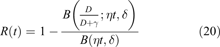
Combined with equation (17), the reliability of the product at moment t is

$R\left(t\right)=1-\frac{B\left(\frac{D}{D+\gamma };\eta t,\delta \right)}{B\left(\eta t,\delta \right)}$

20

• 2. Bayesian parameter estimation with considering individual differences

There are N tool increment samples with the sample number of i = 1, 2, 3,…, N. The degradation increment is measured in M times for each sample and the serial number is j(j = 1, 2…, M). t_ij is the time of the jth measurement of the ith sample. X(t_ij ) is the degradation increment at this point, and X(t_i0 ) is the initial degradation increment of the i’th sample. Thus, the degradation increment of the i’th sample is

$x_{ij}=X\left(t_{ij}\right)-X\left(t_{i,j-1}\right)$

21

Combining equation (18), X is the sample information of the observed sample. Then, the likelihood function based on X is

$L\left(X,\nu |\theta \right)={\displaystyle \prod _{i=1}^N\frac{v_i{}^{\delta -1}{\gamma }^{\delta }}{\Gamma \left(\delta \right)}}{e}^{-\gamma v_i}{\displaystyle \prod _{j=2}^M\frac{{\left(\Delta x_{ij}\right)}^{\eta \Delta t_{ij}-1}{v}_i{}^{\eta \Delta t_{ij}}}{\Gamma \left(\eta \Delta t_{ij}\right)}}{e}^{-v_i\Delta x_{ij}}$

22

where $\Delta t_{ij}=t_{ij}-t_{ij-1}$ , ${\nu }_i^{-1}$ is the scale parameter of each sample.

According to equation (3), the posterior distribution is

$\begin{array}{l}p\left(\eta ,\delta ,\gamma ,v\right)\propto L\left(X,v|\theta \right)\pi \left(\theta \right)\\ =\pi \left(\eta ,\delta ,\gamma \right){\displaystyle \prod _{i=1}^N\frac{v_i{}^{\delta -1}{\gamma }^{\delta }}{\Gamma (\delta )}}{e}^{-\gamma v_i}{\displaystyle \prod _{j=2}^M\frac{{\left(\Delta x_{ij}\right)}^{\eta \Delta t_{ij}-1}{v}_i{}^{\eta \Delta t_{ij}}}{\Gamma \left(\eta \Delta t_{ij}\right)}}{e}^{-v_i\Delta x_{ij}}\end{array}$

23

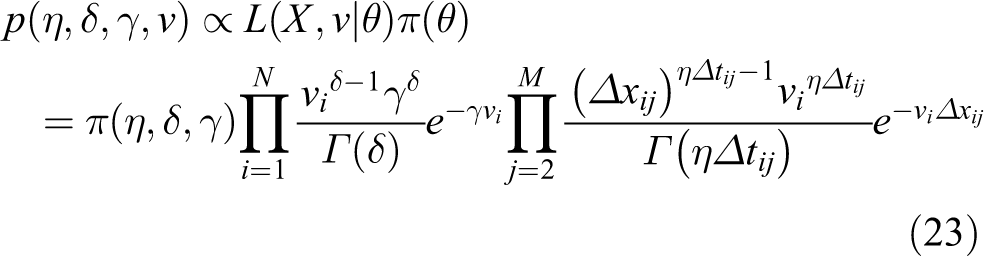
where π(θ) = π(η, δ, γ) is the joint prior distribution of all parameters, π(θ|x) = P(η, δ, γ, υ) is the joint posterior distribution of each parameter.

Combining equations (20) and (23), the reliability of the product is

$R\left(t|X\right)={\displaystyle \underset{\eta ,\delta ,\gamma >0}{\int }p\left(\eta ,\delta ,\gamma |X\right)}\frac{B\left(D/(D+\gamma );\eta t,\delta \right)}{B\left(\eta t,\delta \right)}\hspace{0.17em}\text{d}\eta \text{d}\delta \text{d}\gamma$

24

Case study

Experimental setup

Experimental schedule

Without considering the difference of diamond tool manufacture and materials, tool wear of SiC ceramics drilled by diamond drill bit mainly depends on cutting parameters (spindle speed, depth of cut, and feed speed). Since the degradation data collected in this experiment was the tool wear amount after tool grinding for a fixed length of time and the cutting depth under the same feed speed was the same, the impact of the depth of cut on tool wear was not considered in this article. The single factor experiment method was used, and the experimental processing method was straight drilling with the Castrol llocut154 pure oil cooling of 120 cm³/min flow rate.

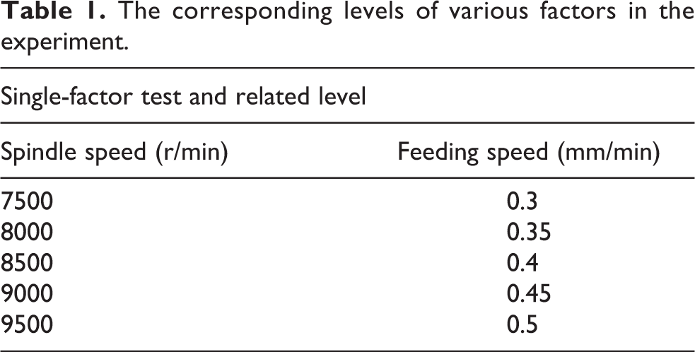
After sufficient pretests, the range of processing parameters is presented in Table 1. Table 2 presents the experimental scheme of the influence of cutting parameters on tool wear.

Table 1.

The corresponding levels of various factors in the experiment.

Single-factor test and related level
Spindle speed (r/min)	Feeding speed (mm/min)
7500	0.3
8000	0.35
8500	0.4
9000	0.45
9500	0.5

Table 2.

The experimental scheme of the influence of cutting parameters on tool wear.

Serial number	Spindle speed (r/min)	Feeding speed (mm/min)
1–5	7500–9000	0.3
6–10	7500–9000	0.4
11–15	7500–900	0.5
16–20	7500	0.3∼0.5
21–25	8500	0.3∼0.5
26–30	9500	0.3∼0.5

The experimental scheme of tool reliability is provided in Table 3. Each set of parameters was tested by three different drill bits produced in the same batch (named as drill bits 1, 2, and 3). Each drill bit was continuously used for eight times for 15 min at a time, and the quality change of mass was measured before and after every 15 min of drilling.

Table 3.

The continuous wear test scheme of cutting tools.

Serial number	Spindle speed (r/min)	Feeding speed (mm/min)
1	8000	0.3
2	8500	0.3
3	8000	0.4
4	8500	0.4
5	8000	0.5
6	8500	0.5

Experimental system equipment and materials

• 1. Machine tool selection

The experimental platform is shown in Figure 2. The FANUC ROBODRILL_α-T14iFLb machining center was used in this experiment. It has a maximum speed of 24,000 r/min and a spindle power of 11 kW/3.7 kW.

Figure 2.

The experimental platform.

• 2. Tools

The sintered diamond drill bit with a diamond size of 80/100 produced by Zhengzhou Zhongtuo Abrasive Tools Co. Ltd (China) was used in this experiment. Its matrix material is SKD12 high-speed steel after tempering treatment, and its hardness is 65HRC, as seen in Figure 3(c).

Figure 3.

SiC ceramics samples and schematic diagram of diamond bit: (a) before processing, (b) after processing, and (c) sintered diamond drill bit. SiC: silicon carbide.

• 3. Workpiece material

The workpiece is 50 × 50 × 60 mm³ nonpressure-sintered SiC ceramics produced by Hangzhou Xinfeida Electronics Co. Ltd (China). The mechanical properties of SiC ceramics are presented in Table 4.

Table 4.

The mechanical properties of SiC ceramics.

Material	Volume density (cm3)	Purity (%)	Bending strength (MPa)	Rockwell hardness (HRA)	Thermal conductivity (W(m·k))	Elastic modulus (GPa)	Fracture toughness (MPa·m1/2)
SiC	>3.12	98.5%	>400	>93	148	415	>4.5

SiC: silicon carbide.

• 4. Tool wear measurement

The quality change of each drill bit was measured by FA2204 ultra-precision electronic balance with the resolution of 0.1 mg before and after drilling for 15 min under each set of parameters. To ensure the accuracy of weighing, the drill bit was cleaned with 75% alcohol and dried before measured.

• 5. Cutting force measurement

The cutting force was collected by Kistler 9257B piezoelectric sensor and Kistler 5070A charge amplifier with the sampling frequency of 5000 Hz.

Experimental result and discussion

In the SiC drilling processing, the cutting force describes the tool wear state in one way, and the amount of tool wear directly describes the degradation process of tool performance in another way. Therefore, the tool wear is taken as the direct index to evaluate the tool reliability analysis, and the cutting force index is used to monitor the machining process from the side.

Amount of tool wear

Traditional tool wear measurement methods mainly use tool wear width (VB) and wear zone area (AVB) to evaluate the degree of tool wear. While the structure of sintered diamond drill bit adopted in this article is quite different from that of ordinary drill bits, which is mainly composed of side wear of working layer and bottom wear. Therefore, it is not suitable to evaluate tool wear by VB or AVB. Because SiC ceramics are less likely to stick to the drill bit during the processing, it is feasible to evaluate the tool wear by the quality change before and after drilling. The tool wear ratio is defined as E, where

$E=\frac{\Delta M}{L}$

25

Here, ΔM is the quality change before and after drilling, L = nh is the total depth of the hole, n is the number of holes, and h is the thickness of workpiece.

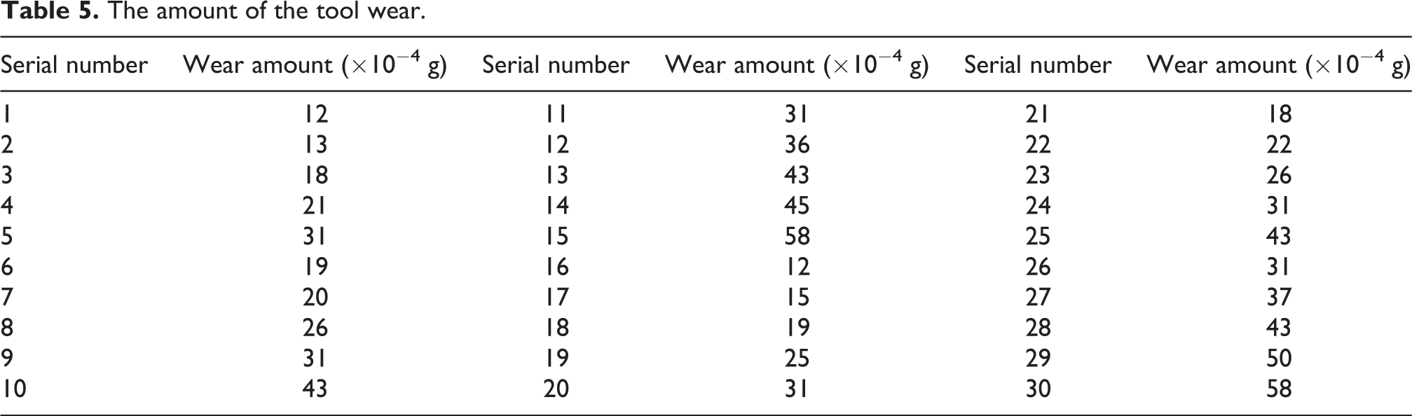
The measured values of tool wear under each cutting parameter are provided in Table 5.

Table 5.

The amount of the tool wear.

Serial number	Wear amount (×10−4 g)	Serial number	Wear amount (×10−4 g)	Serial number	Wear amount (×10−4 g)
1	12	11	31	21	18
2	13	12	36	22	22
3	18	13	43	23	26
4	21	14	45	24	31
5	31	15	58	25	43
6	19	16	12	26	31
7	20	17	15	27	37
8	26	18	19	28	43
9	31	19	25	29	50
10	43	20	31	30	58

According to the equation (25), the tool wear ratio is obtained in Figure 4, which the drilling depth was $S=V_{\text{f}}\times t$ (V _f is the feeding speed and t is the drilling time).

Figure 4.

The tool wear ratio.

Analysis of influencing factors of tool wear

• 1. Effects of machining parameters on tool wear

The variation trend of tool wear ratio with the change of spindle speed was shown in Figure 5. When the spindle speed was between 7500 r/min and 9500 r/min, the tool wear ratio increased and the tool wear worsened. This was because the number of grinding per unit time of diamond abrasive particles increased with the increase of the main speed, which fastened the tool wear. At the same time, with the increase of spindle speed, the normal force F_t and tangential force F_n of diamond abrasive grains increased, the abrasive grains broke or fell off, and the matrix grinded workpiece together with diamond abrasive, which aggravated the tool wear. The accumulation of heat in the drilling processing led to oxidation wear and carbonization reaction, which induced the sharp increase of tool wear.

Figure 5.

Effect of spindle speed on tool wear under different feed speeds.

Figure 6 showed the effect of feed speed on tool wear ratio. The tool wear ratio increased with the increase of feed speed. With the increase of feed speed, the axial pressure and friction between the diamond abrasives and the workpiece increased accordingly.

Figure 6.

Effect of feed speed on tool wear under different spindle speeds.

• 2. Effect of cutting force on tool wear

Taking the data in Table 6 as an example, the cutting force and the tool wear increment are analyzed in Figure 7.

Figure 7.

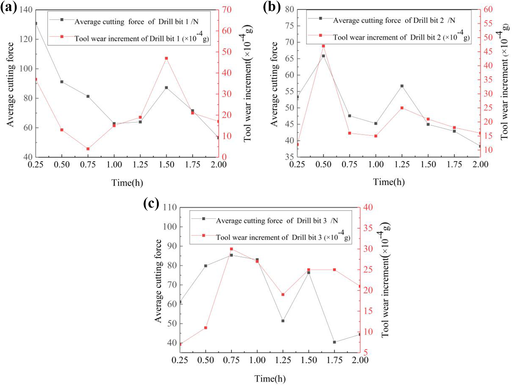
The average cutting force and tool wear increment of different drill bit: (a) drill bit 1, (b) drill bit 2, and (c) drill bit 3.

Table 6.

The increment of tool wear (n = 8500 r/min, V _f = 0.5 mm/min).

Measuring time	Tool wear increment (×10−4 g)
t (h)	Drill bit 1	Drill bit 2	Drill bit 3
0.25	37	12	7
0.5	13	47	11
0.75	4	16	30
1	15	15	27
1.25	19	25	19
1.5	47	21	25
1.75	21	18	25
2	17	16	21

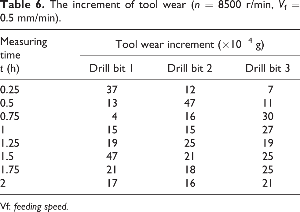
Vf: feeding speed.

Within a certain time range, the trend of the average cutting force changing with time was generally consistent with the trend of tool wear with time, and the tool wear was generally correlated with the average cutting force. It indicated that the cutting force had direct effect on the tool wear. When the cutting force increased, the extrusion force between the cutting tool and the workpiece increased, which may lead to the crushing or falling off of the diamond abrasives, and the extrusion height of diamond abrasives decreased dramatically.

Fitting and testing of tool wear increment distribution based on gamma process

• 1. Fitting of tool wear increment

The increment of tool wear is provided in Table 6. By comparing the fitting deviations of the normal distribution, exponential distribution, Weibull distribution, lognormal distribution, and gamma distribution of drill bit 1. The gamma distribution was found to be a good description of tool wear increment. After the fitting was completed, the χ2 test was used to test the statistical significance of the fitting. Its result showed that p = 0.998 of the asymptotic significance (two-side test) was significantly greater than the given significance level of α = 0.05. Therefore, it was appropriate to use a gamma distribution to descript the tool wear increment.

• 2. Tool reliability analysis without considering individual differences

Taking the tool wear increment in Table 6 as an example, combined with the results of “Fitting of tool wear increment” section, the reliability analysis of the experimental tool was conducted according to the reliability modeling method of “Reliability modeling of gamma processes without considering individual differences” section. Considering the actual processing condition and the experience of manufacturers, the tool failure threshold was set to 150 × 10⁻⁴ g in this article.

The x_ij∼Ga(α(t), λ) was known from “Reliability modeling of gamma processes without considering individual differences” section, where α(t) = ηt(η > 0) is a linear model. According to the literature, ¹⁶ the prior distribution of the two parameters was α∼U(0,50) and λ∼U(0,100).

The parameters of tool degradation model were updated using Bayesian theory. The MCMC simulation method was used to generate samples of the posterior parameters and update the parameters of the tool degradation model with the help of OpenBUGS software (version 3.2.3 rev 1012). A total of 50,000 model parameters of the posterior distribution of samples were achieved, in which previous 10,000 samples were used to ensure the convergence of the MCMC. The estimated values of η = 0.0826 and λ = 7.347 were obtained from the posterior samples and substituted into equation (10) to obtain the trend of tool reliability over time, as shown in Figure 8.

Figure 8.

The tool reliability without considering individual differences over time.

Based on the curve of tool reliability in Figure 8, the tool reliability can be calculated at any moment, while the curve of tool reliability based on the distribution of degradation increment had some defects due to the uncertain distribution of tool failure life. This also indicated that it was better to use a random process to describe the tool reliability in the case of uncertain tool failure life distribution.

• 3. Tool reliability analysis with considering individual differences

According to the literature, ¹⁶ the prior distribution of the two parameters is δ∼Ga(10,64), γ∼Ga(64,100), and η∼U(0,50). The same OpenBUGS software was used to generate tool model parameter samples. The first 10,000 samples of a total of 50,000 samples were used to ensure the convergence of the MCMC. The estimated values of model parameters obtained were provided in Table 7.

Table 7.

The estimated results of parameters.

Parameters	η	δ	γ	υ 1	υ 2	υ 3
Value	0.05726	58.312	9.1945	6.571	7.012	6.249

The parameters estimated in Table 7 were substituted into equation (20) to obtain the trend of tool reliability over time, as shown in Figure 9.

Figure 9.

The tool reliability with considering individual differences over time.

Comparing the tool reliability curve in Figures 8 and 9, it could be found that there were great differences in the tool reliability at the same time. Therefore, it was necessary to verify the validity of the model. If R_T is the reliability based on the actual tool wear amount until failure, which is taken for the actual value, R _with and R _without are the reliability with and without considering individual differences, respectively, the reliability model deviation rate P of the two models is

$P_{\text{with}}=\frac{\left|R_{\mathit{with}}-R_T\right|}{R_T}\times 100\%$

26

$P_{\text{without}}=\frac{\left|R_{\mathit{without}}-R_T\right|}{R_T}\times 100\%$

27

where P _with and P _without are the model deviation rates with and without considering individual differences.

The reliability and deviation rate of drill bit 2 at different time under different models are presented in Table 8. As could be seen in Table 8, the reliability model deviation rates with considering individual differences were all smaller than that without considering individual differences except at 0.5 h, which indicated that the model was more accurate. As a result, the reliability model with considering individual differences should be adopted when tool manufacturing errors, machining environment differences, tool clamping standards, and manufacturing errors between the workpiece and the clamping differences are large. In the case that the influence of the above situation is not significant, the reliability model without considering individual differences should be adopted to reduce the calculating amount, which could improve the calculation speed and facilitate the realization of online monitoring.

Table 8.

The reliability of drill bit 2 at each measuring time under three models.

Time (h)	R T	R without	P without (%)	R with	P with (%)
0.25	0.977	0.917	6.1	0.982	0.5
0.5	0.832	0.848	1.9	0.863	3.7
0.75	0.699	0.798	14.2	0.622	11.0
1	0.539	0.657	21.9	0.491	8.9
1.25	0.27	0.485	79.6	0.251	7.0
1.5	0.114	0.203	78.1	0.115	0.9
1.75	0.044	0.084	90.9	0.058	31.8
2	0.036	0.056	55.6	0.028	22.2

Conclusion

Based on the Bayesian theory, a reliability analysis method based on the distribution of degradation increment and the modeling of gamma process was proposed. The characteristics of drill bit wear increment were extracted by single-factor small hole drilling experiment on nonpressure sintered SiC ceramics with sintered diamond drill bit.

1. The random process of degradation of sintered diamond drill bit was described as a gamma process with tool wear increment as an indicator. On the basis of posterior distribution of Bayesian theory, the model parameters were obtained by using the MCMC. The reliability models based on the distribution of degradation increment and the gamma process without and with considering individual differences were established.

2. The tool wear ratio increased with the increase of spindle speed. With the increase of feed speed, the axial pressure and friction between the diamond abrasives and the workpiece increased accordingly, which would aggravate the tool wear. There was a correlation between the tool wear and the average cutting force, increased cutting force would lead to increased wear.

3. Based on the model of tool reliability without considering individual differences, the prediction of tool reliability can be calculated at any machining moment. When the distribution of tool failure life is uncertain, the reliability of tool is better described by random process.

4. When there was a large difference between drill bits, the reliability model with considering individual differences was more accurate than that without individual differences by comparing reliability model deviation rate to the experiment tested reliability. The reliability model considering individual differences should be adopted when manufacturing errors, machining environment differences, tool clamping standards, manufacturing errors between workpiece and clamping differences were large. In the case that the influence of the above situation is not significant, the reliability model without considering individual differences should be adopted to reduce the calculating amount, which could improve the calculation speed and facilitate the realization of online monitoring.