Sage Journals: Discover world-class research

Abstract

Background

STROKE OWL is a quasi-experimental study using claims data from statutory health insurances in Germany to calculate the effect of case managers for stroke. Since there is no recruited control group, a suitable procedure needed to be identified to make the intervention effect measurable. Hence, the objective of this paper is to present an approach for comparing matching procedures before final data analyses take place.

Methods

We followed a four-step approach to identify an appropriate procedure on a partial dataset. First, we conducted a systematic review for identifying potential confounders of the study’s outcome. Afterwards we checked whether a matching procedure was able to balance the dataset with respect to the outcome, under the assumption that all relevant covariates including the intervention variable were balanced. Within the two last steps we checked covariate balances and remaining group sizes. Three matching procedures – coarsened exact matching, optimal full matching and propensity score matching – were tested.

Results

The coarsened exact matching was able to balance variables perfectly but on average lost >50% of the observations. Although optimal full and propensity score matching revealed some weaknesses concerning the variable balance, considerably more observations remained in the dataset. Based on the described approach and the external framework conditions of STROKE OWL the optimal full matching was chosen as matching procedure most suitable.

Conclusion

In summary, it was challenging to identify a suitable matching procedure for this study, since the detailed results of the different balance and group size checks varied.

Keywords

Matching quasi-experimental study claims data health services research analysis protocol

Background

The use of observational studies and real world data in the field of health services research is invaluable to verify effects of interventions in clinical practice.¹ Although the randomized controlled trial (RCT) is still considered the gold standard for impact evaluation, there are challenges associated with it in health services research.² If the focus of the project is on testing within daily healthcare, where external validity is a central component of the evaluation, and if, in addition, complex interventions of healthcare are addressed, proving causality via a classical experiment can become an impossible challenge. Furthermore, relevant effects often only become apparent after long observation periods, which usually exceed the resources of randomized trials. Secondary data or registry data have the potential to reflect long-term courses of events. In Germany, claims data from the statutory health insurance (SHI) are a valuable secondary data source widely-used for this part of health services research. To ensure the reliability of the results, the matching procedure should be determined before or during the analysis protocol and hence, before the final data analyses take place. However, during a literature review on quasi-experimental studies we noticed that many articles do not describe how the specific matching method was selected (see Appendix A1). Heinz et al. 2024³ describe that the matching algorithm has an impact on the treatment effect estimates and the covariate balances after the matching. Therefore, it seems to be important to choose the used matching procedure carefully. Hence, we want to disclose our approach in detail in this article. It can also be used with any other procedure than matching (e.g. subclassification or weighting) to make effects measurable in quasi-experimental studies.

STROKE OWL is a study conducted in the German region of East Westphalia-Lippe (german: ‘Ostwestfalen-Lippe’ = OWL) between 2018 and 2021 to investigate the impact of case managers on the frequency of stroke recurrences during a 1-year follow-up period. Final results about the STROKE OWL study are given in Duevel et al.^4,5

Claims data of SHI were used as database and an appropriate matching procedure had to be identified before compiling the final dataset. Data from two other regions (Sauerland, Muensterland), which should be compared to OWL, were used to generate a suitable control group. Therefore, we had to investigate whether there was an effect of the region on recurrence rates. Otherwise, a possibly observed effect of the intervention (which was only conducted in OWL) could also be due to a regional difference and not to the case managers. For this purpose, we first analyzed data from 2015 to 2017 prior to the implementation of the study. These data were also used to identify the matching procedure as described in this article and hence independently of the final study dataset. In the following, we present four steps which we used to identify a suitable matching procedure for STROKE OWL using preliminary data. Afterwards, the results, the tested matching procedures and the proposed approach itself are critically reflected.

Methods

Matching in general

Matching is a procedure used in observational or quasi-experimental studies to make effects (e.g. of a new medical treatment) measurable. Assume we have an existing/measured group X. To make effects of a variable of interest measurable, data from a comparison group is needed. Thus, the aim of matching is to generate a comparable group Y out of a huge database Z (Figure 1(a)). These two groups should only differ in one variable (in the following called v, e.g. a treatment), the effect of which will be analyzed using a pre-defined outcome of the study. After matching, the covariate distributions (except for v) should be similar between the two groups X and Y.⁶ All variables that simultaneously can have an impact on the outcome under consideration have to be selected as covariates to be included in the matching.⁶ If there are no longer group differences in the matching variables, then in general it is concluded that a difference in the outcome variable can only be explained by the variable v itself.

Figure 1.

The variables on the x- and y-axis (Age and Days in Hospital) serve only as examples and can be replaced by any other variable. (a): Matching between a measured dataset X and a huge database Z leads to a comparable group Y. X and Y have similar covariate distributions after the matching and differ in only one variable v, which impact on a pre-defined outcome should be analyzed. (b): Propensity Score Matching (PS): Find matching partners by nearest neighbor; (c): Coarsened Exact Matching (CEM): Built classes and prune observations without partners in the same class; (d): Optimal Full Matching (OFM): use distance measure for matching within classes.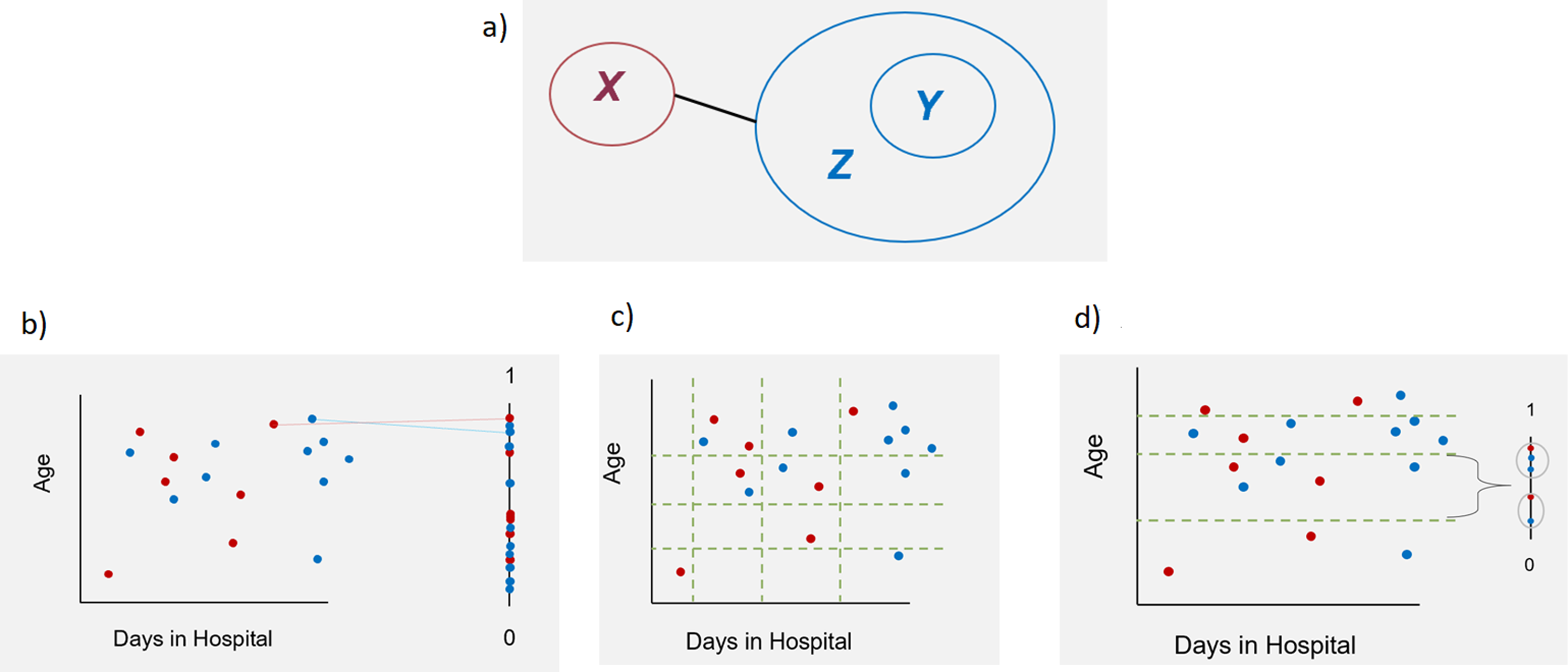

An exact matching, which would ensure exact equal distributions of the matching variables between X and Y, would be ideal to get unbiased results of the analyses. However, this matching procedure often cannot be used in practice because of the strong reduction of group sizes.^7,8 Many different matching procedures with different advantages and disadvantages were developed. One of the methods often used in healthcare research is the propensity score matching (PS). There are different possibilities to compute and use propensity scores.⁹ The easiest way is using a logistic regression model to estimate the probability to belong to group X.⁶ Thereby, the possibly high dimensional dataset is mapped on a one-dimensional scale between 0 and 1.¹⁰ Afterwards, for finding the matching partners the nearest neighbor method is applied using this score (Figure 1(b)). A simple propensity-score matching simulates a randomization.¹¹ The resulting groups can be balanced concerning the mean values but may still differ substantially in the distribution of the different variables.⁷ Therefore, often it makes sense to take the multidimensionality of the data more into account than in simple propensity score matching. In the literature, Coarsened Exact Matching (CEM) and Optimal Full Matching (OFM) are described in this respect.^8,12–17

To perform CEM, classes are formed for each variable to be included in the matching (e.g. age classes, days in hospital classes, etc.) (Figure 1(c)). The width of the classes can be defined by the user. The different classes are considered in every possible combination (e.g. (age class 1, days in hospital class 1); (age class 1, days in hospital class 2)) and the observed values are thus assigned to one of the resulting multidimensional classes. The class sizes can differ, because they are depending on the observed values. Only observations with at least one observation from the measured data X and one observation from the database Z in their class will be considered. Then, exact matching is applied to the classified dataset. For later analyses on the matched dataset, the unclassified (observed) values are used. All analyses have to be weighted after CEM.^8,17,18

OFM is a mixture of matching, subclassification and weighting. It is used less frequently than other methods. Similar to CEM, the dataset is grouped by building one-dimensional or multidimensional classes for the matching variables, whereby each class must consist of at least one measured observation from X and at least one observation from Z. Subsequently, observations within a class are matched to each other by using a distance measure (e.g. the propensity score) and weights are calculated for use in further analyses (Figure 1(d)). The procedure is ‘optimal' since it minimizes the average differences in propensity score between observations from X and Z within a class.¹⁹ One observation from database Z can be matched to one or more observations from the measured dataset X and vice versa.¹⁴

Matching for STROKE OWL

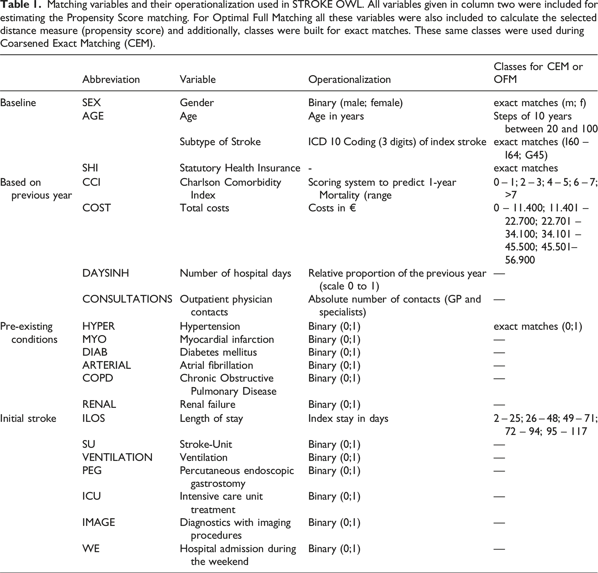
In our case the variable v maps the regions OWL (region 0), Muensterland (region 1) and Sauerland (region 2). The measured dataset X were data from OWL while database Z consisted of data from the two regions Muensterland and Sauerland. Three matching procedures were tested. With regard to the PS, all matching variables (Table 1) were included in the matching without further restrictions. For OFM and CEM, classes were built for some of these variables, in which an exact matching was used. For OFM additionally, all other variables were included to calculate the selected distance measure (propensity score). Analyses were done using R²⁰ (version 4.2.1).

Table 1.

Matching variables and their operationalization used in STROKE OWL. All variables given in column two were included for estimating the Propensity Score matching. For Optimal Full Matching all these variables were also included to calculate the selected distance measure (propensity score) and additionally, classes were built for exact matches. These same classes were used during Coarsened Exact Matching (CEM).

	Abbreviation	Variable	Operationalization	Classes for CEM or OFM
Baseline	SEX	Gender	Binary (male; female)	exact matches (m; f)
	AGE	Age	Age in years	Steps of 10 years between 20 and 100
		Subtype of Stroke	ICD 10 Coding (3 digits) of index stroke	exact matches (I60 – I64; G45)
	SHI	Statutory Health Insurance	-	exact matches
Based on previous year	CCI	Charlson Comorbidity Index	Scoring system to predict 1-year Mortality (range	0 – 1; 2 – 3; 4 – 5; 6 – 7; >7
	COST	Total costs	Costs in €	0 – 11.400; 11.401 – 22.700; 22.701 – 34.100; 34.101 – 45.500; 45.501– 56.900
	DAYSINH	Number of hospital days	Relative proportion of the previous year (scale 0 to 1)	—
	CONSULTATIONS	Outpatient physician contacts	Absolute number of contacts (GP and specialists)	—
Pre-existing conditions	HYPER	Hypertension	Binary (0;1)	exact matches (0;1)
	MYO	Myocardial infarction	Binary (0;1)	—
	DIAB	Diabetes mellitus	Binary (0;1)	—
	ARTERIAL	Atrial fibrillation	Binary (0;1)	—
	COPD	Chronic Obstructive Pulmonary Disease	Binary (0;1)	—
	RENAL	Renal failure	Binary (0;1)	—
Initial stroke	ILOS	Length of stay	Index stay in days	2 – 25; 26 – 48; 49 – 71; 72 – 94; 95 – 117
	SU	Stroke-Unit	Binary (0;1)	—
	VENTILATION	Ventilation	Binary (0;1)	—
	PEG	Percutaneous endoscopic gastrostomy	Binary (0;1)	—
	ICU	Intensive care unit treatment	Binary (0;1)	—
	IMAGE	Diagnostics with imaging procedures	Binary (0;1)	—
	WE	Hospital admission during the weekend	Binary (0;1)	—

Choice of matching procedure

In general, scientists should choose a matching procedure that represents an appropriate compromise between the restrictive maximum claim of exact matching and sufficiently large group sizes. According to Stuart 2010,⁶ it is necessary to evaluate the quality of the matched dataset. There are different methods of evaluating covariate balance.⁶ One possibility presented by Rubin 2001²¹ is to calculate the standardized mean differences for each matching variable.²² If all these differences are less than 0.10 the matching is said to be good in general.²² Due to matching, the dataset is balanced with respect to the matching variables. However, from our point of view this is not necessarily sufficient to generate a good evaluation dataset in health services research. On the one hand this implies that the final dataset already exists, which is not the case when writing the analysis plan. On the other hand, it does not ensure that the chosen matching procedure and covariates are good concerning the possibility of balancing the outcome under the assumption of no intervention effect. We would say, if the matching variables are balanced and a difference in the outcome after the matching occurs, this can be explained in three ways. First, it is possible that an additional variable affecting the outcome (not the region) is missing as matching variable and hence, causes the difference. Second, it is possible that all relevant variables were considered and in fact the region had no influence on the outcome, but the chosen matching procedure was not able to balance the outcome, as one would expect in this case. Third, it is conceivable that the region is responsible for the outcome difference. This third explanation can only be concluded if the other two can be excluded. Hence, differences in the outcome variable could also be attributed to insufficient matching. Nevertheless, in the literature it is often directly assumed that the variable under consideration caused the difference in the outcome when all matching variables are balanced. Therefore, we decided not only checking the balance of the matched dataset after the matching but also checking if the matching procedure and the matching variables are able to balance the outcome at all.

For this purpose, we used the following four-step approach to identify a good matching procedure for STROKE OWL:

A) Identify confounders e.g. using a systematic literature review

B) Check the ability to balance the outcome, when an effect of the region is excluded

C) Check the covariate distributions after matching for the datasets generated in step B

D) Check the remaining group sizes after matching of the datasets generated in step B

Ability to balance the outcome

Suppose all relevant matching variables, which could influence the outcome, have been identified following step A. Hence, the next step was to test the performance of different matching procedures. Assume the following situation: It is found that, after the matching process, all covariates are balanced and there is a difference in outcome. The conclusion that the region has an impact on the outcome is only possible if it has been ensured that the matching worked well. This requires that all relevant variables are really taken into account (ensured by step A) and that the matching also leads to a balance of the outcome, if the region has no effect. To verify this, matching was done within data from the same region. This way region effects were excluded if we assume that each region has a homogeneous outcome in itself. First the procedure was done within data from OWL and afterwards within the regions of Sauerland and Muensterland. As an example, Figure 2 explains the procedure using data from OWL (OWL_data = A_un $\cup$ B_un and A_un $\cap$ B_un = $\emptyset$ ). 500 random people were sampled to generate dataset A_un. Afterwards matching was performed between A_un and B_un, which lead to the matched datasets A_m and B_m. The standardized mean differences of the outcome were calculated for the unmatched and matched dataset. This procedure was repeated 100 times and finally the means of the standardized mean differences were computed. The ratio between these means was used as an indicator how well the matching under consideration was able to balance the outcome. The larger this value, the better the matching can compensate for the differences in the outcome. Hence, large values indicate that the matching procedure works well on the dataset concerning the ability to balance the outcome, when this can be expected. More detailed explanations are given in the Appendix A2. When the whole procedure is repeated on the same dataset and the results show huge differences, it is advisable to (greatly) increase the number of data sets drawn (A_un), as it can be assumed that the results will converge with a larger number of draws due to the law of large numbers.

Figure 2.

Ability to balance the outcome: All observations are from the same region, hence matching between A_un and B_un excludes regional effects and therefore a lower standardized mean difference of the outcome can be expected in the matched dataset, if a matching procedure worked well and all relevantmatching variables are considered.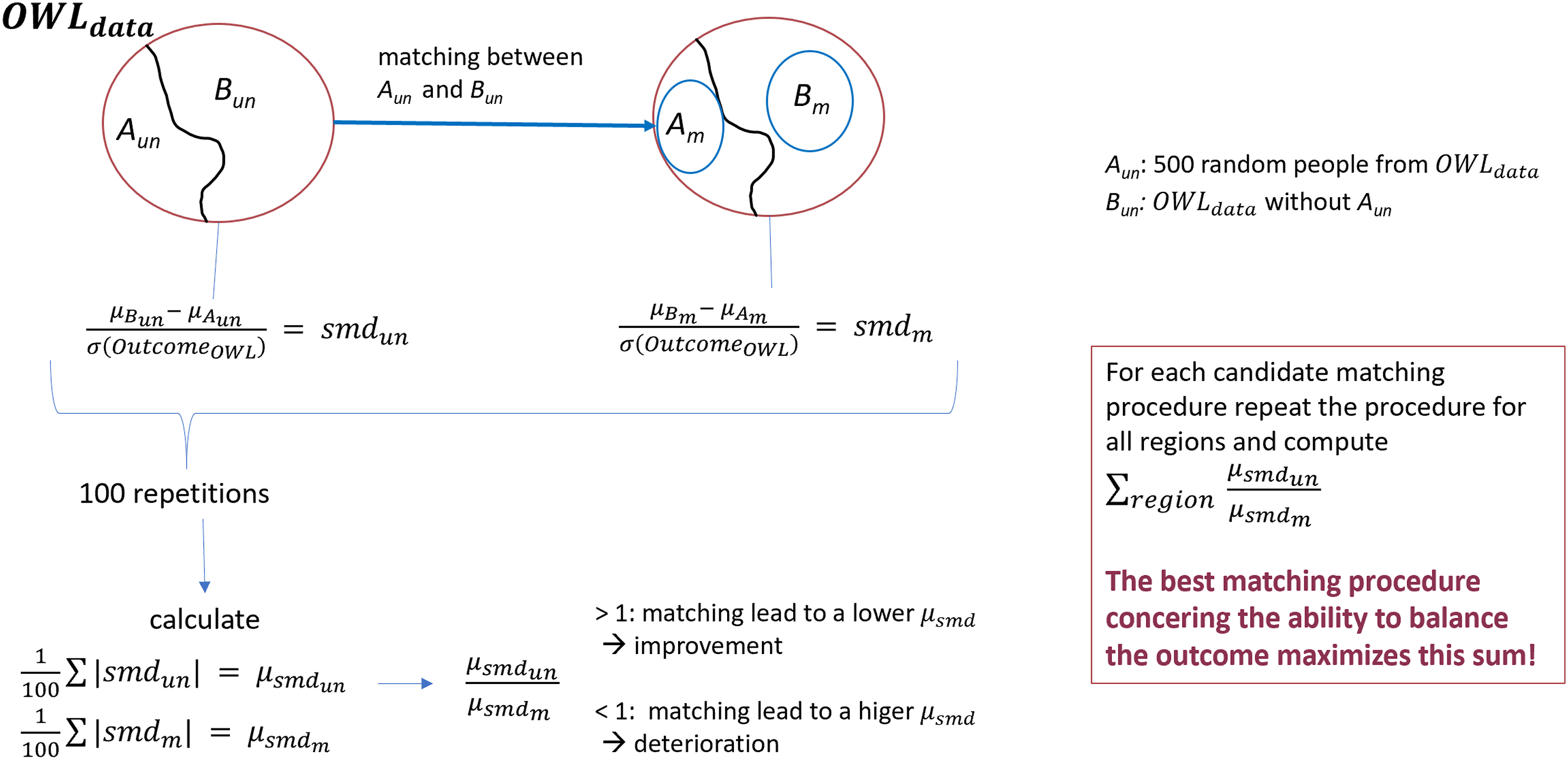

Covariate balance and group size after matching

To obtain a comprehensive picture of the matching procedure under consideration, the distributions of the covariates in the different datasets A_m and B_m were calculated and the difference of densities between each pair of A_m and B_m for continuous variables were inspected.²² Since many datasets were generated during the described procedure, it will be difficult to visualize all these density curve pairs. We plotted one line for each pair of matched datasets presenting the difference of the density curves. The closer a line is to zero, the more similar the distributions of the covariate under consideration between the datasets A_m and B_m. For ordinal or nominal variables, a visualization using cumulative bar charts was used. Moreover, the remaining group sizes needed to be assessed. This was done by looking at the distribution of losses of observations across the datasets A_m.

Results

Identify confounders

At first all relevant matching variables had to be identified. Hence, a systematic literature search was conducted to define relevant factors influencing stroke recurrences (for details see Aufenberg et al. 2024²³). Therefore, the MEDLINE database was systematically screened via Pubmed for studies with a population consisting of patients with stroke or TIA (≥18 years of age and representing the general stroke population). Predictors have been identified as relevant for the matching, if they have been mentioned in at least two independent publications and, in addition, if they were reported as significant in at least one of these publications.

Ability to balance the outcome

Table 2 shows the ability to balance the outcome following step B. It turned out that CEM was able to create datasets with standardized mean differences of stroke recurrences of 0 after the matching in each region. This is the best value achievable since there is no difference concerning stroke recurrences between the subgroups any longer. OFM led to a value of 2.3419 when summing over the quotients of the standardized mean differences, while PS achieved a value of 2.5616. Hence the maximum of this value is said to indicate the best matching procedure, the PS worked better than OFM. Nevertheless, the quotient of the mean of the standardized mean differences for OFM and PS was always less than 1, which indicates a deterioration compared to the unmatched dataset. To give a more detailed impression of how the matching procedures worked, the distributions of the standardized mean differences for all three tested methods and the unmatched datasets stratified by the regions are shown in Figure 3(a). It should be mentioned that CEM led to 0 every time. OFM and PS showed larger boxes and ranges than the unmatched datasets and hence confirmed the impression that the procedures more likely led to deteriorations concerning the outcome balance rather than improvements. Figure 3(b) visualizes the distributions of the quotients for OFM and PS. The boxes are close to zero and look similar. Nevertheless, for OFM, some huge outliers can be identified.

Table 2.

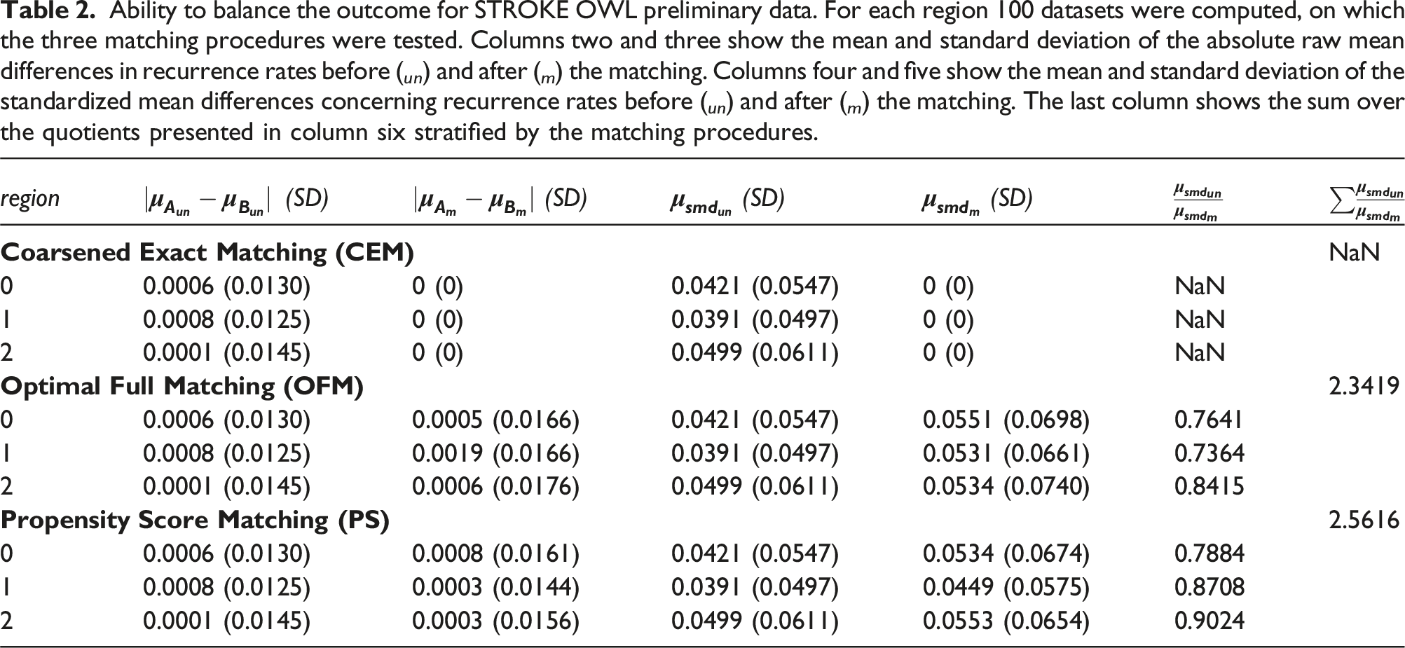
Ability to balance the outcome for STROKE OWL preliminary data. For each region 100 datasets were computed, on which the three matching procedures were tested. Columns two and three show the mean and standard deviation of the absolute raw mean differences in recurrence rates before (_un) and after (_m) the matching. Columns four and five show the mean and standard deviation of the standardized mean differences concerning recurrence rates before (_un) and after (_m) the matching. The last column shows the sum over the quotients presented in column six stratified by the matching procedures.

region	$\| μ_{A_{u n}} - μ_{B_{u n}} \|$ (SD)	$\| μ_{A_{m}} - μ_{B_{m}} \|$ (SD)	$μ_{{s m d}_{u n}}$ (SD)	$μ_{{s m d}_{m}}$ (SD)	$\frac{μ_{{s m d}_{u n}}}{μ_{{s m d}_{m}}}$	$\sum \frac{μ_{{s m d}_{u n}}}{μ_{{s m d}_{m}}}$
Coarsened Exact Matching (CEM)						NaN
0	0.0006 (0.0130)	0 (0)	0.0421 (0.0547)	0 (0)	NaN
1	0.0008 (0.0125)	0 (0)	0.0391 (0.0497)	0 (0)	NaN
2	0.0001 (0.0145)	0 (0)	0.0499 (0.0611)	0 (0)	NaN
Optimal Full Matching (OFM)						2.3419
0	0.0006 (0.0130)	0.0005 (0.0166)	0.0421 (0.0547)	0.0551 (0.0698)	0.7641
1	0.0008 (0.0125)	0.0019 (0.0166)	0.0391 (0.0497)	0.0531 (0.0661)	0.7364
2	0.0001 (0.0145)	0.0006 (0.0176)	0.0499 (0.0611)	0.0534 (0.0740)	0.8415
Propensity Score Matching (PS)						2.5616
0	0.0006 (0.0130)	0.0008 (0.0161)	0.0421 (0.0547)	0.0534 (0.0674)	0.7884
1	0.0008 (0.0125)	0.0003 (0.0144)	0.0391 (0.0497)	0.0449 (0.0575)	0.8708
2	0.0001 (0.0145)	0.0003 (0.0156)	0.0499 (0.0611)	0.0553 (0.0654)	0.9024

Figure 3.

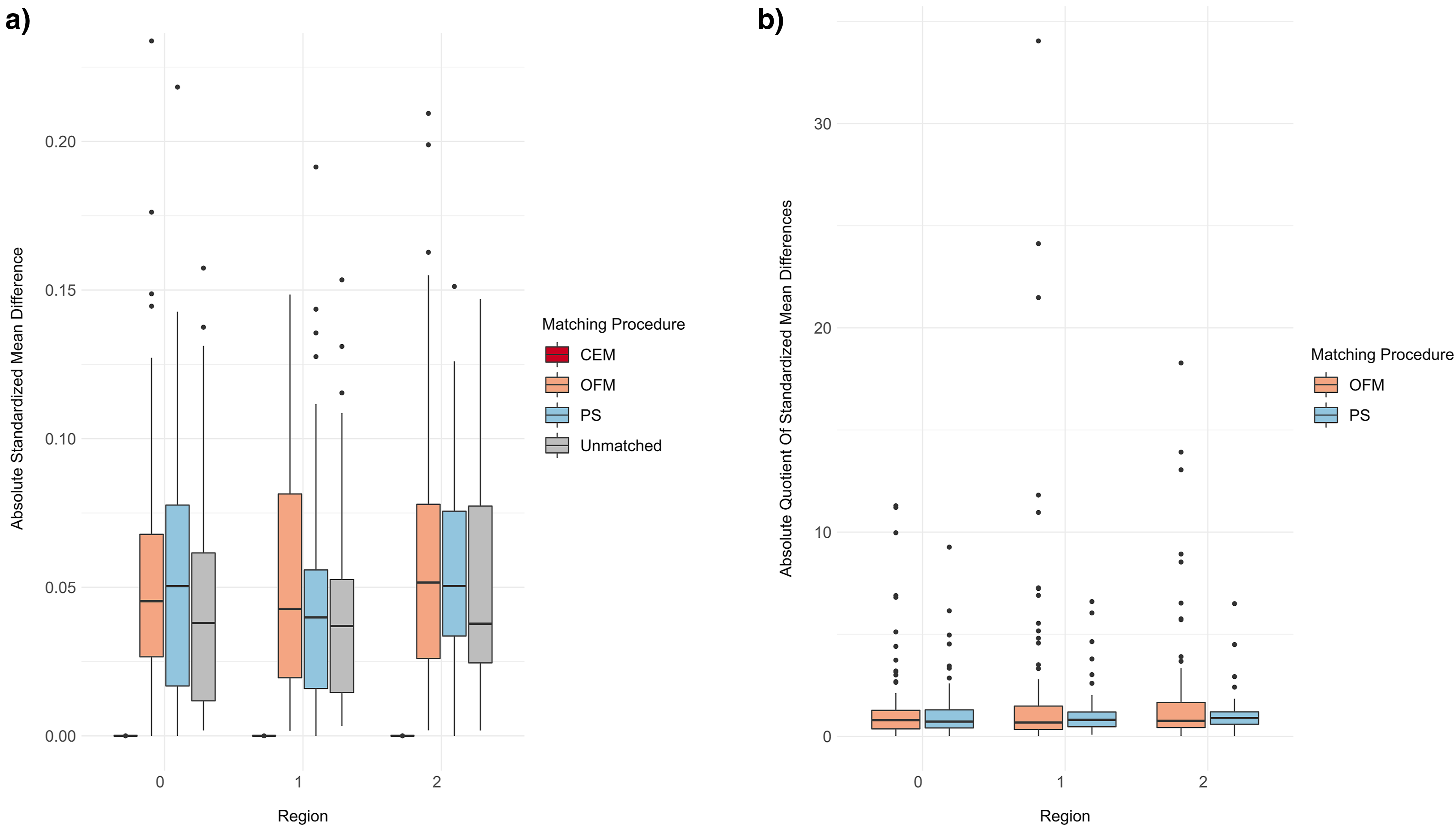
(a): Distribution of the absolute standardized mean differences for each matching procedure stratified by regions. (b): Distribution of the quotients of absolute standardized mean differences between unmatched and matched datasets for OFM and PS stratified by regions.

Covariate distributions

The covariate distributions (step C) cannot be presented in detail for each combination of region and matching procedure. The distribution of the 300 absolute standardized mean differences for each procedure and the unmatched case is shown in Figure 4. It can be seen that all matching procedures were able to achieve an improvement over the unmatched data for continuous variables. It should be noted that only a few relevant deviations (>10%) occurred in the unmatched datasets. For binary outcomes, PS worked better than CEM and OFM. The last two lead to larger boxes and higher medians than the unmatched dataset.

Figure 4.

(a) Distribution of absolute standardized mean differences for continuous/ordinal matching variables stratified by matching procedures. (b) Distribution of absolute standardized mean differences for binary matching variables stratified by matching procedures. Abbreviations see Table 1.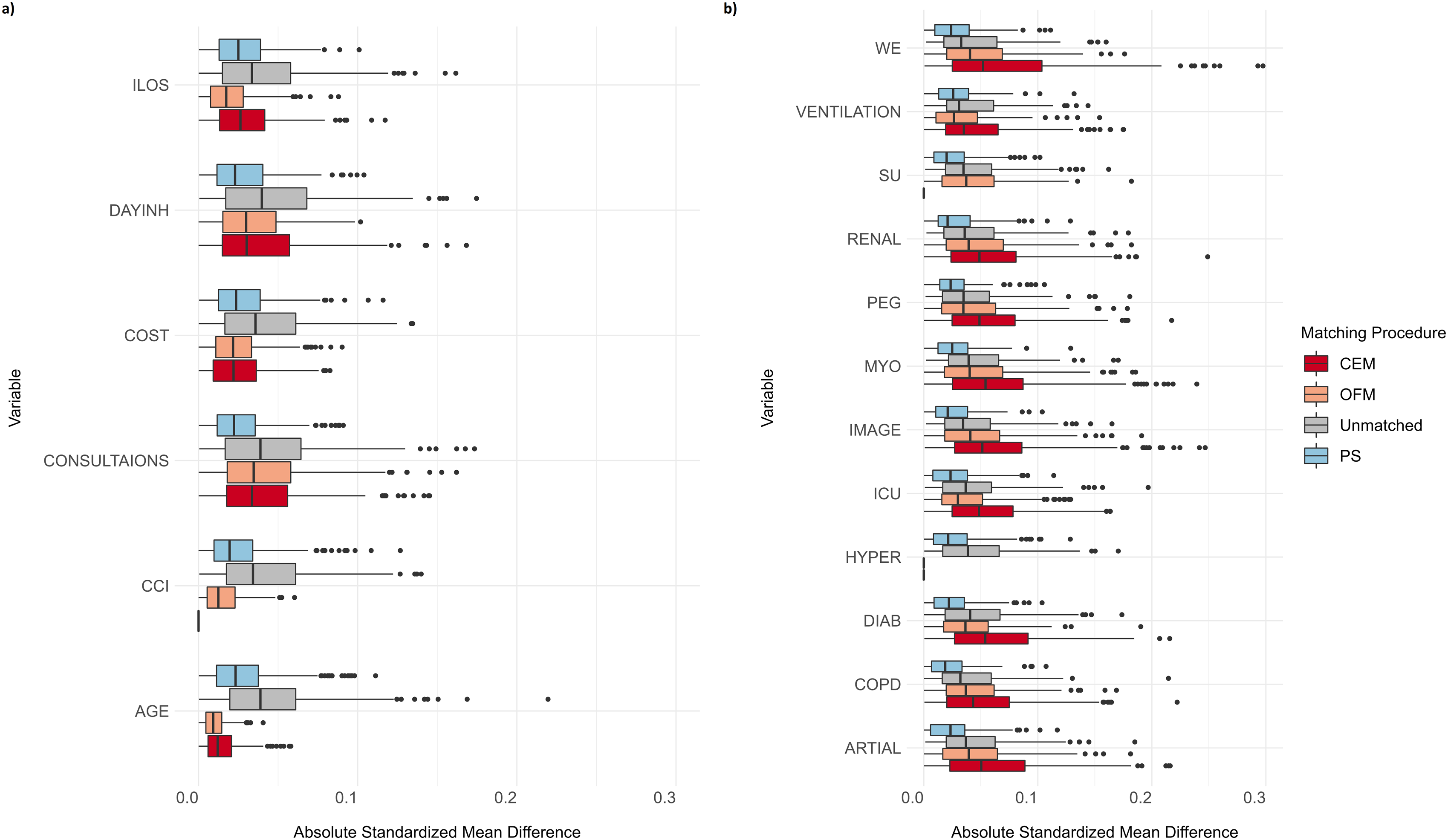

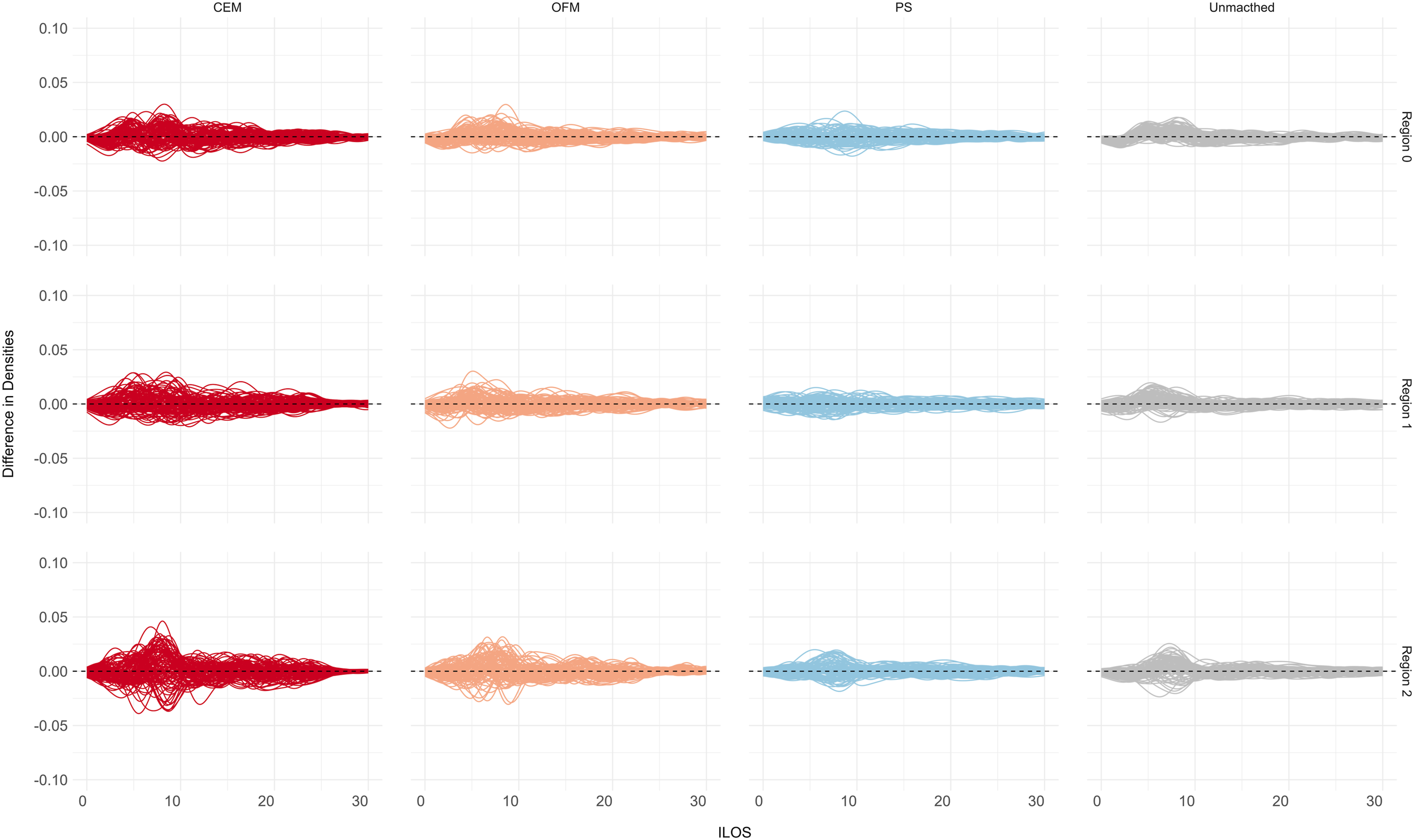
For ordinal or nominal variables, additional cumulative bar plots can help to get an impression of the whole distributions in the different datasets. As an example, such a plot was created for the ordinal covariate ‘charlson comorbidity index’ (CCI) (Figure 5). Only the 10 most differing datasets before the matching were chosen to be presented as an excerpt. In this case, CEM always balanced the datasets completely, while for OFM and PS no major differences can be detected. For continuous variables, a closer look at the differences of the density curves can help (Figure 6). As an example, the covariate ‘initial stay in hospital’ (ILOS) in days is presented. This indicates that the PS and OFM partly delivered better results than CEM. The differences seen for CEM are still lower than 0.05 and this holds for all other covariates as well.

Figure 5.

Cumulative barplots for the matching variable ‘Charlston comborbidity index’ (CCI).

Figure 6.

Difference of densities for the matching variable ‘initial length of stay’ (ILOS).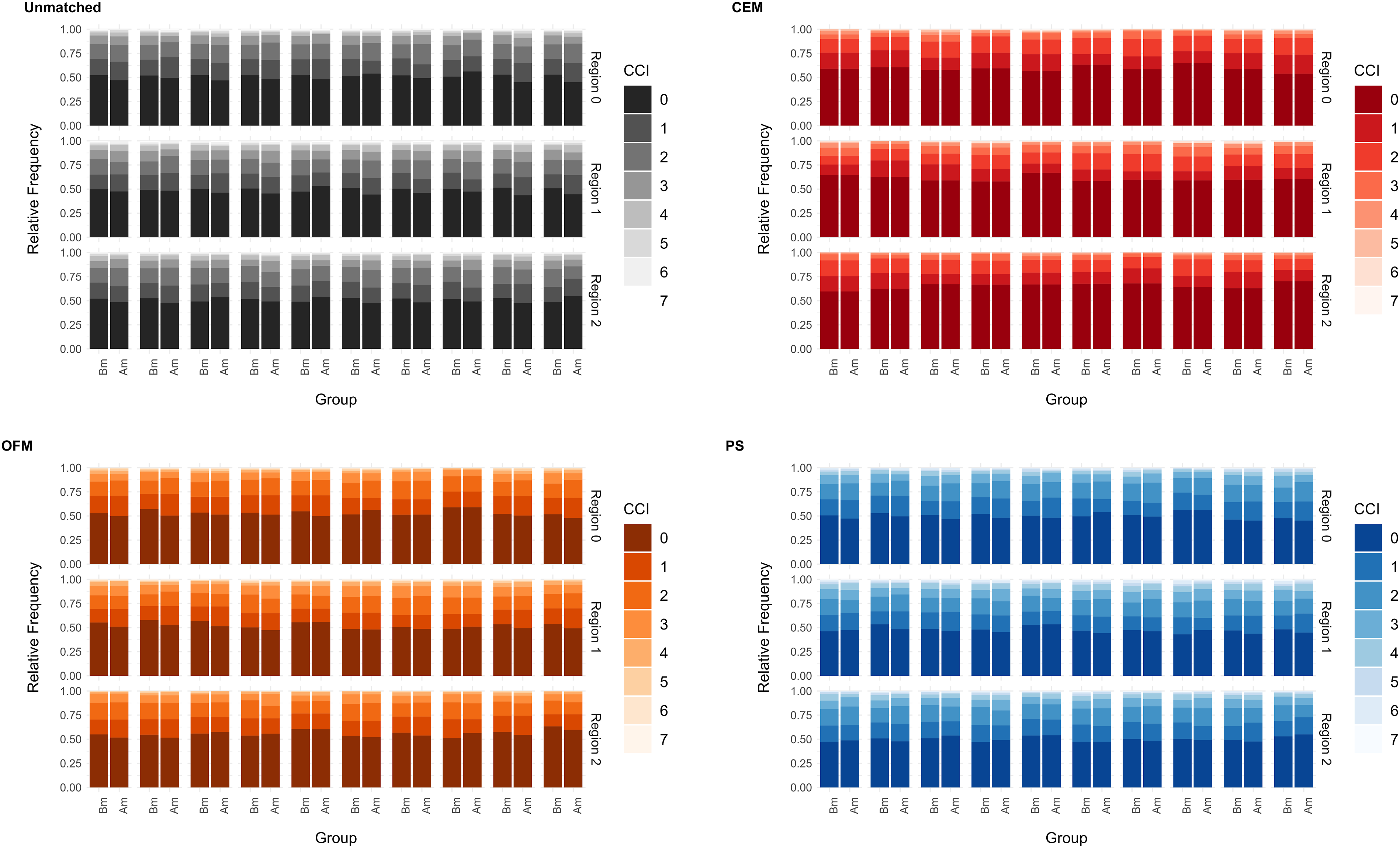

Group sizes

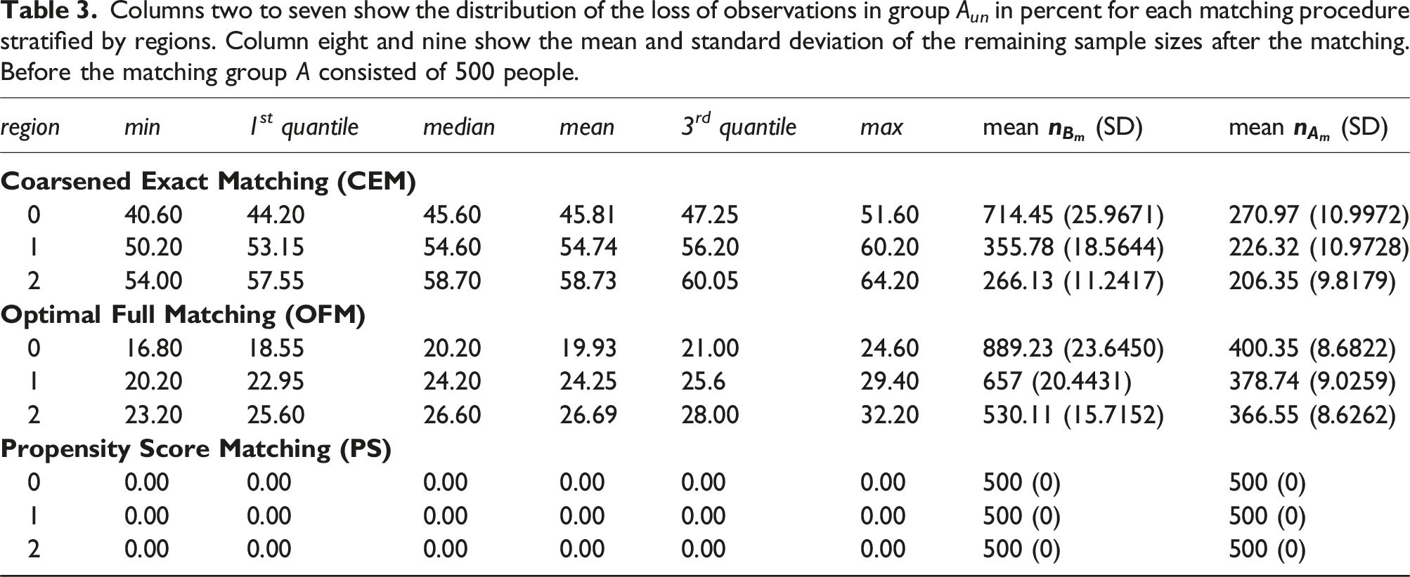
When using CEM on average more than 50% of the observations from the measured group were lost (Table 3). In case of OFM the loss was 24% on average while for PS a 1:1 Matching was used and hence all observations were retained.

Table 3.

Columns two to seven show the distribution of the loss of observations in group A_un in percent for each matching procedure stratified by regions. Column eight and nine show the mean and standard deviation of the remaining sample sizes after the matching. Before the matching group A consisted of 500 people.

region	min	1 ^st quantile	median	mean	3 ^rd quantile	max	mean $n_{B_{m}}$ (SD)	mean $n_{A_{m}}$ (SD)
Coarsened Exact Matching (CEM)
0	40.60	44.20	45.60	45.81	47.25	51.60	714.45 (25.9671)	270.97 (10.9972)
1	50.20	53.15	54.60	54.74	56.20	60.20	355.78 (18.5644)	226.32 (10.9728)
2	54.00	57.55	58.70	58.73	60.05	64.20	266.13 (11.2417)	206.35 (9.8179)
Optimal Full Matching (OFM)
0	16.80	18.55	20.20	19.93	21.00	24.60	889.23 (23.6450)	400.35 (8.6822)
1	20.20	22.95	24.20	24.25	25.6	29.40	657 (20.4431)	378.74 (9.0259)
2	23.20	25.60	26.60	26.69	28.00	32.20	530.11 (15.7152)	366.55 (8.6262)
Propensity Score Matching (PS)
0	0.00	0.00	0.00	0.00	0.00	0.00	500 (0)	500 (0)
1	0.00	0.00	0.00	0.00	0.00	0.00	500 (0)	500 (0)
2	0.00	0.00	0.00	0.00	0.00	0.00	500 (0)	500 (0)

Discussion

The objective of this article was to present a novel approach for comparing matching procedures before final data analyses take place. Therefore, the selection approach of a suitable matching procedure for the STROKE OWL study was disclosed. A four-step approach was introduced. All in all, the analyses showed that it is challenging to identify a suitbale matching procedure, since the results of the different balance and group size checks can be heterogeneous. However, since there is little described in the literature about how matching procedures are selected prior the final analyses, this article provides initial guidance. Another approach for the selection of a suitable procedure is given by Markoulidakis et al. 2023.²⁴

Discussion of STROKE OWL matching

The analyses showed that CEM was able to compensate for differences in the outcome very well. In terms of balancing the (other) covariates, the method was not relevantly inferior to OFM and the PS concerning continuous or ordinal variables. Therefore, it would have been obvious to use CEM matching for STROKE OWL. However, due to the massive loss of observations, this was not possible in practice. Furthermore, it should be stated that CEM is able to balance small numbers of covariates very well but if there are more variables to balance the procedure might not be useful.²⁵ OFM and the PS both showed weaknesses in the ability to achieve a balance with respect to the outcome. It should be noted, that the absolute mean differences were already small before matching (mean always less than 1%). Hence, improvements are very difficult to show. Therefore, the results of step B should not be overinterpreted. Outliers in the boxplot for quotients of the standardized mean differences indicate, that in some cases the procedures worked very well. OFM was slightly better at balancing the standardized mean differences of continuous covariates, while PS worked better for binary variables. For the STROKE OWL study, a dropout rate of 25 % of the intervention participants was calculated and thus the loss of some observations did not seem to be a problem for the use of the OFM. Additionally, the data quality check showed strongly limited comparability of the data between the different SHIs. This resulted in the need for exact matches for SHI as well as for some other variables. Overall, OFM was chosen as the matching method for STROKE OWL because it represented the best compromise of the requirements.

Discussion of the matching procedures

Some of the characteristics of the three tested matching procedures and limitations of the presented research should be discussed. CEM is known to lead to highly balanced datasets, although a reduction in the size of comparison groups can be expected.⁸ The results of the case study show that the balance is expectable only regarding to the actually used covariates and within the used classes. However, differences can arise when considered over the entire dataset. For binary variables, it is shown that CEM worked worse than OFM and PS. Unless these variables can be considered exactly in the matching, CEM cannot improve the balance compared to the unmatched datasets. Using binary variables as matching variables in CEM might lead to problems, since the remaining sizes of comparison groups can largely be reduced if the variable is highly imbalanced between the unmatched datasets. Other procedures like PS or OFM are able to control for binary variables without pruning observations as much. Because studies in health services research are expensive and usually assume a dropout rate of 20 to 25%,^26,27 practical applicability of CEM in this scientific field in general is doubtful. In general it should be kept in mind, that dropping observations from the treatment group during the matching process leads to changes in the estimated outcome effect.²⁸

During the analyses OFM and PS showed only minor differences. PS was used as the distance measure in OFM. Other distance measures are possible as well,¹⁶ e.g. mahalanobis distance or euclidean distance. Mahalanobis distance is known to work well for less than eight normally distributed covariates.^13,29 Using one of these measures during OFM might lead to other results than in the presented case study. The use of a 1:1 propensity score matching enables the inclusion of all observations in the matched dataset. Without further restrictions, it is not possible to control exactly for variables. However, due to poor data quality or use of different data sources to generate the comparison group Y, exact balance may be necessary. In such cases, the unrestricted use of the propensity score is not recommended. Nevertheless, it should be mentioned that there are already considerations and recommendations regarding the reduction of bias when applying the propensity score in quasi-experimental studies.^30,31 All in all there is a wide range of matching procedures that can be used.^28,32,33 However, there are alternatives to matching in general, such as subclassification, weighting or stratification^6,33–38

Limitations

The matching variables were determined using a systematic literature review.²³ No further reduction of the identified variables had been done. It is a limitation that this procedure can lead to overfitting in the later models. For the analyses, it is therefore important to check overfitting of the models and, if necessary, to avoid it by using regularization approaches (e.g. lasso or factor analysis) to reduce the number of covariates in the models.

The aim of our step B (the ability to balance the outcome) is testing whether the matching procedure under consideration is able to balance the outcome within one region. This assumes that all relevant matching variables have been identified, used as covariates and have been balanced after the matching. In practical use, however, this can be problematic, since further, unconsidered variables must always be expected. Hence, this procedure can lead to biased results when these assumptions are not full field. The conclusion, that an outcome balance has to be achieved while matching within a region can be wrong. In addition, there may be ambiguities if the tested matching procedure leads to different results within different regions. At this point, it is not defined how to proceed if a matching procedure works in one region but not in another one. However, when different regions are rather different regarding the covariate distributions, a procedure improving a balance within one of these groups might not ensure the balancing of variables across groups.

The propensity score distributions of the unmatched datasets of step B have been very similar and our analyses led to low standardized mean differences even before matching was done. On the one hand, this confirms that each region has homogeneous recurrence rates in itself, on the other hand, improvements are more difficult to show in these cases. Hence, it might be useful to generate datasets with higher differences concerning the outcome standardized mean difference. Medical studies are particularly vulnerable to self-selection bias in the measured datasets, when individuals who participate in a study differ in relevant clinical characteristics from those who do not. Therefore, it is important to check whether the matching procedure leads to good results for such cases.

The balance of the covariates is also investigated in many other studies.^6,22 It should be noted that a complete consideration of the distributions is not given in most cases. In the literature, it is recommended to consider the standardized mean differences.²¹ The possibility of representing the entire distributions and/or their differences should be tested to get a better overall picture of how different matching procedures work and to identify their advantages and disadvantages on the underlying datasets. (e.g. differences in density curves). Alternatives for checking covariate balances were developed, for example based on machine learning³⁹ or using simulation studies.⁹

Conclusion

Matching, weighting and subclassification can be useful statistical techniques in the context of evaluating real world data and quasi-experimental studies, which, properly applied, can increase the trustworthiness of results.³² In summary, it can be said that the best choice of a procedure always depends on a number of varying factors. On the one hand, researches have to decide which aspects of the matched dataset are most suitable (number of remaining cases vs balance) and, on the other hand, data quality has an impact on which procedure can be used. Low data quality might lead to the need for exact matches for some variables. In all cases, it should be kept in mind that it is not sufficient to check the balances of covariates after matching to ensure the quality of reported results on matched datasets, since it is possible that improperly chosen matching procedures or missing matching variables lead to wrong conclusions. We have disclosed our procedure for selecting the matching method and stayed independent of the final study data set by using preliminary data. More research will be needed to generate an objective rule to choose the most appropriate method for public health or health services research before the final analyses are conducted.

Supplemental Material

Supplemental Material - Identification of a suitable matching procedure in health services research: Insights into a study for stroke patients

Supplemental Material for Identification of a suitable matching procedure in health services research: Insights into a study for stroke patients by Svenja Elkenkamp, Juliane Düvel, Daniel Gensorowsky and Wolfgang Greiner in Research Methods in Medicine & Health Sciences

Footnotes

Acknowledgments

We thank John Grosser and Christiane Fuchs for critically proofreading the manuscript. The project STROKE OWL was supported by innovation funds of the Federal Joint Committee (G-BA) (No.: 01NVF17025).

Authors’ contributions

SE: conceptualization, formal analysis, methodology, project administration, visualization, writing and reviewing the original draft. JD: conceptualization, formal analysis, methodology, project administration, writing and reviewing the original draft. DG: conceptualization, methodology, project administration, reviewing the original draft. WG: funding acquisition, supervision, reviewing the original draft.

Declaration of conflicting interests

The author(s) declared no potential conflicts of interest with respect to the research, authorship, and/or publication of this article.

Funding

The author(s) disclosed receipt of the following financial support for the research, authorship, and/or publication of this article: This work was supported by the Innovation funds of the Federal Joint Committee (G-BA); No.: 01NVF17025.

Trial registration

The STROKE OWL study was registered on German Clinical Trials Register, retrospective registration on 21/09/2022 (DRKS00030297).

Ethical statement

ORCID iD

Svenja Elkenkamp

Supplemental material

Supplemental material for this article is available online.

References

Liu

Panagiotakos

. Real-world data: a brief review of the methods, applications, challenges and opportunities. BMC Med Res Methodol 2022; 22: 287.

Eberwein

Ham

Lalonde

. The impact of being offered and receiving classroom training on the employment histories of disadvantaged women: evidence from experimental data. Rev Econ Stud 1997; 64: 655–682.

Heinz

Wendel-Garcia

Held

. Impact of the matching algorithm on the treatment effect estimate: a neutral comparison study. Biom J 2024; 66: e2100292.

Duevel

Elkenkamp

Gensorowsky

, et al. A case management intervention in stroke care: evaluation of a quasi-experimental study. Z Evid Fortbild Qual Gesundhwes 2024; 187: 69–78.

Duevel

Gruhn

Grosser

, et al. Secondary prevention via case managers in stroke patients: a cost-effectiveness analysis of claims data from German statutory health insurance providers. Healthcare 2024; 12: 1157.

Stuart

. Matching methods for causal inference: a review and a look forward. Stat Sci 2010; 25: 1–21.

King

Nielsen

. Why propensity scores should not Be used for matching. Polit Anal 2019; 27: 435–454.

Iacus

King

Porro

. Causal inference without balance checking: coarsened exact matching. Polit Anal 2012; 20: 1–24.

Franklin

Eddings

Austin

, et al. Comparing the performance of propensity score methods in healthcare database studies with rare outcomes. Stat Med 2017; 36: 1946–1963.

10.

Rosenbaum

Rubin

. The central role of the propensity score in observational studies for causal effects. Biometrika 1983; 70: 41–55.

11.

Austin

. An introduction to propensity score methods for reducing the effects of confounding in observational studies. Multivariate Behav Res 2011; 46: 399–424.

12.

Ripollone

Huybrechts

Rothman

, et al. Evaluating the utility of coarsened exact matching for pharmacoepidemiology using real and simulated claims data. Am J Epidemiol 2020; 189: 613–622.

13.

Rosenbaum

. Comparison of multivariate matching methods: structures, distances, and algorithms. J Comput Graph Stat 1993; 2: 405–420.

14.

Hansen

. Full matching in an observational study of coaching for the SAT. J Am Stat Assoc 2004; 99: 609–618.

15.

Rosenbaum

. Optimal matching for observational studies. J Am Stat Assoc 1989; 84: 1024.

16.

Stuart

Green

. Using full matching to estimate causal effects in nonexperimental studies: examining the relationship between adolescent marijuana use and adult outcomes. Dev Psychol 2008; 44: 395–406.

17.

Iacus

King

Porro

. Cem software for coarsened exact matching. J Stat Software 2009; 30.

18.

Iacus

King

Porro

. A theory of statistical inference for matching methods in causal research. Polit Anal 2019; 27: 46–68.

19.

Austin

Stuart

. The performance of inverse probability of treatment weighting and full matching on the propensity score in the presence of model misspecification when estimating the effect of treatment on survival outcomes. Stat Methods Med Res 2017; 26: 1654–1670.

20.

R Core Team . R: a language and environment for statistical. Vienna: Foundation for Statistical Computing, 2022.

21.

Rubin

. Using Propensity Scores to Help Design Observational Studies: Application to the Tobacco Litigation. Health Serv Outcome Res Methodol. 2001; 2: 169–188.

22.

Zhang

Kim

Lonjon

, et al. Balance diagnostics after propensity score matching. Ann Transl Med 2019; 7: 16.

23.

Aufenberg

Düvel

Morthorst

, et al. Prädiktoren für die Folgen eines Schlaganfalls: eine systematische Literaturübersicht für GKV-Routinedatenanalysen. Gesundheitsökonomie & Qualitätsmanagement. 2024.

24.

Markoulidakis

Taiyari

Holmans

, et al. A tutorial comparing different covariate balancing methods with an application evaluating the causal effects of substance use treatment programs for adolescents. Health Serv Outcome Res Methodol 2023; 23: 115–148.

25.

Black

Lalkiya

Lerner

. The trouble with coarsened exact matching. Northwestern Law & Econ Research Paper Forthcoming. (2020, October 6). doi:10.2139/ssrn.3694749, https://ssrn.com/abstract=3694749.

26.

Dixon

Linardon

. A systematic review and meta-analysis of dropout rates from dialectical behaviour therapy in randomized controlled trials. Cognit Behav Ther 2020; 49: 181–196.

27.

Dettori

Norvell

Skelly

, et al. Heterogeneity of treatment effects: from “How to treat” to “Whom to treat”. Evid Base Spine Care J 2011; 2: 7–10.

28.

Imai

King

, et al. Matching as nonparametric preprocessing for reducing model dependence in parametric causal inference. Polit Anal 2007; 15: 199–236.

29.

Zhao

. Using matching to estimate treatment effects: data requirements, matching metrics, and Monte Carlo evidence. Rev Econ Stat 2004; 86: 91–107.

30.

Groenwold

RHH

de Vries

de Boer

, et al. Balance measures for propensity score methods: a clinical example on beta-agonist use and the risk of myocardial infarction. Pharmacoepidemiol Drug Saf 2011; 20: 1130–1137.

31.

Stuart

Lee

Leacy

. Prognostic score-based balance measures can be a useful diagnostic for propensity score methods in comparative effectiveness research. J Clin Epidemiol 2013; 66: S84–S90.

32.

Greifer

Stuart

. Matching methods for confounder adjustment: an addition to the epidemiologist's toolbox. Epidemiol Rev 2022; 43: 118–129.

33.

Rosenbaum

Rubin

. Constructing a control group using multivariate matched sampling methods that incorporate the propensity score. Am Statistician 1985; 39: 33–38.

34.

Cochran

. The effectiveness of adjustment by subclassification in removing bias in observational studies. Biometrics 1968; 24: 295–313.

35.

Ben-Michael

Keele

. Using balancing weights to target the treatment effect on the treated when overlap is poor. Epidemiology 2023; 34: 637–644.

36.

Chesnaye

Stel

Tripepi

, et al. An introduction to inverse probability of treatment weighting in observational research. Clin Kidney J 2022; 15: 14–20.

37.

Huling

Mak

. Energy balancing of covariate distributions. J Causal Inference 2024; 12.

38.

Huling

Greifer

Chen

. Independence weights for causal inference with continuous treatments. J Am Stat Assoc 2024; 119: 1657–1670.

39.

Linden

Yarnold

. Using machine learning to assess covariate balance in matching studies. J Eval Clin Pract 2016; 22: 844–850.

Supplementary Material

Please find the following supplemental material available below.

For Open Access articles published under a Creative Commons License, all supplemental material carries the same license as the article it is associated with.

For non-Open Access articles published, all supplemental material carries a non-exclusive license, and permission requests for re-use of supplemental material or any part of supplemental material shall be sent directly to the copyright owner as specified in the copyright notice associated with the article.

0.00 MB

0.24 MB