Approximately unbiased estimators of the inverse variance from sample summary statistics

Abstract

Background

In meta-analysis, researchers often pool the results from a set of similar studies. A number of studies, however, often tend to report only the minimum and maximum values, median, and/or the first and third quartiles. Recently, many methods have been discussed for estimating the mean and standard deviation from those sample summaries. However, these methods may provide a substantially biased estimate of the inverse variance that is needed for the meta-analysis.

Research Design

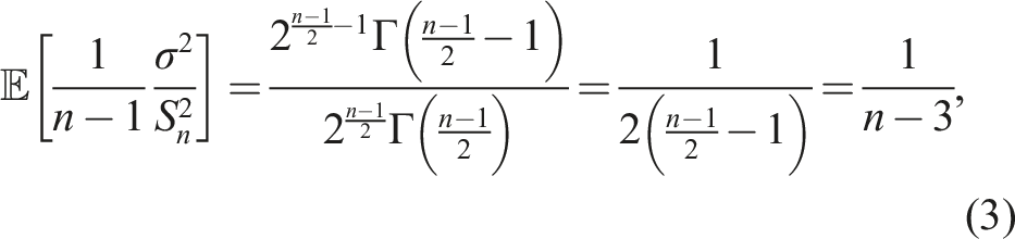
We use Basu’s theorem to derive unbiased estimators for σ⁻² from the most commonly used sample summaries from the normal distribution. While there are no closed formulas for these estimators, we use simulations to obtain simple approximations for the estimators.

Results

The proposed approximate estimators still show a little to no bias for normally distributed data and generally show smaller bias than the usual methods even for some non-normal distributions. The proposed estimators have lower mean squared error.

Conclusions

The proposed estimators are recommended for the purpose of obtaining inverse-variance weights, particularly in the context of meta-analyses.

Introduction

When one wishes to combine data from multiple independent studies, the sample mean and sample standard deviation are the essential quantities for the meta-analysis. ¹ Some studies do not report either the mean or the standard deviation and report only the five-figure summary (including the sample median, the first and third quartiles, and the minimum and maximum values). Moreover, even the five-figure summary may not be fully reported; see, for example, Thatcher et al., ² where only the median and range were reported or Monaco et al. ³ where only the median and the quartiles were reported. Rather than discarding the studies that do not report the sample mean and standard deviation directly, one can try to estimate these quantities from the reported summaries. While the work on this problem can be traced back all the way to Tippett, ⁴ the interest in the systematic research of the estimators resurfaced in Hozo et al. ⁵ and a significant body of literature soon followed;^6–11 see also Weir et al. ¹² and Walter et al. ¹³ where various methods have been discussed and compared.

Typically, three scenarios are investigated depending on the summaries being reported in addition to a sample size:

1. {a, m, b; n},

2. {q₁, m, q₃; n}, or

3. {a, q1, m, q3, b},

where a is the minimum, q₁ is the first quartile, m is the median, q₃ is the third quartile, b is the maximum and n is the sample size.

Walter et al. ¹³ showed that a naïve method for estimating σ⁻² in Scenario 1 by estimating σ first and then raising that estimate to power −2 can result in substantial bias, particularly for small samples. This is true even for the state-of-the-art methods presented in Shi et al. ¹⁴ and Balakrishnan et al.; ¹⁵ see Figure 1. Therefore, Walter et al. ¹³ used a Taylor series approximation to provide a better estimate for σ⁻² when only the sample range is available. They showed that the approximation by the polynomial of fourth degree yields good results even for small sample sizes.

Figure 1.

Bias and mean square error (MSE) of estimating σ⁻² by first estimating σ using the best methods for the appropriate scenario from Shi et al. ¹⁴ and Balakrishnan et al. ¹⁵ and then raising the estimate to power −2. Results from 10⁵ simulations for data from N(0, 1) are shown; however, the bias and MSE is the same regardless of the mean and the variance of the normal distribution. (a) Bias. (b) MSE.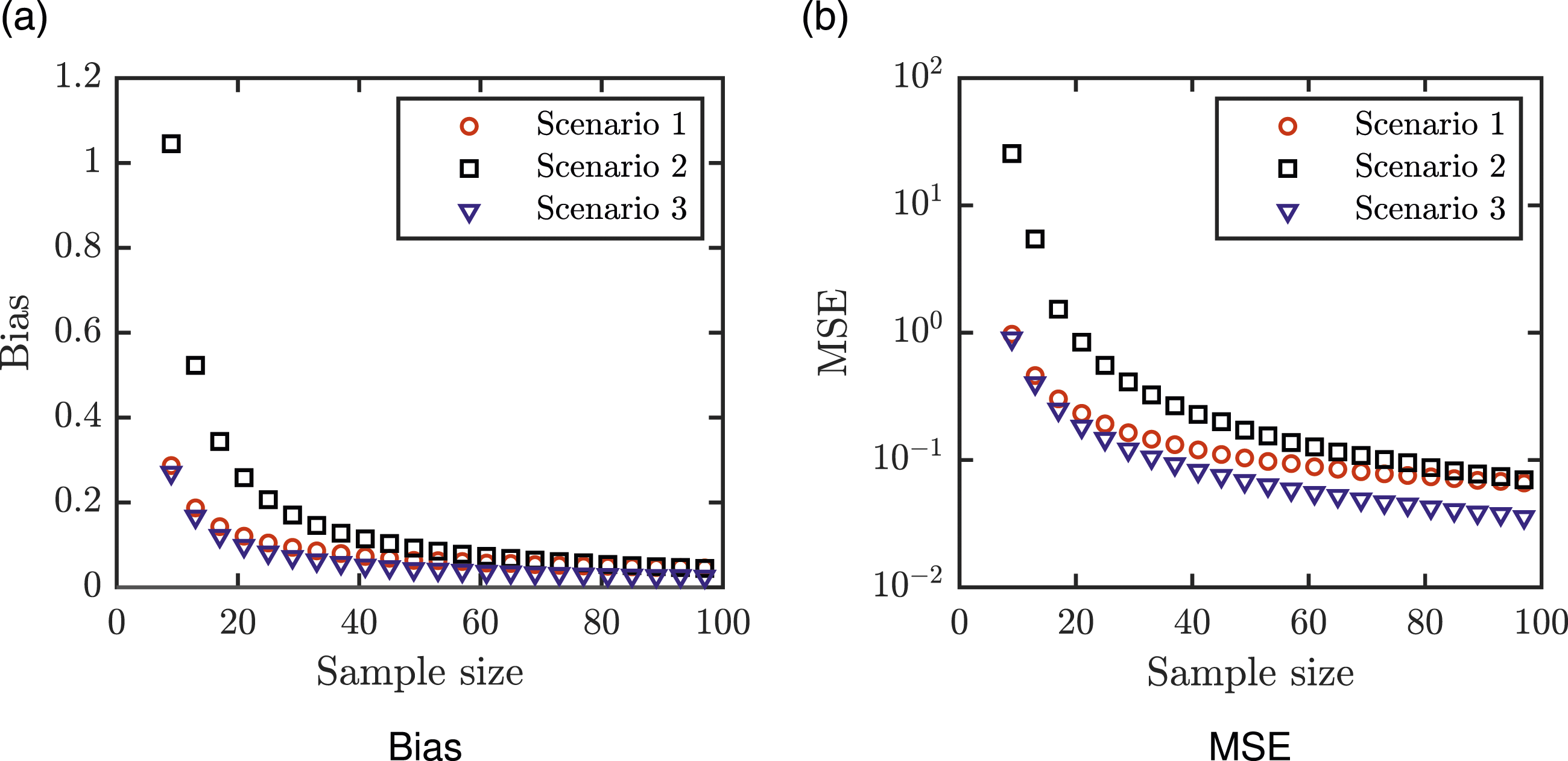

In this paper, we significantly simplify the method developed in Walter et al. ¹³ and propose unbiased estimators of σ⁻² from normally distributed data. The estimators can incorporate the knowledge of the interquartile range as well. Unfortunately, there are no closed formulas for those estimators, and so we searched for and obtained simple-to-use approximations that still show a little to no bias.

Methods

Scenario 1, {a, m, b; n}

Let us write

$\frac{1}{R_n^2}=\left(\frac{S_n^2}{R_n^2}\right)\left(\frac{1}{S_n^2}\right),$

(1)

where R _n = b − a is the sample range and S _n is the sample standard deviation. From Basu’s theorem, ¹⁶ we know that $S_n^2/R_n^2$ and $1/S_n^2$ are independent random variables since $S_n^2/R_n^2$ is free of σ² (and so is ancillary) and $S_n^2$ is a complete sufficient statistic for σ². Therefore, we have

$\mathbb{E}\left[\frac{1}{R_n^2}\right]=\mathbb{E}\left[\frac{S_n^2}{R_n^2}\right]\mathbb{·}\mathbb{E}\left[\frac{1}{S_n^2}\right]$

(2)

due to independence. Note that $\left(n-1\right)S_n^2/{\sigma }^2\sim {\chi }_{n-1}^2$ . Here, we have assumed the sample variance to have n − 1 as its denominator. If one were to use the sample variance with denominator n, then the only change that would result would be to use $n{S}_n^2/{\sigma }^2$ which has a chi-square distribution with n − 1 degrees of freedom in the formula derived subsequently. Thus,

$\mathbb{E}\left[\frac{1}{n-1}\frac{{\sigma }^2}{S_n^2}\right]=\frac{2^{\frac{n-1}{2}-1}\mathrm{\Gamma }\left(\frac{n-1}{2}-1\right)}{2^{\frac{n-1}{2}}\mathrm{\Gamma }\left(\frac{n-1}{2}\right)}=\frac{1}{2\left(\frac{n-1}{2}-1\right)}=\frac{1}{n-3},$

(3)

and so

$\mathbb{E}\left[\frac{1}{S_n^2}\right]=\left(\frac{n-1}{n-3}\right)\frac{1}{{\sigma }^2}.$

(4)

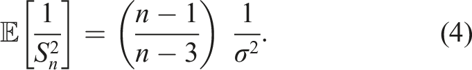
Let us denote $\mathbb{E}\left[S_n^2/R_n^2\right]$ by α _n . Then,

$\mathbb{E}\left[\frac{1}{R_n^2}\right]=\mathbb{E}\left[\frac{S_n^2}{R_n^2}\right]\mathbb{·}\mathbb{E}\left[\frac{1}{S_n^2}\right]={\alpha }_n·\left(\frac{n-1}{n-3}\right)\frac{1}{{\sigma }^2}.$

(5)

Thus, when we set

${\beta }_n=\frac{n-3}{\left(n-1\right){\alpha }_n},$

(6)

we get $\mathbb{E}\left[{\beta }_n/R_n^2\right]=1/{\sigma }^2$ , i.e., ${\beta }_n/R_n^2$ is an unbiased estimator of 1/σ².

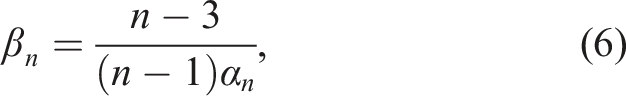
We note that there is no closed-form formula for β _n . However, as $S_n^2/R_n^2$ is free of μ and σ, we can obtain the value of α _n and consequently the value of β _n , by simulations over a large number of runs as described below in Section Numerical simulations. Furthermore, we can then approximate the simulated values of α _n and β _n by simple functions and thus obtain a simple-to-use estimator of 1/σ².

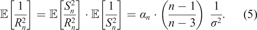
Scenario 2, {q₁, m, q₃; n}

As in scenario 1, let I _n = q₃ − q₁ be the interquartile range and let ${\gamma }_n=\mathbb{E}\left[S_n^2/I_n^2\right]$ . Let δ _n = (n − 3)/(n − 1)γ _n . Then, ${\delta }_n/I_n^2$ is an unbiased estimator of 1/σ². As above, we can use simulations to get values of γ _n and δ _n and obtain approximations for simple-to-use estimator.

Scenario 3 {a, q ₁ , m, q ₃ , b; n}

As in Shi et al., ¹⁴ we will get an unbiased estimator of σ⁻² if we take any linear combination of the two estimators presented above for Scenarios 1 and 2. We need to find the weights that yield the smallest variance.

For any w ∈ [0, 1], consider an estimator $w{\beta }_n/R_n^2+\left(1-w\right){\delta }_n/I_n^2$ . Let $R_n^{*}=R_n/{\sigma }^2$ and $I_n^{*}=I_n/{\sigma }^2$ be the range and interquartile range, respectively, for the standard normal distribution N(0, 1). Note that $\mathbb{E}\left[{\beta }_n/R_n^{*2}\right]=1$ and $\mathbb{E}\left[{\delta }_n/I_n^{*2}\right]=1$ . Thus,

$\text{Var}\left(w\frac{{\beta }_n}{R_n^2}+\left(1-w\right)\frac{{\delta }_n}{I_n^2}\right)=\frac{1}{{\sigma }^4}\left(w^2{V}_{1,n}+{\left(1-w\right)}^2{V}_{2,n}+2w\left(1-w\right)V_{3,n}\right),$

(7)

where

$\begin{array}{cc}{V}_{1,n}& =\text{Var}\left(\frac{{\beta }_n}{R_n^{*2}}\right)=\mathbb{E}\left[{\left(\frac{{\beta }_n}{R_n^{*2}}-1\right)}^2\right],\end{array}$

(8)

$\begin{array}{cc}{V}_{2,n}& =\text{Var}\left(\frac{{\delta }_n}{I_n^{*2}}\right)=\mathbb{E}\left[{\left(\frac{{\delta }_n}{I_n^{*2}}-1\right)}^2\right],\end{array}$

(9)

$\begin{array}{cc}{V}_{3,n}& =\text{Cov}\left(\frac{{\beta }_n}{R_n^{*2}},\frac{{\delta }_n}{I_n^{*2}}\right)=\mathbb{E}\left[\left(\frac{{\beta }_n}{R_n^{*2}}-1\right)\left(\frac{{\delta }_n}{I_n^{*2}}-1\right)\right]\end{array}.$

(10)

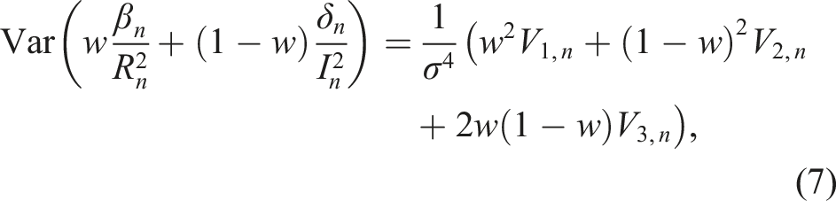
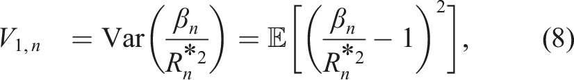
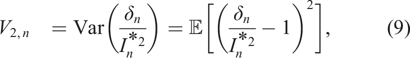
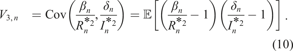
Minimizing (7) with respect to w ∈ (−∞, ∞), we get the equation

$2w{V}_{1,n}-2\left(1-w\right)V_{2,n}+2\left(1-2w\right)V_{3,n}=0.$

(11)

Thus, the optimal weight is given by

$w_{opt,n}=\frac{V_{2,n}-V_{3,n}}{V_{1,n}+V_{2,n}-2V_{3,n}}.$

(12)

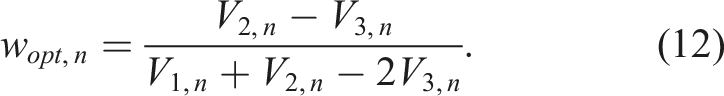
As before, while we could not obtain closed formulas for V_1,n, V_2,n and V_3,n, we can obtain their approximate values from the simulations. This in turn gives an approximate value of the optimal weight w_opt,n in (12). Moreover, the simulations yield w_opt,n ∈ (0, 1); if we had w_opt,n < 0 then we would have to use 0 as the optimal weight and, similarly, if w_opt,n > 1, we would have to use 1.

Numerical simulations

For every n ∈ {9, 13, 17, …, 97} = {4k + 1; k = 2, 3, …, 24}, we generated 10⁵ random samples of size n from N(0, 1). We restricted ourselves to n < 100 since, as seen in Figure 1, the indirect approximation has the highest bias and MSE for n < 50.

For each sample, we calculated the sample standard deviation S _n , sample range $R_n^{*}$ , and interquartile range $I_n^{*}$ . We then obtained values of α _n and γ _n as the average value of $S_n^2/R_n^{*2}$ and $S_n^2/I_n^{*2}$ , respectively, with which we obtained β _n = (n − 3)/(n − 1)α _n and δ _n = (n − 3)/(n − 1)γ _n . Similarly, we obtained values of V_1,n, V_2,n and V_3,n from formulas (8)–(10) and used those values to obtain a simulated value of w_opt,n by (12).

We calculated bias of the estimates as the average of ${\beta }_n/R_n^2-1/{\sigma }^2$ and ${\delta }_n/I_n^2-1/{\sigma }^2$ , respectively. The mean square error was calculated as the average of ${\left(\text{estimate}-{\sigma }^{-2}\right)}^2$ .

Finally, as in Wan et al., ⁸ we study the performance of the proposed estimators relative to the naïve methods using the state of the art estimators of σ from Shi et al. ¹⁴ for various distributions, specifically (a) normal distribution with μ = 50 and σ = 17, (b) log-normal distribution with μ = 4 and σ = 0.3, (c) beta distribution with α = 9 and β = 4, (d) exponential distribution with λ = 10, and (e) Weibull distribution with a = 2 and b = 35.

Results

Table 1 shows values of the constants α _n , β _n , γ _n , δ _n , w _n obtained by numerical simulations. We note that the coefficient β _n agrees with the Taylor series approximation method (with polynomial of order 4) developed in Walter et al. ¹³

Table 1.

The results of numerical simulations (rounded to four decimal places): n is the sample size; α _n is the simulated average of $S_n^2/R_n^2$ ; β _n = (n − 3)/(n − 1)α _n ; γ _n is the simulated average of $S_n^2/I_n^2$ ; δ _n = (n − 3)/(n − 1)γ _n ; w _n is the optimal weight of estimate E₁ From (20) in the case of Scenario 3. For every scenario, the Bias and MSE show bias and Mean Square Error of (independent) 10⁵ simulations of estimating σ⁻² by (18), (19), and (20), respectively.

	Scenario 1				Scenario 2				Scenario 3
n	α n	β n	Bias	MSE	γ n	δ n	Bias	MSE	w n	Bias	MSE
9	0.1095	6.8492	0.0022	0.5400	1.0580	0.7089	−0.0380	5.4088	0.9681	0.0044	0.5769
13	0.0890	9.3671	0.0014	0.3029	0.8238	1.0116	0.0230	2.3341	0.9395	0.0031	0.2964
17	0.0777	11.2607	−0.0004	0.2154	0.7412	1.1804	0.0223	0.8175	0.8561	0.0031	0.2002
21	0.0706	12.7412	0.0005	0.1738	0.6999	1.2859	0.0178	0.5075	0.7990	0.0041	0.1536
25	0.0655	14.0039	−0.0001	0.1486	0.6722	1.3636	0.0128	0.3603	0.7553	0.0031	0.1257
29	0.0617	15.0541	0.0002	0.1294	0.6512	1.4260	0.0053	0.2817	0.7283	0.0016	0.1056
33	0.0586	15.9885	0.0000	0.1172	0.6366	1.4727	0.0013	0.2316	0.7025	0.0004	0.0925
37	0.0561	16.8221	0.0001	0.1078	0.6271	1.5060	0.0016	0.1979	0.6812	0.0006	0.0828
41	0.0540	17.5840	−0.0016	0.0994	0.6206	1.5307	0.0025	0.1742	0.6640	−0.0001	0.0743
45	0.0523	18.2388	−0.0016	0.0924	0.6133	1.5565	0.0002	0.1553	0.6537	−0.0010	0.0681
49	0.0507	18.8846	−0.0028	0.0877	0.6082	1.5758	−0.0005	0.1364	0.6293	−0.0019	0.0624
53	0.0495	19.4271	−0.0005	0.0827	0.6027	1.5955	−0.0008	0.1250	0.6224	−0.0006	0.0579
57	0.0483	19.9654	0.0003	0.0801	0.5990	1.6098	0.0001	0.1128	0.6006	0.0002	0.0542
61	0.0472	20.4650	−0.0009	0.0761	0.5958	1.6226	0.0001	0.1055	0.5953	−0.0005	0.0510
65	0.0463	20.9308	0.0004	0.0732	0.5925	1.6350	0.0011	0.0975	0.5841	0.0007	0.0482
69	0.0454	21.3664	−0.0002	0.0703	0.5906	1.6435	0.0018	0.0925	0.5785	0.0006	0.0457
73	0.0446	21.7866	−0.0001	0.0679	0.5873	1.6554	0.0012	0.0866	0.5695	0.0004	0.0434
77	0.0439	22.1900	−0.0002	0.0662	0.5861	1.6613	0.0034	0.0827	0.5625	0.0014	0.0419
81	0.0433	22.5399	0.0006	0.0648	0.5833	1.6714	0.0016	0.0761	0.5457	0.0010	0.0398
85	0.0426	22.9036	0.0009	0.0630	0.5819	1.6777	0.0031	0.0725	0.5389	0.0019	0.0380
89	0.0421	23.2327	0.0006	0.0613	0.5803	1.6841	0.0028	0.0688	0.5320	0.0016	0.0366
93	0.0415	23.5493	0.0022	0.0602	0.5786	1.6906	0.0044	0.0662	0.5260	0.0032	0.0356
97	0.0411	23.8434	0.0022	0.0587	0.5777	1.6949	0.0043	0.0628	0.5180	0.0032	0.0339

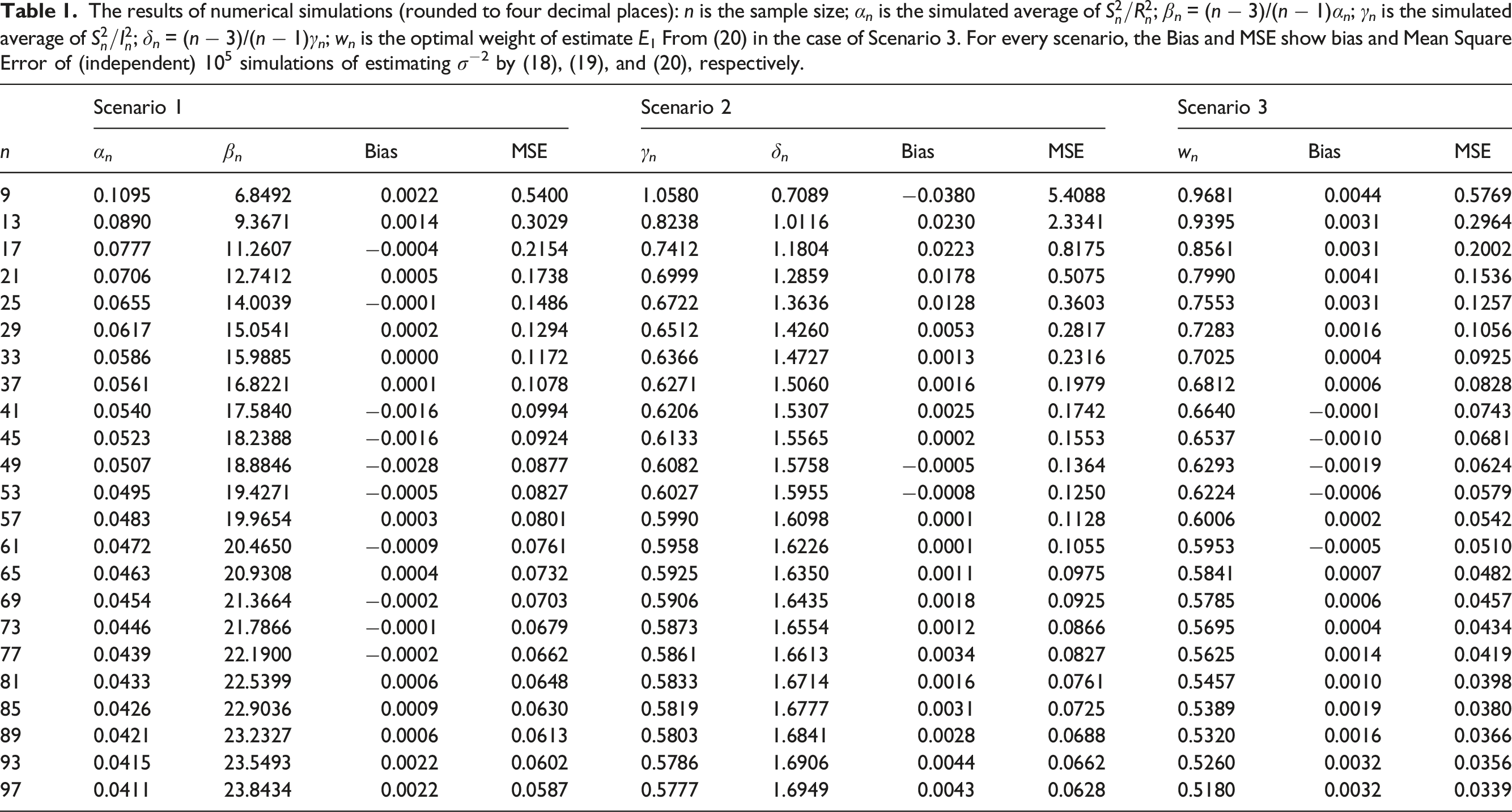
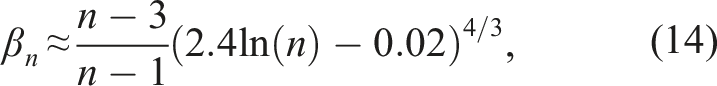
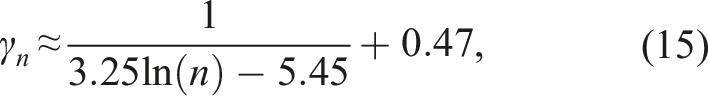
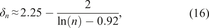
By trial and error, we discovered that ${\alpha }_n^{-0.75}$ , $w_{opt,n}^{-0.75}$ and 1/(δ _n − 2.25) are almost linear in ln n; see Figure 2. Applying linear regression then yields the following approximations.

$\begin{array}{l}{\alpha }_n\hspace{0.17em}\approx \hspace{0.17em}{\left(2.4\ln \left(n\right)-0.02\right)}^{-4/3},\end{array}$

(13)

$\begin{array}{c}{\beta }_n\hspace{0.17em}\approx \hspace{0.17em}\frac{n-3}{n-1}{\left(2.4\ln \left(n\right)-0.02\right)}^{4/3},\end{array}$

(14)

$\begin{array}{c}{\gamma }_n\hspace{0.17em}\approx \hspace{0.17em}\frac{1}{3.25\ln \left(n\right)-5.45}+0.47,\end{array}$

(15)

$\begin{array}{c}{\delta }_n\hspace{0.17em}\approx \hspace{0.17em}2.25-\frac{2}{\ln \left(n\right)-0.92},\end{array}$

(16)

$\begin{array}{c}{w}_{opt,n}\hspace{0.17em}\approx \hspace{0.17em}{\left(0.2727\ln \left(n\right)+0.3617\right)}^{-4/3}\end{array}.$

(17)

Figure 2.

Top row: approximating (a) ${\alpha }_n^{-0.75}$ , (b) $-{\left({\delta }_n-2.25\right)}^{-1}$ , and (c) $w_{opt,n}^{-0.75}$ , by functions linear in ln n. Bottom row: relative errors of the approximations (d) equations (13), (3) equations (16), and (f) equation (17).

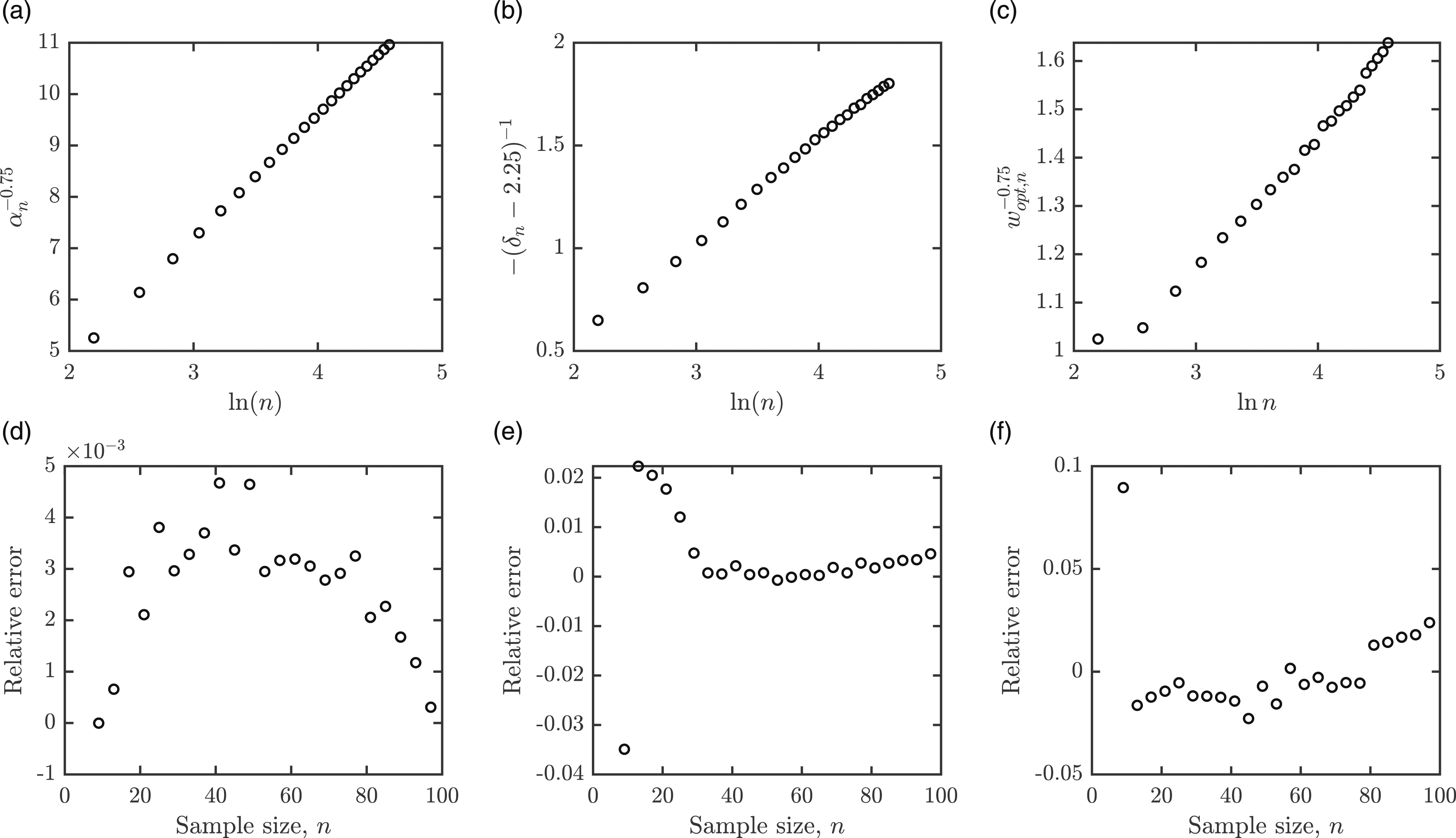
This yields the following unbiased estimators of 1/σ²:

$\begin{array}{c}{E}_1\hspace{0.17em}=\frac{\left(n-3\right){\left(2.4\ln \left(n\right)-0.02\right)}^{4/3}}{\left(n-1\right){\left(b-a\right)}^2},\end{array}$

(18)

$\begin{array}{l}{E}_2\hspace{0.17em}=\frac{2.25-\frac{2}{\ln \left(n\right)-0.92}}{{\left(q_3-q_1\right)}^2},\end{array}$

(19)

$\begin{array}{cc}{E}_3& =w_{opt,n}{E}_1+\left(1-w_{opt,n}\right)E_2.\end{array}$

(20)

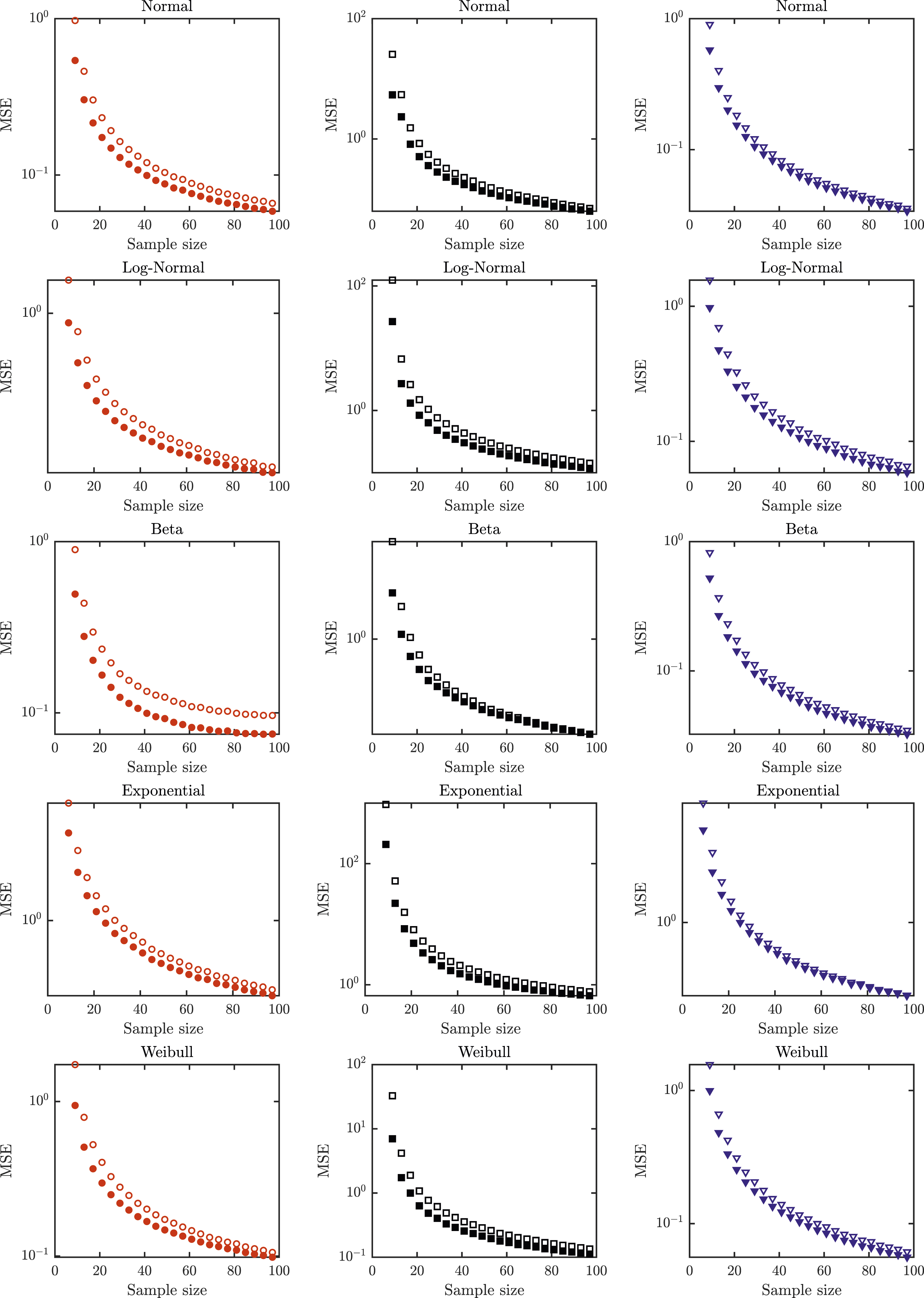
The estimator E _i is used in scenario i. The illustration that the estimators are unbiased and their mean square errors are shown in Figure 3.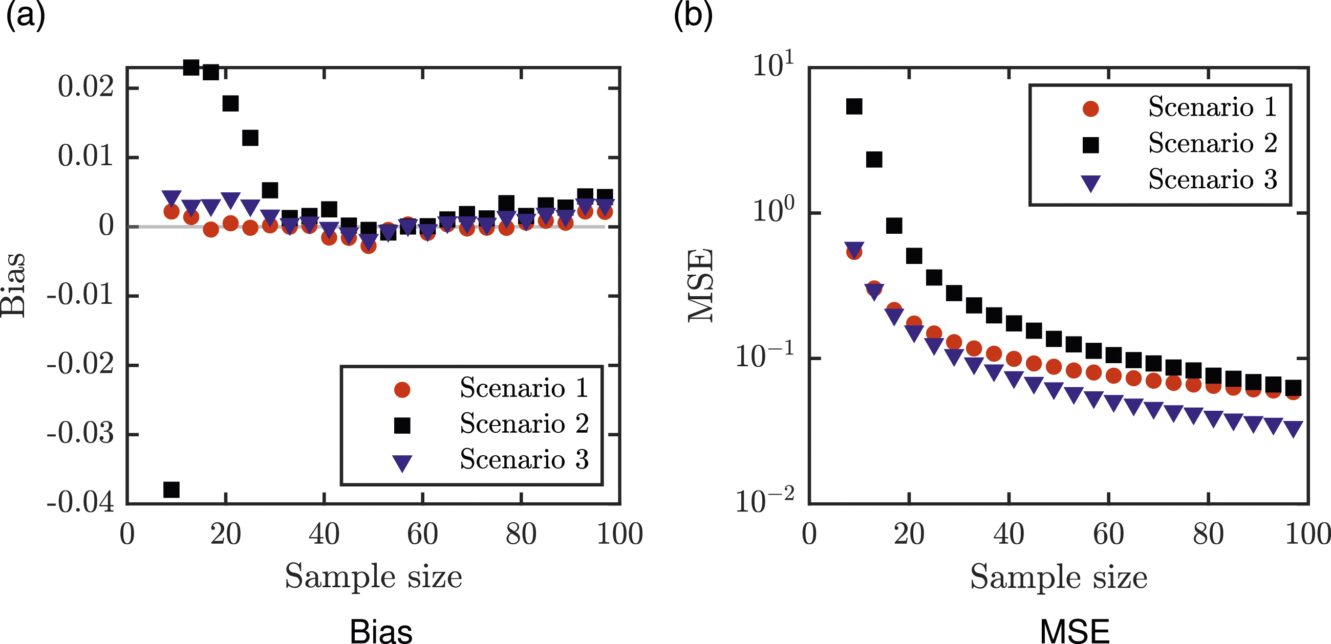

Figure 3.

Bias (a) and MSE (b) of estimating σ⁻² under various scenarios by estimators (18)–(20).

The performance of the proposed estimators for non-normal distributions is illustrated in Figures 4 and 5. We see that, in terms of MSE and generally also in terms of bias, the proposed estimators outperform the naïve method of estimating the standard deviation first and then raising it to power −2. The notable exception when bias is slightly smaller for the naïve methods are for n > 20 in Scenario 2 for beta distribution. The proposed methods also slightly underperform, in terms of bias, in Scenario 1 for n > 80 and log-normal or Weibull distributions.

Figure 4.

Bias of estimating σ⁻² by the newly proposed estimators (full markers) against the bias of the naïve method using the state of the art estimators from Shi et al. ¹⁴ (empty markers) for Normal distribution (first row), Log-normal distribution (second row), Beta distribution (third row), Exponential distribution (fourth row) and Weibull distribution (fifth row) and scenario 1 (left column), scenario 2 (middle column) and scenario 3 (right column).

Figure 5.

MSE (on a logarithmic scale) of estimating σ⁻² by the newly proposed estimators (full markers) against the MSE of the state of the art estimators from Shi et al. ¹⁴ (empty markers) for Normal distribution (first row), Log-normal distribution (second row), Beta distribution (third row), Exponential distribution (fourth row) and Weibull distribution (fifth row) and scenario 1 (left column), scenario 2 (middle column) and scenario 3 (right column).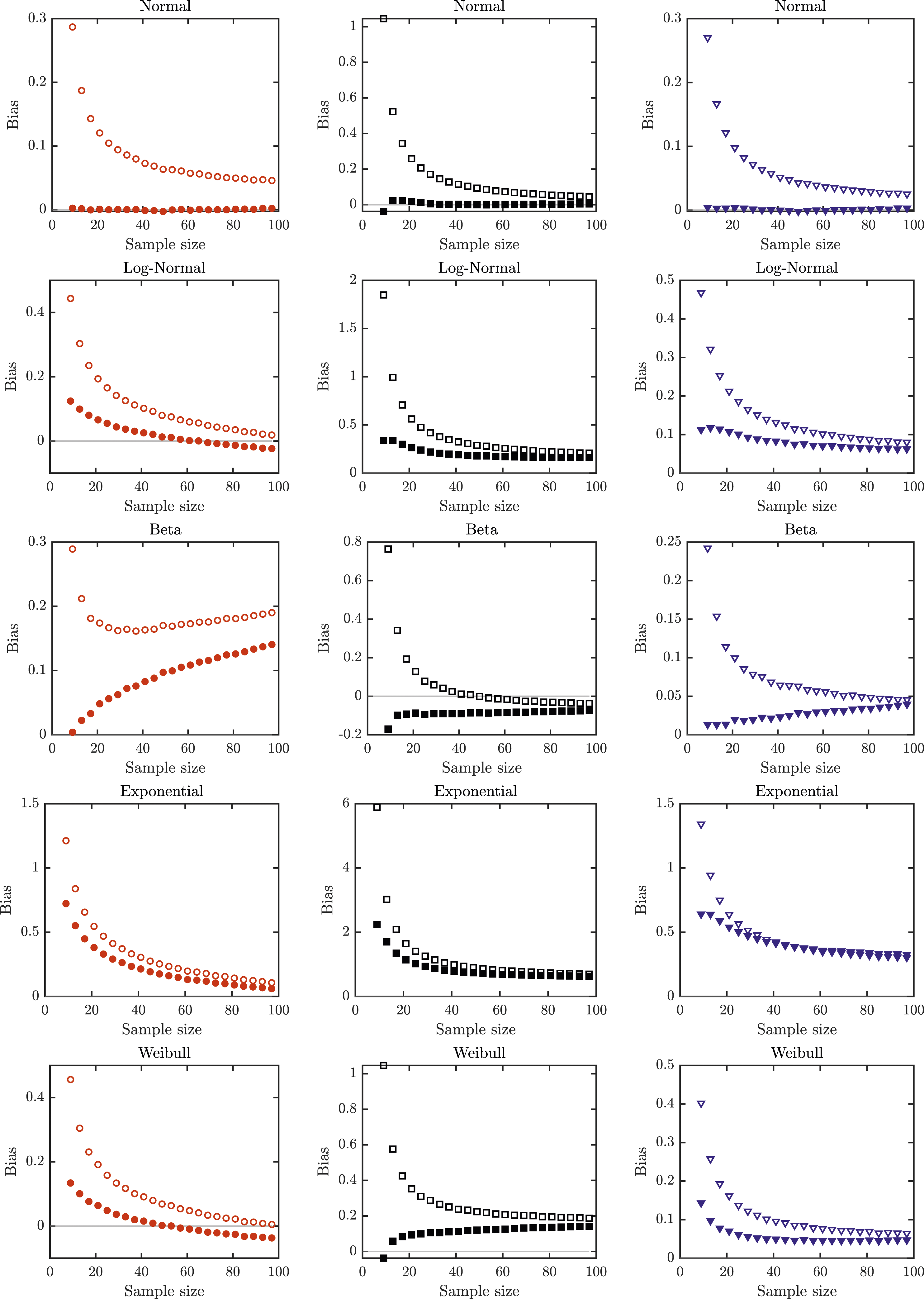

Real data example

To illustrate the use of the proposed method in proposed method in a single study which might then be incorporated into a meta-analysis, we took a dataset from Monaco et al. ³ which describes a randomised clinical trial on using tranexamic acid in open aortic aneurysm surgery. The dataset consists of two groups (experimental and control). Each group has n = 50 patients and for each patient, there are 7 continuous variables as described in Table 2. From the dataset, we estimated the inverse variance in each group separately, based on the individual data points, and taking the reciprocal of the standard estimate of the variance, i.e., s⁻² where s is the sample SD. We also estimated the appropriate quantiles and applied the proposed direct methods (18)-(20) as well as the indirect method of estimating σ first as in Shi et al. ¹⁴ and then raising it to the power −2.

Table 2.

Summary of the analysis performed on seven continuous variables from data from Monaco et al. ³ D = direct method as in (18)–(20). I = indirect method by estimating σ first as in Shi et al. ¹⁴

Variable	1 (104)	2 (103)	3 (106)	4 (104)	5 (105)	6 (106)	7 (101)
Experimental group (n = 50)
True s−2	3.71	5.894	1.19	4.864	5.071	1.087	4.546
D, Sc 1	2.921	4.638	0.5366	4.109	4.786	0.5047	2.968
I, Sc 1	3.11	4.937	0.5712	4.375	5.095	0.5373	3.16
D, Sc 2	5.849	8.069	4.393	9.885	6.583	2.471	15.82
I, Sc 2	6.072	8.377	4.561	10.26	6.834	2.565	16.42
D, Sc 3	4.029	5.936	1.996	6.295	5.466	1.249	7.83
I, Sc 3	3.984	6.03	1.056	5.944	5.716	0.8879	5.328
Control group (n = 50)
True s−2	4.198	4.999	2.528	2.512	5.438	2.281	7.449
D, Sc 1	3.925	3.664	1.569	1.596	5.022	1.348	7.598
I, Sc 1	4.178	3.901	1.671	1.699	5.346	1.435	8.089
D, Sc 2	5.849	4.881	3.743	3.228	3.763	3.985	15.82
I, Sc 2	6.072	5.067	3.886	3.351	3.907	4.137	16.42
D, Sc 3	4.653	4.125	2.392	2.213	4.546	2.346	10.71
I, Sc 3	4.829	4.324	2.264	2.184	4.674	2.075	10.49

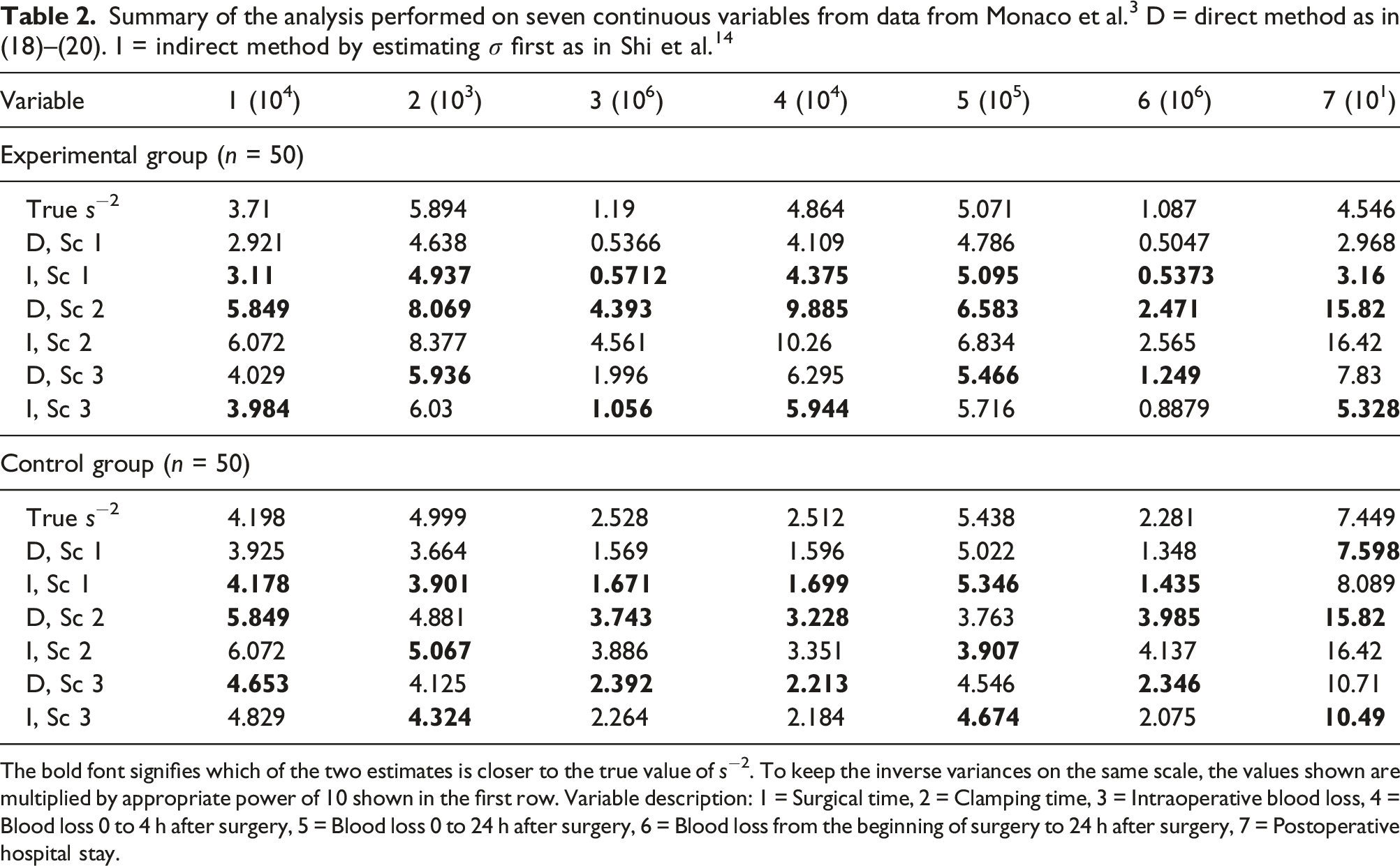
The bold font signifies which of the two estimates is closer to the true value of s⁻². To keep the inverse variances on the same scale, the values shown are multiplied by appropriate power of 10 shown in the first row. Variable description: 1 = Surgical time, 2 = Clamping time, 3 = Intraoperative blood loss, 4 = Blood loss 0 to 4 h after surgery, 5 = Blood loss 0 to 24 h after surgery, 6 = Blood loss from the beginning of surgery to 24 h after surgery, 7 = Postoperative hospital stay.

The summary is presented in Table 2. The data published in Monaco et al. ³ contained only the quartile values, so this corresponds to our Scenario 2. The proposed direct methods in Scenario 2 always outperform the indirect method in the experimental group and mostly (5 out 7) outperforms the indirect method in the control group. However, in this Scenario, both methods also yield the worst errors among the methods we considered. The estimated values are closer to s⁻² in Scenario 1 (when the indirect methods outperform the proposed method) and Scenario 3 (when the estimates are closest to the true value and the results are mixed). The goodness of the approximation is consistent with Figures 1 and 3 which show that, for n < 100, the MSEs in Scenario 3 are smaller than in Scenario 1 which are smaller than in Scenario 2.

Conclusions and discussion

The problem of estimating an unreported standard deviation from reported data summaries is an important problem in meta-analysis. Recently, unbiased methods with least MSE have been developed in Shi et al. ¹⁴ and Balakrishnan et al. ¹⁵ developed a unified approach that works for any reported summaries. However, even these optimal methods possess bias when used to estimate the inverse variance.

In this paper, we have developed a simple and efficient method for estimating the inverse variance directly. We have proved analytically that the proposed estimators are unbiased for normally distributed data. We obtained numerical values of the estimators through Monte Carlo simulations using which we have found simple-to-use approximations.

The proposed estimators were developed under the assumption that the data is normally distributed. Under this assumption, the proposed estimators outperform the naïve methods and even the best estimators from Shi et al. ¹⁴ and Balakrishnan et al. ¹⁵ both in terms of bias and MSE. However, the data distribution is typically not known and it thus important to estimate the robustness of the proposed method. We saw that the proposed estimators also improve MSE, and almost always (except for the exponential distribution and large n) possess lower bias, over the naïve methods even for data that are not normally distributed.

Therefore, when the inverse variance is the true quantity of interest, for pooling purposes, for example, one should estimate it directly using the estimators presented in this paper.