Statistical assessment of the prognostic and the predictive value of biomarkers-A biomarker assessment framework with applications to traumatic brain injury biomarker studies

Abstract

Studies that investigate the performance of prognostic and predictive biomarkers are commonplace in medicine. Evaluating the performance of biomarkers is challenging in traumatic brain injury (TBI) and other conditions when both the time factor (i.e. time from injury to biomarker measurement) and different levels or doses of treatments are in play. Such factors need to be accounted for when assessing the biomarker’s performance in relation to a clinical outcome. The Hyperbaric Oxygen in Brain Injury Treatment (HOBIT) trial, a phase II randomized control clinical trial seeks to determine the dose of hyperbaric oxygen therapy (HBOT) for treating severe TBI that has the highest likelihood of demonstrating efficacy in a phase III trial. Hyperbaric Oxygen in Brain Injury Treatment will study up to 200 participants with severe TBI. This paper discusses the statistical approaches to assess the prognostic and predictive performance of the biomarkers studied in this trial, where prognosis refers to the association between a biomarker and the clinical outcome while the predictiveness refers to the ability of the biomarker to identify patient subgroups that benefit from therapy. Analyses based on initial biomarker levels accounting for different levels of HBOT and other baseline clinical characteristics, and analyses of longitudinal changes in biomarker levels are discussed from a statistical point of view. Methods for combining biomarkers that are of complementary nature are also considered and the relevant algorithms are illustrated in detail along with an extensive simulation study that assesses the performance of the statistical methods. Even though the discussed approaches are motivated by the HOBIT trial, their applications are broader. They can be applied in studies assessing the predictiveness and prognostic ability of biomarkers in relation to a well-defined therapeutic intervention and clinical outcome.

Introduction

Currently, there are no therapeutic agents that have been shown to improve outcomes for patients with severe traumatic brain injury (TBI). Critical barriers to progress in developing treatments for severe TBI are the lack of predictive biomarkers for identifying patients likely to benefit from a promising intervention, as well as the lack of prognotic biomarkers for early and accurate prognostication of clinical outcomes. Clinical examination and brain CT imaging remain the fundamental tools for the initial evaluation of patients with severe TBI and for subject selection in clinical trials. Blood-based biomarkers might serve as adjunctive tools to clinical examination and CT imaging. They could make clinical trials more efficient by enabling the enrollment of subjects that are most likely to derive benefit. Three promising biomarkers that may be useful as both prognostic and predictive biomarkers in clinical trials involving patients with severe TBI are Glial fibrillary acidic protein (GFAP), neurofilament light chain (NfL) and high sensitivity c-reactive protein (hsCRP). Glial fibrillary acidic protein and NfL are structural proteins found in astrocytes and neurons, respectively, and they are released after a TBI in amounts that are proportional to anatomic injury severity; their levels are correlated with TBI lesion volume as measured by head CT and they can quantify the extent of neuronal and glial loss following TBI.^1–4 Levels of hsCRP, a nonspecific marker of inflammation, may complement the anatomic biomarkers since dysfunction in TBI is also highly mediated by neuroinflammation. ⁵

Current gaps in knowledge limit the use of these biomarkers in TBI clinical trials. First, in human randomized control trials it is currently unknown whether a promising neuroprotective agent will have a treatment effect on these biomarkers, or whether the achievement of substantial treatment effects on these biomarkers reliably predicts clinical outcome. A poor clinical outcome is associated with a Glasgow Outcome Scale Extended (GOSE) score that is ≤4 while a favorable outcome refers to a score $>r\mathrm{b}\mathrm{i}\mathrm{n}4$ (see ⁶ ). It is unknown whether baseline levels of these biomarkers are useful for subject selection in a clinical trial of a neuroprotective agent.

To address these questions and knowledge gaps, we are conducting a biomarker study that includes longitudinal measurements of three biomarkers (GFAP, NfL, and hsCRP) in the Hyperbaric Oxygen in Brain Injury Treatment (HOBIT) trial. The HOBIT trial will enroll up to 200 severe TBI subjects. It is a phase II randomized control clinical trial that seeks to determine the dose of hyperbaric oxygen therapy (HBOT) that has the highest likelihood of demonstrating efficacy in a subsequent phase III trial. The key biological pathways through which HBOT affects clinical outcome are: (1) a decrease in neural cell lose (which can be measured by GFAP and NfL); and (2) a decrease in systemic inflammation (which can be measured by hsCRP). The main mechanism is improvement in oxidative metabolism which improves the energy depletion of severe TBI. A decrease in inflammatory markers in the brain has also been discussed in basic animal research studies (see Do and Woo, 2018 among others).

The goal of this manuscript is to illustrate the appropriate statistical methodologies and relevant modeling approaches for addressing these questions. Our aim is to provide statistical guidance for researchers that are interested in assessing the prognostic and predictive ability of biomarkers both at baseline and during subsequent follow-up measurements. We describe appropriate statistical strategies that accommodate biomarkers that are prognostic or predictive. In this paper, we discuss the differences between a prognostic and a predictive biomarker as well as the implications for the Receiver Operating Characteristic (ROC) analysis. We further discuss a statistical framework for assessing the performance of biomarkers at baseline. This involves a ROC analysis at baseline that aids in assessing the prognostic value of markers as well as the estimation of a cutoff for each marker that might be indicative of a subgroup that derives the most benefit from an experimental therapy. We illustrate the framework for adjusting for covariates that will make the cutoff estimation personalized as opposed to a ‘one size fits all’ notion. We illustrate how these covariates can be accommodated through Cox regression models even though we do not operate under a survival analysis framework. Such a proposed framework allows for natural assumptions such as a stochastic ordering between the biomarker distribution for the ‘favorable outcome group’ (D = 0) and the ‘unfavorable outcome group’ (D = 1) as defined by the GOSE scale. We illustrate how one can combine biomarkers that may carry complementary information, and we provide an algorithm for the maximization of the area under the ROC curve (AUC) along with the appropriate software for its application. We further discuss the estimation of probabilities of an unfavorable outcome given the biomarker values and the baseline characteristics based on a logistic regression model, its link to a ROC analysis, along with an alternative Cox-based approach.

For the assessment of biomarkers that are time-dependent, we illustrate the use of both a generalized estimating equations (GEE) framework as well as a mixed modeling framework, and we highlight the advantages and disadvantages of both. We also present simulations that evaluate the discussed approaches, illustrate their implementation, and provide insight into their utility. We end with a discussion about conclusions and limitations.

Prognostic and predictive biomarkers

Distinguishing prognostic biomarkers and predictive biomarkers may be a challenging task. Biomarkers measured at baseline that can identify the likelihood of a clinical outcome, disease progression or an event of interest are known as prognostic biomarkers. Intrinsic clinical characteristics often can also be considered as prognostic (bio-)markers since they may be indicative of the final outcome of interest. Prognostic biomarkers may be used as part of the eligibility criteria for a clinical trial that enrolls patients who are at risk for an unfavorable outcome. For example, if a prognostic biomarker can determine at baseline those who will end up experiencing a favorable outcome from others that may not, then the latter group may be of interest for recruitment to an experimental therapy/study. Identifying prognostic biomarkers usually involves observational data.

On the other hand, predictive biomarkers are biomarkers that are used to identify patients that are more likely to exhibit a favorable outcome when treated with a specific therapy. For example, the control group may be receiving a standard therapy and comparisons are to be made against the experimental group that receives a new therapy. As discussed by the FDA, ⁷ prognostic biomarkers and predictive biomarkers cannot generally be distinguished when only patients who have received a particular therapy are studied. Generally, to identify a predictive biomarker, one needs to have a comparison of a ‘control group’ versus a ‘treatment group’. In addition, a biomarker can be prognostic, predictive, or both. A more detailed discussion with some graphical examples is provided therein.

Baseline analysis for the TBI biomarkers

Receiver operating characteristic curves at baseline to assess the prognostic value for each biomarker

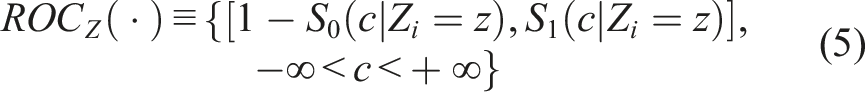
In this context, we will mainly focus on our control group, for which the same standard of care is administered. To assess whether the baseline biomarkers are prognostic, we need to investigate whether the baseline biomarker scores are different for those individuals that ended up having a favorable outcome (D = 0) versus those that ended up with an unfavorable outcome (D = 1). The ROC is the most popular statistical tool to evaluate the discriminatory ability of biomarkers between two groups (here these are D = 0 vs D = 1). The biomarker score of interest, taken to be a continuous variable denoted with Y, is then evaluated typically in terms of specificity and sensitivity. These probabilities can be written in terms of false positive rates (FPR) and true positive rates (TPR) as spec(c) = P(Y < c|D = 0) = 1 − FPR and sens(c) = P(Y > c|D = 1) = TPR(c) for an arbitrary cutoff c. Note that the specificity equals to F_Y|D = 0(c) = F₀(c) while the sensitivity equal⋅s to S_Y|D = 1(c) = 1 − F_Y|D = 1(c) (for which we use the notation S₁(c) = 1 − F₁(c) for simplicity) where F(⋅) denotes a cumulative distribution function and S(⋅) = 1 − F(⋅) the corresponding survival function. The ROC is the tradeoff of all pairs of sensitivities and specificities as we scan the cutoff c on the real line (see Pepe ⁸ and Zhou et al. ⁹ for more details). Namely

$\begin{array}{c}\mathit{R}\mathit{O}\mathit{C}\equiv \left\{\left(\mathit{F}\mathit{P}\mathit{R}\left(c\right),\mathit{T}\mathit{P}\mathit{R}\left(c\right)\right),-\infty <c<+\infty \right\}\end{array}$

(1)

The ROC has a more convenient representation through the underlying cumulative distribution functions of the two groups, or equivalently, their survival functions. This is of the form

$\begin{array}{c}\mathit{R}\mathit{O}\mathit{C}\left(t\right)=S_1\left(S_0^{-1}\left(t\right)\right),0<t<1.\end{array}$

(2)

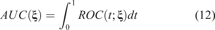
The AUC provides an overall measure of the degree of separation between F₁ and F₀. In particular, the AUC is the average sensitivity for all values of specificity (or the average specificity for all values of sensitivity). It is defined by

$\begin{array}{c}\mathit{A}\mathit{U}\mathit{C}={\int }_0^1\mathit{R}\mathit{O}\mathit{C}\left(t\right)dt.\end{array}$

(3)

In our trial, the biomarkers at baseline depend on some baseline characteristics of the participants, denoted here by Z. A modeling approach that is appropriate for accounting for the baseline characteristics in our framework is the well known Cox ¹⁰ -model. For a detailed and practical review of such a modeling approach we refer the reader to Klein and Moeschberger. ¹¹ Note that, even though Cox-modeling is very common for modeling survival data and is typically used in survival studies, its utility can be broader. In our study we do not focus on a ‘time to an event’ variable. In particular, at this point, we are only interested in the performance of the biomarker at baseline, and thus we will not even consider a repeated measures framework (which is discussed in the second part of this paper). Yet, a Cox model can be used to obtain an estimate of the cumulative distribution of the biomarker scores for those who had a favorable outcome (D = 0) and for those who did not, given a baseline profile (Z) of the participants. A Cox model can, by construction, provide an estimator for F₀(y|Z), or equivalently 1 − S₀(y|Z). The models for the favorable outcome (D = 0) and the unfavorable outcome (D = 1) are of the form

$\begin{array}{cc}{S}_0\left(y|Z,D=0\right)& =S_{\mathit{b}\mathit{a}\mathit{s}{\mathit{e}}_0}{\left(y\right)}^{\mathit{exp}\left({\mathit{\beta }}_{\mathbf{1}}Z\right)},\\ S_1\left(y|Z,D=1\right)& =S_{\mathit{b}\mathit{a}\mathit{s}{\mathit{e}}_1}{\left(y\right)}^{\mathit{exp}\left({\mathbf{\gamma }}_{\mathbf{1}}Z\right)},\end{array}$

(4)

and alternatively their smoothed hazard constrained natural spline (HCNS) versions (see Bantis, et al. ¹² ) may be used (software available at https://www.leobantis.net). To assess whether a biomarker is prognostic, it is enough to show that it can discriminate between the two groups (favorable outcome (D = 0) vs unfavorable outcome (D = 1)). To create the ROC curve that reflects such a discriminatory ability (or prognostic ability in this setting) we can consider

$\begin{array}{c}\mathit{R}\mathit{O}{\mathit{C}}_Z(·)\equiv \{\left[1-S_0\left(c|Z_i=z\right),S_1\left(c|Z_i=z\right)\right],\\ -\infty <c<+\infty \}\end{array}$

(5)

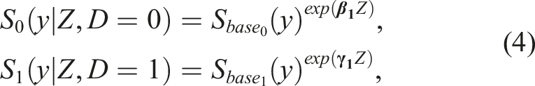
The area under it can be employed to assess the overall prognostic ability of the biomarker to detect those participants with a favorable outcome from those with an unfavorable outcome. The ROC defined in (5), is formulated for any desired baseline profile of characteristics. This in turn allows us to explore the prognostic performance of the biomarker given a specific baseline profile that might be of clinical interest. It can be the case that the prognostic ability of a biomarker is higher for some specific baseline profiles and lower or even poor for others.

In the case where the baseline information does not affect the biomarker values, we can directly construct the ROC based on expression (2) and assess the discriminatory ability through the AUC presented in (3). To determine a cutoff beyond which an individual of the control group is more likely to exhibit an unfavorable outcome, we utilize the Youden index (see Youden ¹³ ). This can be applied not only to the standard of care arm in a clinical trial, but to other arms as well. We hope to observe that the Youden index cutoff will be affected by the dose. This will allow us to calculate the probabilities that an individual of a given arm has a favorable outcome based on the arm’s cutoff. The Youden-based cutoff is given by

$\begin{array}{c}{c}^{*}=\mathit{a}\mathit{r}\mathit{g}\mathit{m}\mathit{a}{\mathit{x}}_c\left\{\mathit{S}\mathit{e}\mathit{n}\mathit{s}\left(c\right)+\mathit{S}\mathit{p}\mathit{e}\mathit{c}\left(c\right)-1\right\},\\ -\infty <c<+\infty \end{array}$

(6)

For parametric and non-parametric methods regarding the estimation and the corresponding confidence intervals of the maximized Youden index and the Youden-based cutoff we refer to Bantis et al. ¹⁴ In the case where some variables contained in the baseline information (Z) are statistically significant after fitting the Cox-models presented above, our proposed Youden-based cutoffs are given by

$c^{*}=\mathit{a}\mathit{r}\mathit{g}\mathit{m}\mathit{a}{\mathit{x}}_c\left\{S_0\left(c|Z\right)-S_1\left(c|Z\right)\right\},-\infty <c<+\infty$

(7)

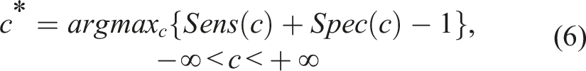
Note that this form of the Youden index i.e. max _c {S₀(c|Z) − S₁(c|Z)}, is personalized in the sense that different cutoff values are provided for different baseline profiles, Z. An interesting graphical aspect is that the cutoff presented in (7) is the maximum vertical distance of the ROC defined in (5) from the uninformative main diagonal of the unit square (see Bantis, et al. ¹⁵ and Fluss, et al. ¹⁶ ).

In cases where the baseline profile is of no statistical significance, the optimized cutoff degenerates to a unique cutoff (in the sense that it will not be different for different baseline profiles). The biomarker performance on such a cutoff can be summarized by estimating the sensitivity (TPR) and the specificity (1 − FPR) at such a cutoff, c^*. If the TPR and the FPR values at c^*, within a given arm, approach the value of 1, this implies that the marker can almost perfectly separate those who will exhibit an unfavorable outcome from those who will not.

Note that the cutoff c^* given in (6) is determined by the intersection of the underlying densities of those who had a favorable outcome and those who did not. Similarly, the cutoff c^* given in (7) is determined by the intersection of the underlying densities of those who had a favorable outcome and those who did not, given their baseline profile. Equivalently, this implies that the optimal cutoff is located at the point where the density ratio $f_1\left(c|Z_i\right)/f_0\left(c|Z_i\right)$ = 1. Generally, this would involve a study of the monotonicity of this density ratio to ensure uniqueness of the cutoff, given the baseline covariate profile. An alternative modeling approach would be to include the outcome (D) as a covariate in a single Cox-model

$\begin{array}{c}S\left(y|Z\right)=S_{\mathit{b}\mathit{a}\mathit{s}\mathit{e}}{\left(y\right)}^{\mathit{exp}\left({\mathit{\beta }}_{\mathbf{1}}Z+{\beta }_{2}D\right)}.\end{array}$

(8)

Such a formulation implies that given a favorable outcome we get $P\left(Y>y|Z,D=0\right)=S_{\mathit{b}\mathit{a}\mathit{s}\mathit{e}}{\left(y\right)}^{\exp \left({\mathit{\beta }}_{\mathbf{1}}Z\right)}$ while for an unfavorable outcome this is expressed by $P\left(Y>y|Z,D=1\right)=S_{\mathit{b}\mathit{a}\mathit{s}\mathit{e}}{\left(y\right)}^{\exp \left({\mathit{\beta }}_{\mathbf{1}}Z+{\beta }_2\right)}$ . This in turn implies that

$\begin{array}{cc}\frac{S\left(y|Z,D=1\right)}{S\left(y|Z,D=0\right)}& =\frac{P\left(Y>y|Z,D=1\right)}{P\left(Y>y|Z,D=0\right)}\\ & =\frac{S_{\mathit{b}\mathit{a}\mathit{s}\mathit{e}}{\left(y\right)}^{\mathit{exp}\left({\mathit{\beta }}_{\mathbf{1}}Z+{\beta }_2\right)}}{S_{base}{\left(y\right)}^{\mathit{exp}\left({\mathit{\beta }}_{\mathbf{1}}Z\right)}}\\ =S_{\mathit{b}\mathit{a}\mathit{s}\mathit{e}}{\left(y\right)}^{\left[\mathit{exp}\left({\mathit{\beta }}_{\mathbf{1}}Z\right)\right]\left[\mathit{exp}\left({\beta }_2\right)-1\right]}\end{array}$

(9)

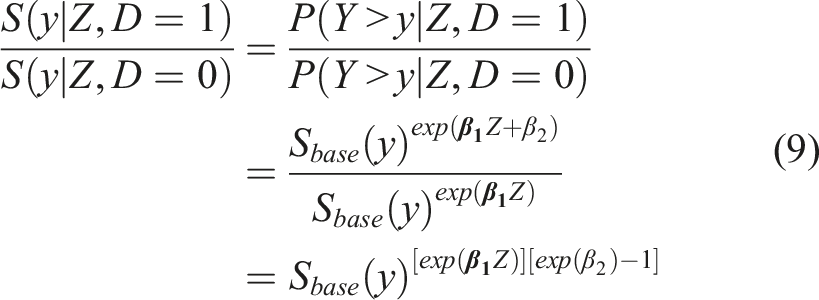
Note that for a given Z, the ratio of the cumulative distribution function of the biomarker scores for the group with the unfavorable outcome (D = 1) over those with a favorable outcome D = 0 is also $>0$ . Note that under this formulation

$\begin{array}{c}{S}_{\mathit{b}\mathit{a}\mathit{s}\mathit{e}}{\left(y\right)}^{\left[\mathit{exp}\left({\mathit{\beta }}_{\mathbf{1}}Z\right)\right]\left[\mathit{exp}\left({\beta }_2\right)-1\right]}<1\Rightarrow \frac{1-F\left(y|Z,D=1\right)}{1-F\left(y|Z,D=0\right)}<1\\ \Rightarrow F\left(y|Z,D=1\right)>F\left(y|Z,D=0\right)\end{array}$

(10)

and the result is analogous if we consider the case where the left-hand side is $>1$ . That is, for any y, the distributions of the two groups are stochastically ordered. When implementing model (8) we have the luxury of increased power and a natural assumption of stochastically ordered distributions at the cost of some flexibility. When implementing two separate models as in (4) we lose these advantages, but we gain flexibility in the following sense: we allow the baseline characteristics contained in Z to have a different impact on the ‘favorable outcome’ group compared to the impact they have on the ‘unfavorable outcome’ group.

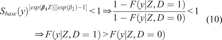
Whether formulation (8) or (4) is preferrable depends on the data set at hand, and in particular, on whether the underlying assumptions are plausible. It could be the case that a baseline characteristic affects the biomarker scores of the ‘favorable outcome’, yet it has no (or simply a different) impact for the ‘unfavorable outcome’ group (or vice versa). In that case, formulation (8) might be more preferable than that of (4). Such claims can also be explored by fitting the models and assessing whether the impact of Z is different between the two groups. Alternatively, one could employ a unified Cox model that further incorporates the arms as an additional covariate. This would increase power, but would come at a cost of flexibility. Note that for each new covariate one adds to the Cox model, we need to be willing to assume a more strict condition related to the type of stochastic ordering. Note that for each new covariate one adds to the Cox model, we need to be willing to assume a more strict condition related to the type of stochastic ordering. This is reflected by the inequality presented in (10) that may involve more than a single covariate. This assumptions needs to be assessed in a case by case manner with appropriate testing, and input from subject matter experts should be taken into account.

Note that even though the discussion so far has focused on the prognostic value of the baseline measurements, it can also be assessed when biomarker measurements are taken repeatedly over time. A framework in how to deal with such longitudinal settings is discussed later on.

Combining biomarkers at baseline to increase the individual prognostic value of each marker

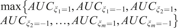
Multiple (k) biomarkers are to be collected at baseline (their measurements are denoted with Y⁽¹⁾, Y⁽²⁾, …, Y^(k)). Since they may carry complementary information, a combination of biomarkers may be more preferable in terms of separating those with a favorable outcome from those with an unfavorable outcome. If we focus on the family of linear combinations that is of the form

$\begin{array}{c}Y={\xi }_1{Y}^{\left(1\right)}+{\xi }_2{Y}^{\left(2\right)}+\dots +{\xi }_k{Y}^{\left(k\right)}\end{array}$

(11)

then interest lies in determining those coefficients ξ₁, ξ₂, …, ξ _k that are optimal in some sense. One natural criterion is the maximization of the AUC. The AUC of such a linear combination can be written as a function of the ξ vector that contains all ξ _i ’s and is simply the following integral

$\mathit{A}\mathit{U}\mathit{C}\left(\mathbf{\xi }\right)={\int }_0^1\mathit{R}\mathit{O}\mathit{C}\left(t;\mathbf{\xi }\right)dt$

(12)

where ROC(t; ξ) is the ROC that corresponds to the composite score Y. The goal is to find the optimal linear coefficients ξ^* that maximize the AUC(ξ), i.e.

${\mathbf{\xi }}^{*}=\arg \underset{\mathbf{\xi }}{\max }\mathrm{A}\mathrm{U}\mathrm{C}\left(\mathbf{\xi }\right)$

(13)

It is known in the literature that in such formulations, a smooth ROC will alleviate numerical problems regarding the optimization of the AUC and in such scenarios one can employ kernel based approaches. A kernel based approach that is discussed in Yan et al. ¹⁷ is based on the usual kernel density estimator (for a biomarker Y) given by

$\begin{array}{c}{\widehat{f}}_j\left(z\right)=\frac{1}{n_j{h}_j}{\displaystyle \sum }_{i=1}^{n_j}K\left(\frac{z-Y_{ji}}{h_j}\right),j=\mathrm{0,1}\\ \mathrm{a}\mathrm{n}\mathrm{d}\hspace{0.17em}i=\mathrm{1,2},\dots ,n_j\end{array}$

(14)

where $K\left(t\right)=1/\sqrt{2\pi }{e}^{-t^2/2}$ and h _j are the two bandwidths, one for each group. For a nice review of kernel density estimation we refer to Wand. ¹⁸ For the bandwidth one could use a simple plug in bandwidth like $h_0=0.9\min \left(sd\left(Y_0\right),\mathrm{I}\mathrm{Q}\mathrm{R}\left(Y_0\right)\right)n_0^{-0.2}$ as given by Silverman. ¹⁹ The expression for h₁ that refers to the ‘unfavorable outcome group’ (D = 0) is analogous. After obtaining the kernel density estimates we can construct the kernel-based ROC using $\mathrm{R}\widehat{\mathrm{O}}\mathrm{C}={\widehat{S}}_1\left({\widehat{S}}_0^{-1}\left(t\right)\right)$ , 0 < t < 1, that involves the kernel-based survival functions ${\widehat{S}}_0$ and ${\widehat{S}}_1$ derived with appropriate integration from the densities ${\widehat{f}}_0\left(z\right)$ and ${\widehat{f}}_1\left(z\right)$ mentioned above. Given the densities we can construct the corresponding ROC, which in turn allows us to straightfrowardly obtain the AUC. It is easy to see that the resulting AUC is a function of the coefficients ξ. For the maximization of the AUC one can employ standard optimization routines. We have observed through our simulations that the Nelder-Mead simplex method works well and it is readily available in both MATLAB and R through the function ‘fminsearch’.

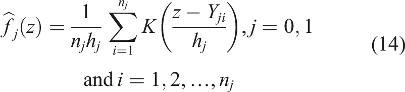
An advantage of a kernel-based approach is the resulting smoothness of the ROC which alleviates potential numerical problems. This is highlighted by Yin and Tian ²⁰ among others. Nonetheless, uniqueness of vector ξ cannot be ensured unless strict assumptions that relate to the concavity of the ROC are in play. We refer the interested reader to Yan et al. ¹⁷ for more comments on that aspect. Such an assumption is most likely not met in practice, and this comes at the risk of a non-unique solution, i.e. a non-unique ξ that maximizes the AUC. Yan et al. ¹⁷ employ the following algorithm that seems to work well in practice in minimizing the cases in which one is trapped to local maxima, especially when the underlying covariance matrices are not proportional and/or normality of the markers cannot be assumed. However, even though their approach alleviates that problem, there is still no guarantee that the obtained ξ corresponds to a global maximum. Their algorithm is the following:

Combination Algorithm:

• Step 1: Set the first biomarker as an anchor and set its coefficient, ξ₁ equal to 1.

• Step 2: Scan the remaining coefficients in the interval [ − 1, 1], and solve the optimization problem stated in (13).

• Step 3: Repeat Steps 1 and 2 by forcing ξ₁ equal to −1. Denote the maximized AUCs that correspond to ξ₁ = 1 and ξ₁ = −1 to $\mathrm{A}\mathrm{U}{\mathrm{C}}_{{\xi }_1=1}$ and $\mathrm{A}\mathrm{U}{\mathrm{C}}_{{\xi }_1=-1}$ respectively.

• Step 4: Repeat Steps 1 to 3 for each biomarker. Namely, proceed consecutively with the next biomarker as an anchor. Thus, the optimal AUC is equal to:

$\begin{array}{c}\max \{\mathit{A}\mathit{U}{\mathit{C}}_{{\xi }_1=1},\mathit{A}\mathit{U}{\mathit{C}}_{{\xi }_1=-1},\mathit{A}\mathit{U}{\mathit{C}}_{{\xi }_2=1},\\ \mathit{A}\mathit{U}{\mathit{C}}_{{\xi }_2=-1},\dots ,\mathit{A}\mathit{U}{\mathit{C}}_{{\xi }_m=1},\mathit{A}\mathit{U}{\mathit{C}}_{{\xi }_m=-1}\}\end{array}$

• • Step 5: Extract the coefficients that correspond to the maximized AUC obtained in Step 4 and report them to finalize the reached optimal linear combination.

After applying this algorithm, one obtains the vector ξ = [ξ₁, ξ₂, …, ξ _k ] that corresponds to the maximized AUC, and thus one can obtain the composite score Y based on (11). Then by simply using the composite score Y and the binary D, one can construct either the empirical ROC estimate or the kernel-based ROC estimate. For the algorithm described above we provide a user friendly MATLAB routine available on the first author’s website: https://www.leobantis.net.

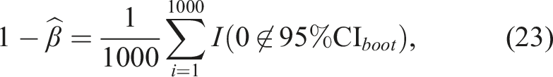
Note that making inferences and constructing confidence intervals around the AUC estimate based on the composite score is not straightforward, as one needs to account for the variability of the estimated coefficients ξ. This can be accommodated by a bootstrap-based algorithm described in the following steps.

• Step 1: Resample with replacement n₀ participants from group D = 0 and n₁ participants from group D = 1. These participants (that may contain duplicates) form the ‘current bootstrap sample’.

• Step 2: Based on the current bootstrap sample from Step 1, perform the ‘combination algorithm’ presented above and obtain the optimal ξ that maximizes the AUC.

• Step 3: Using the ξ = [ξ₁, ξ₂, …, ξ _k ] obtained in Step 2, construct the ROC and obtain the corresponding AUC.

• Step 4: Repeat Steps 1–4 1000 times to obtain 1000 bootstrapped AUCs.

• Step 5: Report the (1 − a)%CI for the AUC by obtaining the α/2 − th percentile and the 1 − α/2 − th percentile of the obtained 1000 AUC values of Step 4.

There are other alternative approaches that result in linear combinations and utilize different objective functions such as the Youden index. ²¹ Other investigators have also focused on linear combinations of markers and consider maximizing the AUC (see Pepe et al. ²² Liu et al. ²³ ). A review as well as a comparison between these methods is provided in Yan et al. ¹⁷

Assessing the risk of a favorable versus an unfavorable outcome at baseline - link of the ROC and the logistic regression model

We will explore two strategies for the assessment of the risk of an individual at baseline. One is determined by the well known logistic regression model and one is based on the modeling presented in the previous subsection. For the former, we have the usual formulation

$\mathit{l}\mathit{o}\mathit{g}\mathit{i}\mathit{t}\left(P\left(D_i=1|Y_i=y,Z_i=z\right)\right)={\theta }_0+{\theta }_1{Y}_i+{\theta }_2{Z}_i$

(15)

Such a formulation allows us to explore the risk of an unfavorable outcome given the biomarker value at baseline and the baseline profile. A unit increase of the biomarker Y implies an increase θ₁ of the logarithm of the odds ratio, when everything else (here Z) remains unchanged. Exploring the probability of an unfavorable outcome by utilizing the cutoff discussed in the previous subsection implies the modified formulation

$\begin{array}{c}\mathit{l}\mathit{o}\mathit{g}\mathit{i}\mathit{t}\left(P\left(D_i=1|Y_i>c^{*},Z_i=z\right)\right)={\theta }_0+{\theta }_{1}I\left(Y_i>c^{*}\right)\\ +{\theta }_2{Z}_i\end{array}$

(16)

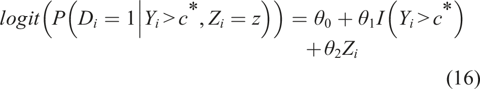
This model of log-odds given the biomarker and the baseline characteristics depends on the pre-test probability of an unfavorable outcome (i.e. the marginal probability of P(D = 1) (or overall risk), known also as the prevalence in a diagnostic testing setting). Models (15) and (16) can be easily extended to include multiple covariates (Z).

An alternative strategy, that also depends on the pre-test probability P(D = 1), is to move forward by accounting the Cox-modeling utilized to evaluate the biomarker’s performance. Such a strategy implies that (under the Bayes’ rule)

$\begin{array}{cc}P\left(D=1|Y>c,Z=z\right)& =\frac{P\left(Y>c,Z=z|D=1\right)P\left(D=1\right)}{{\sum }_{i=0}^{1}P\left(Y>c,Z=z|D=i\right)P\left(D=i\right)}\\ & =\frac{P\left(Y>c|Z=z,D=1\right)f\left(z|D=1\right)P\left(D=1\right)}{{\sum }_{i=0}^{1}P\left(Y>c|Z=z,D=i\right)f\left(z|D=i\right)P\left(D=i\right)}\\ & =\frac{S_1\left(c|Z=z\right)f\left(z|D=1\right)P\left(D=1\right)}{{\sum }_{i=0}^1{S}_i\left(c|Z=z\right)f\left(z|D=i\right)P\left(D=i\right)}\end{array}$

(17)

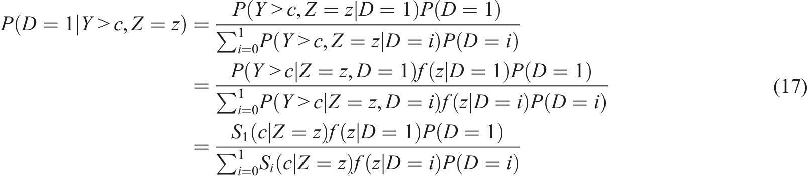
The quantities S _i (c|Z = z), i = 0, 1, can be determined based on model (4) and P(D = 1) refers to the pre-test probability of an unfavorable outcome that we assume is given by subject matter experts. In the case of a single continuous covariate, Z, for obtaining P(Z = z|D = i), i = 0, 1, one can consider parametric or non-parametric modeling such as kernel density estimation in case Z is continuous. However, this approach becomes computationally intensive when multiple covariates (Z) are present.

Note that, in the discussed study (data), an important covariate is the so-called time to measurement. Even if all subjects released biomarkers at the same rate after injury, the time from injury to baseline measurement varies enough between subjects. This variable can be straight-forwardly accommodated as a covariate in Z.

Link of the logistic regression and the ROC

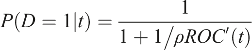
As discussed above, a usual approach that many investigators use to assess the discriminatory ability of a biomarker is the ROC, and similar to the logistic regression, it usually involves two variables: the value of a continuous marker (r.v. Y) and the disease status (or outcome) that is binary D = 0 or 1. Assume Y|D = d ∼ F _d , d = 0, 1, and D ∼ Bernoulli(π). The pre-test risk of an unfavorable outcome is denoted by π. This is translated as the probability that a TBI patient exhibits an unfavorable outcome without having the knowledge of the biomarker values. We denote the pretest outcome odds by ρ and the density ratio (or likelihood ratio) by r(). The post-test risk of (an unfavorable) outcome is the probability of an unfavorable outcome given the value of the marker, P(D = 1|Y = y). Using Bayes theorem we have

$\begin{array}{cc}\mathit{l}\mathit{o}\mathit{g}\mathit{i}\mathit{t}\left(P\left(D=1|Y=y\right)\right)& =\ln \left(\frac{P\left(D=1|Y=y\right)}{P\left(D=0|Y=y\right)}\right)\\ & =\ln \left(\frac{\pi }{1-\pi }\right)+\ln \left(\frac{f_1\left(y\right)}{f_0\left(y\right)}\right)\\ & =\ln \hspace{0.17em}\rho +\ln \hspace{0.17em}r\left(y\right)\end{array}$

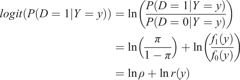
We note here that the post-test risk of an unfavorable outcome is a monotone function of the density ratio. Since the density ratio transformation yields the optimal ROC, so does the predicted (post-test) risk. Moreover, since only the intercept is affected by π, use of the estimated predicted probabilities from a logistic regression where the sample pre-test risk is a non-consistent estimate of the true pre-test risk (π) will yield a valid estimate of the optimal ROC, when the form of the density ratio is correctly specified. These facts are commonly utilized in the machine learning community.

By referring to the value of the marker as the upper t quantile of the healthy distribution $S_0^{-1}\left(t\right)$ , with t being the false positive rate, we can write

$\begin{array}{cc}\ln \left(\frac{P\left(D=1|t\right)}{P\left(D=0|t\right)}\right)& =\ln \hspace{0.17em}\rho +\ln \hspace{0.17em}r\left(S_0^{-1}\left(t\right)\right)\\ & =\ln \hspace{0.17em}\rho +\ln \hspace{0.17em}\mathit{R}\mathit{O}{\mathit{C}}^{\prime }\left(t\right)\end{array}$

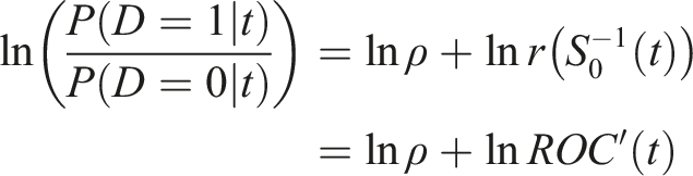
Note that when operating at a false positive rate t, the post-test odds of disease is ROC′(t) times the pretest odds of an unfavorable outcome. The post-test risk of disease is obtained as

$P\left(D=1|t\right)=\frac{1}{1+1/\rho \mathit{R}\mathit{O}{\mathit{C}}^{\prime }\left(t\right)}$

Note that for proper (i.e. concave) ROC curves the post-test risk is maximized at t = 0. For markers that correspond to improper ROC curves, this may not be the case.

Longitudinal analysis for assessing the predictiveness (or prognostic value) of the biomarkers - GEE versus mixed modeling

Exploring the time-dependent trajectory of the biomarkers through GEE

This section involves exploring the longitudinal trajectory of each marker and how it is affected by the different doses/treatment of HBOT. Namely, we first consider exploring the predictiveness of the biomarkers, since we are associating their trajectory with the treatment. Note that doses/treatment is considered as a discrete random variable. In our study, samples of whole blood will be collected every 8 h during the first 24 h post-enrollment. On study days 2, 3, 5, 7, 14 and 180, blood will be collected once a day. To assess the biomarkers’ time-trajectories we utilize marginal models under a GEE framework. 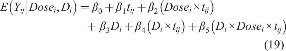As mentioned in Fitzmaurice, ²⁴ the term marginal indicates that the model for the mean response depends only on the covariates of interest, and not on any random effects or previous responses. Namely, the marginal model does not incorporate individual-specific random effects that are used in the mixed modeling modeling approach that we discuss in the next section. An appealing characteristic in the GEE is that we do not need any strict parametric assumptions for the error term, as opposed to a mixed model strategy that typically relies on multivariate normal assumptions. Under the GEE approach the trajectory of a biomarker Y conditioned on the treatment (or say level of Dose) and D (favorable (D = 0) or unfavorable outcome (D = 1)) is

$\begin{array}{c}{Y}_t|\mathit{D}\mathit{o}\mathit{s}\mathit{e},D={\beta }_0+{\beta }_{1}t+{\beta }_2\left(\mathit{D}\mathit{o}\mathit{s}\mathit{e}\times t\right)+{\beta }_{3}D\\ +{\beta }_4\left(D\times t\right)+{\beta }_5\left(D\times Dose\times t\right)+{ϵ}_t\end{array}$

(18)

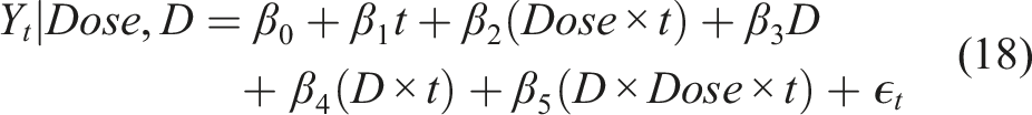
Such a model implies that at baseline (t = 0):

• If D = 0 we have: E(Y _t |Dose, D) = β₀,

• If D = 1 we have: E(Y _t |Dose, D) = β₀ + β₃.

This formulation implies that within a specific group (D = 0 or D = 1) we have a common intercept at baseline (either β₀ or β₀ + β₃, regardless of the dose level) which is a natural assumption. In addition, the difference in baseline is common for favorable and unfavorable outcomes which is also a natural assumption. At time t we have:

• If D = 0 and Dose = 0 we have: E(Y _t |Dose, D) = β₀ + β₁t,

• If D = 0 and Dose = 1 we have: E(Y _t |Dose, D) = β₀ + (β₁ + β₂)t,

• If D = 1 and Dose = 0 we have: E(Y _t |Dose, D) = (β₀ + β₃) + (β₁ + β₄)t,

• If D = 1 and Dose = 1 we have: E(Y _t |Dose, D) = (β₀ + β₃) + (β₁ + β₂ + β₄ + β₅)t.

We do not include the Dose as a main effect since individuals are randomly assigned to different dose levels.

Re-writing model (18) in terms of the available data we have

$\begin{array}{c}E\left(Y_{ij}|\mathit{D}\mathit{o}\mathit{s}{\mathit{e}}_i,D_i\right)={\beta }_0+{\beta }_1{t}_{ij}+{\beta }_2\left(\mathit{D}\mathit{o}\mathit{s}{\mathit{e}}_i\times t_{ij}\right)\\ +{\beta }_3{D}_i+{\beta }_4\left(D_i\times t_{ij}\right)+{\beta }_5\left(D_i\times \mathit{D}\mathit{o}\mathit{s}{\mathit{e}}_i\times t_{ij}\right)\end{array}$

(19)

where index i refers to the i − th individual and index j refers to the j − th timepoint. Note that depending on the behavior of the data one can easily consider higher order terms (i.e. have a polynomial or even a spline-based structure) to allow for more flexibility as well as interactions with time when clinically suitable. When such a flexibility is allowed, trajectories may be non-linear over time and a graphical example is given in Figure 1. In that simulated plot we illustrate the trajectory of a marker for different dose levels of HBOT over time as well as for different groups (D = 0 or D = 1).

Figure 1.

Time-dependent trajectory of a hypothetical biomarker for different doses of HBOT and for different groups (D = 0 or D = 1). For a given biomarker, if favorable and unfavorable outcomes have separate trajectories, but dose one and dose two have the same trajectories, the markers are prognostic but not predictive. If dose one and dose two have different trajectories, but good and bad outcomes do not, then it is a response biomarker, but not predictive.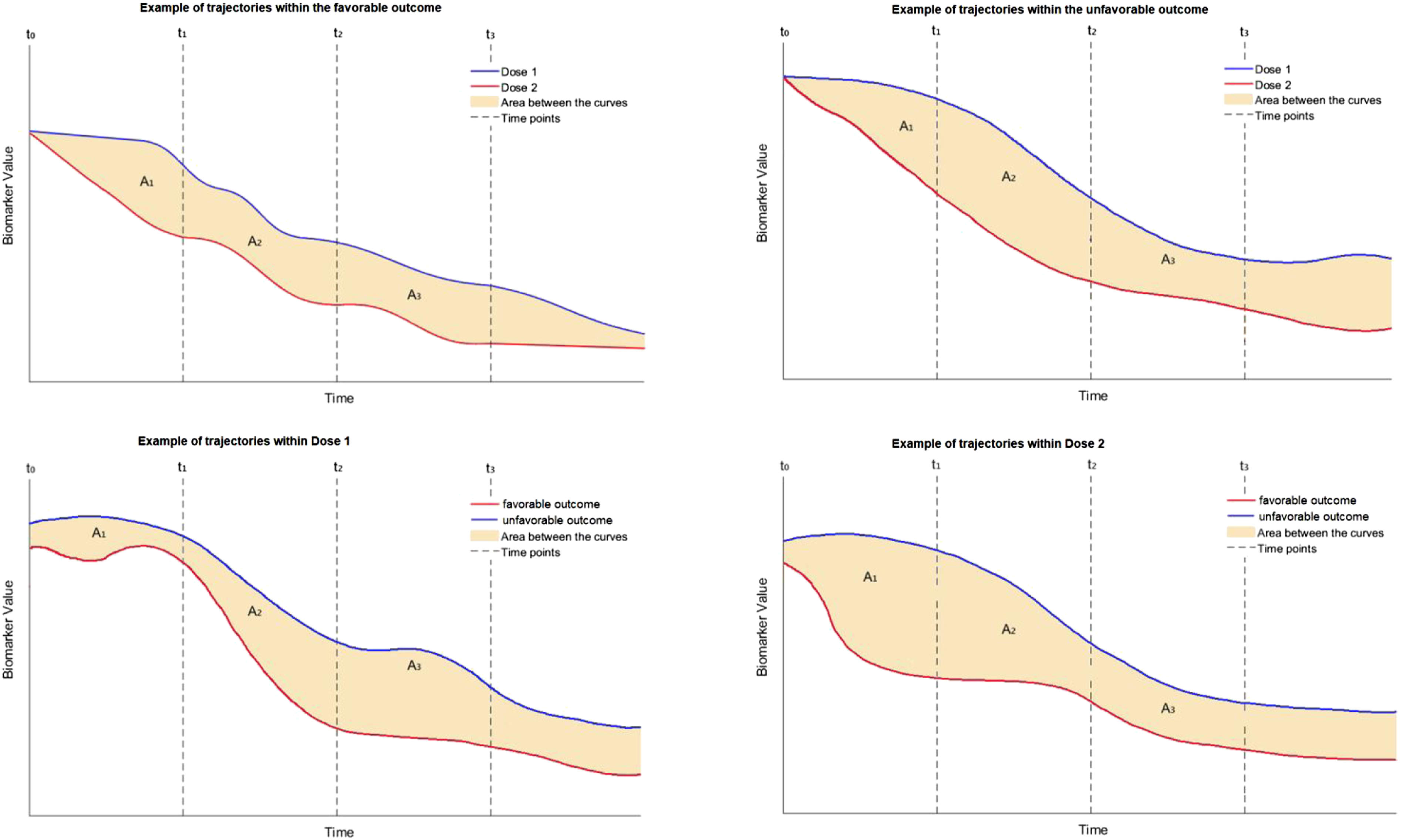

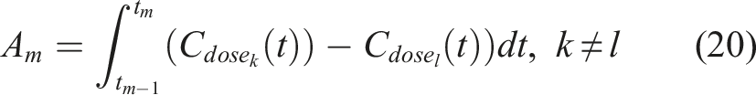
The estimation of the coefficients involved in (18) can be done through an iterative process called iterative re-weighted least squares (IRLS) within the GEE framework, and nowadays this process is automated by many statistical software packages. The trajectory of each marker can be visualized accordingly for any given profile or any given dose of HBOT (see Figure 1 for a hypothetical example). The comparison of the levels of a single biomarker for different levels of doses at a given baseline profile can be based on the area between the two trajectories, either for the whole time-period of the study, or at a given time-interval of interest. This might involve consecutive timepoints [t_m−1, t _m ]. The comparison of the two curves for a given time-interval [t_m−1, t _m ] can be assessed by

$A_m={\int }_{t_{m-1}}^{t_m}(C_{\mathit{d}\mathit{o}\mathit{s}{\mathit{e}}_k}(t))-C_{\mathit{d}\mathit{o}\mathit{s}{\mathit{e}}_l}(t))dt,k\ne l$

(20)

where $C_{\mathit{d}\mathit{o}\mathit{s}{\mathit{e}}_k}\left(t\right)=E\left(Y_t|\left(\mathit{D}\mathit{o}\mathit{s}\mathit{e}=\mathit{d}\mathit{o}\mathit{s}{\mathit{e}}_k,Z\right)\right)$ for k = 1, 2, 3, ….

Note that even though this section focuses on the predictiveness, the prognostic value of a biomarker can also be assessed in a longitudinal fashion. In a setting where there is no association with a disease (by design), one could have longitudinal measurements of a biomarker associated with an outcome (all individuals are in the same treatment - in many settings this may imply no treatment at all).

Exploring the time-dependent trajectory of the biomarkers through mixed modeling

An alternative approach to assess the trajectory of each biomarker over time is a mixed-modeling-based approach. Such an approach is different than a GEE-based approach since random effects are also incorporated in the model; a feature that provides both advantages and disadvantages. Before we point them out (see next paragraph), we refer to the structure of a plausible mixed model for this study

$\begin{array}{c}E\left(Y_{it}|\left(\mathit{D}\mathit{o}\mathit{s}{\mathit{e}}_i,t\right);b_i\right)={\beta }_0+{\beta }_{1}t+{\beta }_2\left(\mathit{D}\mathit{o}\mathit{s}{\mathit{e}}_i\times t\right)\\ +{\beta }_3{D}_i+b_{0i}+b_{1i}t\end{array}$

(21)

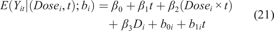
In the simplest case with two levels of dose, this model implies that the subject specific mean at time t is:

• For status D = 0 and Dose = 0 then (β₀ + b_0i) + (β₁ + b_1i)t

• For status D = 0 and Dose = 1 then (β₀ + b_0i) + (β₁ + β₂ + b_1i)t

• For status D = 1 and Dose = 0 then (β₀ + β₃ + b_0i) + (β₁ + b_1i)t

• For status D = 1 and Dose = 1 then (β₀ + β₃ + b_0i) + (β₁ + β₂ + b_1i)t

Such a model incorporates the random effects (b_0i, b_1i). This formulation implies that each participant is allowed to have their own personalized intercept (β₀ + b_0i) and their own slope (β₁ + b_1i) over time for D = 0 and Dose = 0. These slopes and intercepts change for any combination of D and Dose as shown above. That is, we have a separate regression line for each individual, which allows us to better explore the individual specific trajectories over time (and not just explore the average/marginal trajectory as in the GEE approach). However, a mixed modeling approach implies some parametric assumptions for the extra random effects. These random effects are usually assumed to follow a multivariate normal distribution. The mixed model approach requires a larger sample size (compared to the GEE) in order to efficiently estimate the parameters of the multivariate distribution. This is due to the larger number of parameters to be estimated. The GEE approach does not need such parametric assumptions and has been shown to be robust even under miss-specification of the error terms (the so called ‘sandwich estimator’ of the GEE framework is quite robust even under a miss-specified underlying correlation matrix). An advantage of the mixed modeling approach is that the accommodation of exogenous time-dependent covariates is straightforward, as opposed to a GEE-based approach. Another advantage of the mixed modeling approach over the GEE, is that it yields subject specific predictions that can be valuable in some settings. We note that both the GEE and the mixed modeling approach are available in roentgen and MATLAB. ²⁵

Simulation section

Our simulations are reported in two parts. One that refers to the baseline performance of the markers and one that refers to the longitudinal analysis and their time-dependent behavior. More specifically, for the first part we assess the expected accuracy of a combination of three biomarkers under several scenarios when these are combined using the 5-Step algorithm previously described. For the second part we explore the power and size that refers to assessing the significance of the areas A _m . In addition, we explore the bias, the variance, and the MSE of the ${\widehat{A}}_m$ for several scenarios.

Combinations of markers at baseline

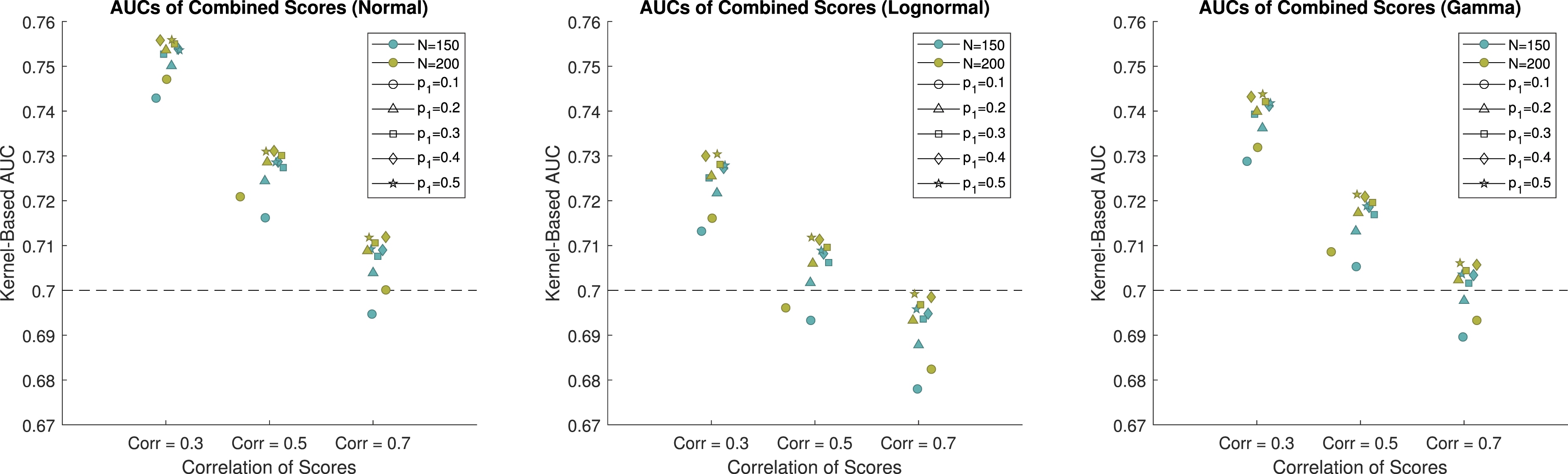
For the simulation study, we consider combining three biomarkers into a single pseudoscore to achieve higher discriminatory ability than any individual biomarker that is collected in the study. The biomarker scores were simulated from normal, lognormal, and gamma distributions in order to demonstrate the performance of Yan’s method ¹⁷ in a wide variety of scenarios. The AUC is a measure of the performance of a biomarker. A properly ordered biomarker will have values ranging from 0.5 to 1. For the simulation study we considered individual biomarkers with AUCs of 0.7, which is indicative of a moderately useful biomarker. The sample size of the study is 200, but dropout is expected to be as high as 25%, and therefore sample sizes of 200 and 150 were used for this simulation study. The number of participants who will achieve a positive outcome is unknown, and therefore we use allocation proportions of 0.1, 0.2, 0.3, 0.4, and 0.5 to cover a reasonable set of scenarios for the proportion of participants who achieve a positive outcome. Additionally, the biomarkers being explored in this study are expected to be correlated, and thus, we consider markers with correlations of 0.3, 0.5, and 0.7, to cover low, medium, and high correlations for the markers to be combined. The combined score for each of the scenarios was evaluated using both the kernel-based and the empirical estimate of the AUC on an independent testing dataset, where the sample size for both groups was 10,000. Using an independent testing dataset of a high sample size allows us to gauge how the combined score would perform in the population, rather than just in the sample at hand. It is important to evaluate the results from independent data in order to avoid overfitting that is seen when only looking at training data.

When the biomarkers are simulated from normal distributions and the sample size is 150, the estimated AUCs for the combined score range from 0.6964 to 0.7539. Results for the normal scenarios are displayed in Figure 2, 3 and Table 1 of the Web Appendix. The method performs poorly when the allocation of subjects to each group is highly unbalanced, and it performs better when the allocation of subjects is balanced. When the correlation is equal to 0.7, the combination struggles to achieve an AUC that is higher than 0.7. When only 10% of the subjects achieve a positive outcome, the combined score had an estimated AUC of 0.6964, which is below the AUC of the individual markers. At best, when the correlation is 0.7, the combined score achieved an estimated AUC of 0.7111, which is 0.0111 higher than the individual biomarkers. This demonstrates minimal improvement over the individual scores. When the correlation is equal to 0.3, the combined score achieves an estimated AUC between 0.7181 and 0.7539. This shows that when the biomarkers have low correlation, it is possible to achieve better performance than the individual scores. When the sample size is 200, we see improved performance compared to when the sample size is 150. In all instances, the estimated AUC of the combined score is above 0.7. When the correlation is equal to 0.7, the combined score achieved an estimated AUC between 0.7019 and 0.7138. Again, this demonstrates that combinations of biomarkers with high correlations struggle to provide additional information compared to the individual markers. When the correlation is equal to 0.3, the combined score achieved an estimated AUC between 0.7492 and 0.7580. This corresponds to an AUC that is between 7.0% and 8.3% higher than the individual markers, depending on the proportion of subjects who achieved a positive outcome.

Figure 2.

The kernel-based estimates of the AUCs of the combined scores when the data are generated from normal distributions. The individual scores each have an AUC of 0.7.

Figure 3.

The empirical-based estimates of the AUCs of the combined scores when the data are generated from normal distributions. The individual scores each have an AUC of 0.7.

When the biomarkers are simulated from lognormal distributions and the sample size is 150, the estimated AUCs are between 0.6809 and 0.7308 (results for the lognormal distributions are presented in Table 1 of the Web Appendix). Again, we see that as the correlation between the biomarkers increases, the AUC of the combined marker is smaller. When the correlation is 0.7, the combination failed to outperform the individual biomarkers, with the highest AUC being 0.6988. When the correlation is 0.3, the estimated AUCs range from 0.7171 to 0.7308. This again shows that when the sample size is 150, the benefit from combining biomarkers is limited. When the sample size is 200, the estimated AUCs are between 0.6853 and 0.7333. This shows only minor improvement compared to when the sample size is 150.

When the biomarkers are simulated from gamma distributions and the sample size is 150, the estimated AUCs are between 0.6922 and 0.7445 (results for the gamma distributions are presented in Tables 2 and 3 of the Web appendix). When the correlation was equal to 0.7, the combined score provided an AUC of 0.7062 when the sample sizes were not equal. This is not a substantial improvement over the individual scores. When the correlation was equal to 0.3, the pseudoscore saw an AUC that was between 4.9% and 6.4% higher than the individual markers. When the sample size is 200, the estimated AUCs are between 0.6959 and 0.7465. This demonstrates only minor improvement above when the sample size was 150. We see that when the correlation is 0.7 and the percent of participants with a positive outcome is 10%, the estimated AUC is 0.6959, which is lower than the individual marker AUCs of 0.7. When the correlation is equal to 0.3, and the percent of participants with a positive outcome is 50%, the estimated AUC is 0.7465. This corresponds to an AUC that is 6.6% higher than the individual markers.

In summary, the performance of the pseudoscore is highly dependent on the correlation of the biomarkers, as well as the proportion of participants who saw positive outcomes. When the scores are generated from normal distributions, the sample size also played a large role in the performance of the pseodoscore. For the scenarios generated from lognormal or gamma distributions, the sample size appeared to play less of a role in the performance of the combined score, although the scenarios with sample sizes of 200 provided higher AUCs than the corresponding scenarios where the sample size was 150. Lower correlations and a more even sample size for positive/negative outcomes led to higher estimated AUCs. When the correlation was equal to 0.7, the pseudoscore struggled to outperform the individual markers in all scenarios, and was frequently below 0.7, and was as low as 0.6853.

Time trajectory of the biomarkers through GEE to compare two dose levels

Reduced model

To evaluate this method for the time-dependent trajectory of a biomarker between two dose levels, we considered a model for the first four timepoints that are equally spaced. For illustration purposes we focus on the unfavorable outcome group and consider a model to detect dose effects (analogous to focusing only on the setting presented in the top-right panel of Figure 1). For the sake of simplicity we consider only two doses, with various sample sizes, to explore the power for detecting A₁ (see Figure 1) as statistically significant. The dose effect is summarized by A₁, A₂, …, and dose effects for both favorable and unfavorable outcomes can be estimated from the full model that includes the status D as shown in equations (18) and (19). Multiple dose levels can be accommodated using dummy variables. The reduced model (within the unfavorable outcome group) we focus on during this part of simulations is of the form

$E\left(Y_{ij}|\mathit{D}\mathit{o}\mathit{s}{\mathit{e}}_i\right)={\beta }_0+{\beta }_1{t}_{ij}+{\beta }_2\left(\mathit{D}\mathit{o}\mathit{s}{\mathit{e}}_i\times t_{ij}\right)$

(22)

where Dose _i = 0, one and t _ij = 0, 8, 16, 24. We studied the variance, power, coverage probabilities, and biases for the area between the two dose curves within the first interval t = [0, 8], denoted by A₁. Where A₁ is defined in (18) for m = 1, k = 1, and l = 0.

We evaluated A₁ at various sample sizes and true A₁ values. Sample sizes for Dose 0 and Dose 1 (n₀, n₁) were chosen as: (14, 14), (20, 20), (30, 30), (40, 40), (50, 50), and (130, 26) (with the last sample sizes being plausible/expected based on the resources and recruitment for our study). True values of β were first chosen to obtain an A₁ value of 0.4. We then increased the value of A₁ by 0.05 for each simulation until a power of 0.8 was obtained.

We ran 1000 Monte Carlo simulations to estimate the variance, bias, coverage probability, confidence interval width, and power. For each iteration, we simulated values of the response variable y at each timepoint for the specified number of subjects in each dose group. Values were generated using values of β that yielded the specified A₁ values and adding error terms. The error terms were randomly generated for each subject from a multivariate normal distribution with a standard deviation of one and a covariance of 0.6 between timepoints. We then fit the GEE model (22) using the simulated data.

Using the estimated values of β, we calculated A₁ using the trapezoidal rule. Variances and 95% confidence intervals of A₁ were estimated using 1000 bootstrap iterations. Using the bootstrap estimated 95% confidence intervals, we estimated the power using the expression

$\begin{array}{c}1-\widehat{\beta }=\frac{1}{1000}{\displaystyle \sum }_{i=1}^{1000}I\left(0\notin 95\%{\mathrm{C}\mathrm{I}}_{\mathit{b}\mathit{o}\mathit{o}\mathit{t}}\right),\end{array}$

(23)

The Monte Carlo estimates, variance, MSE, power, coverage probability, and width of the 95% confidence interval for A₁ are shown in Tables 4 and 5 of the Web Appendix. The power for A₁ at all simulated values of A₁ are shown by sample size in Figure 4. The biases for A₁ remained somewhat constant for varying true values and sample sizes. The biases for A₁ ranged from −0.04,051 to 0.0243. The coverage probabilities for A₁ were all close to 0.95, and did not increase significantly with increases in sample size or true value. The variances decreased as sample size increased, but did not change significantly with changes in true A₁ values.

Figure 4.

Power results for a simulation regarding the bootstrap-based inference around A₁. Simulations were generated for each sample size starting at A₁ = 0.4 and increasing by 0.05 until a power of at least 0.8 was achieved for A₁. We explored equal sample sizes of (14, 14), (20, 20), (30, 30), (40, 40), and (50, 50) and an unequal sample size of (130, 26).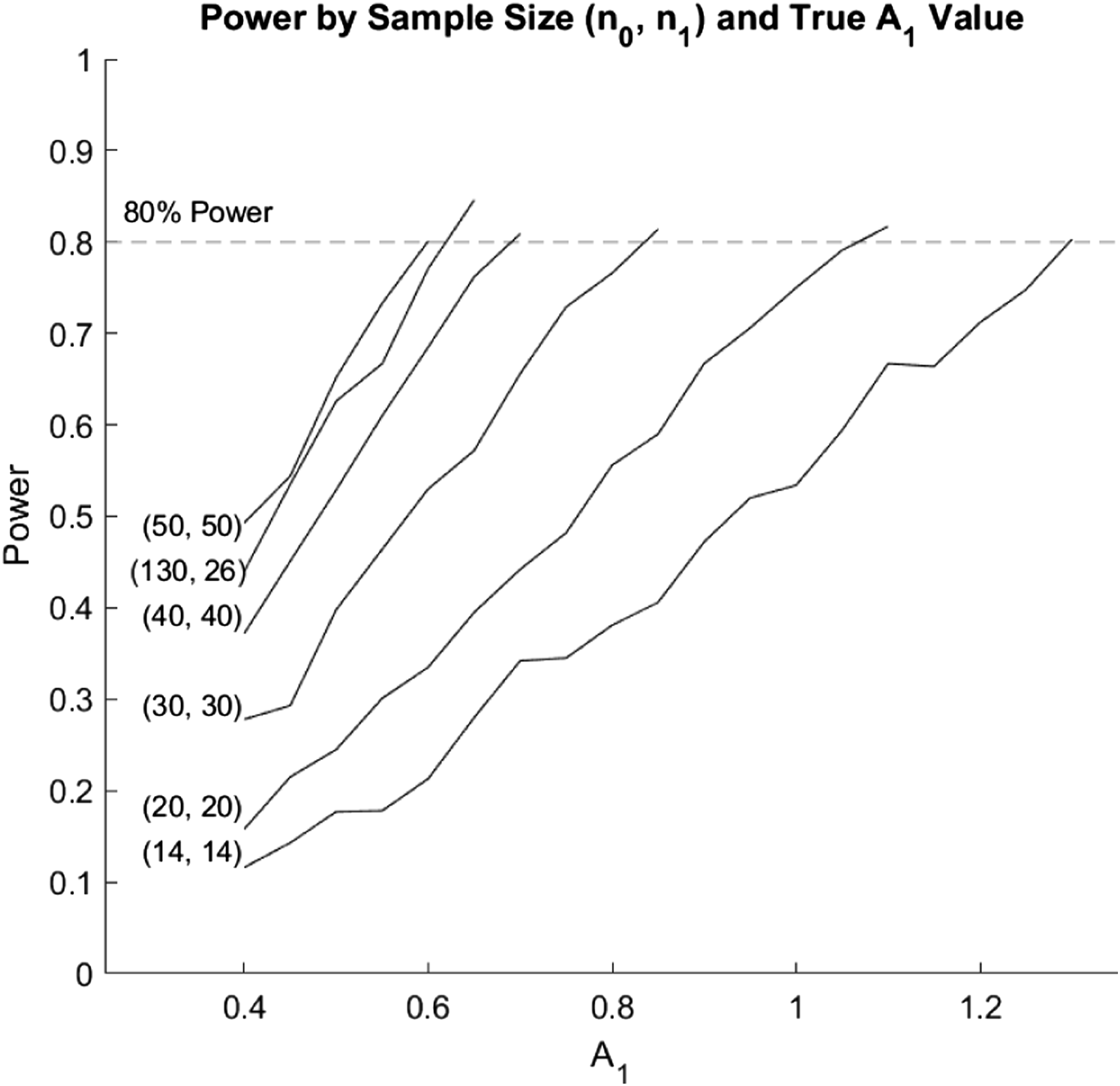

The power for A₁ tended to increase with increases in sample size when both treatment groups had equal sample sizes. However, unequal samples resulted in lower power. Although the sample size of (130, 26) had a much higher total sample size compared to (50, 50), the (50, 50) sample size still performed better across all values of A₁. Additionally, the power tended to increase as the true values of both variables increased. However, power tended to increase at a slower rate for lower sample sizes compared to the higher sample sizes. Therefore, if an investigator expects an A₁ value of 0.6, a sample size of at least 50 in each dose group would be required to obtain 80% power. For an expected A₁ value of 0.7, a sample size of at least 40 in each dose group would be required to obtain 80% power. An expected A₁ value of 0.85, 1.1, and 1.3 would require at least 30, 20, and 14 subjects in each dose group, respectively to obtain 80% power. However, if the sample size is unbalanced between the two dose groups, a higher total sample size will be required.

Full model

We also considered the full model (18) in evaluating the time trajectory of the biomarkers among those with a favorable outcome and those with an unfavorable outcome between two dose levels. We considered the outcome at two doses levels with various sample sizes, to explore the power for detecting A₁₁ − A₀₁, where A₁₁ is the area between the biomarker trajectories at the first timepoint for those with an unfavorable outcome compared to those with a favorable outcome at Dose level 1 and A₁₀ is the area between the biomarker trajectories for those with an unfavorable outcome compared to those with a favorable outcome at Dose level 0. This is illustrated in Figure 1 where A₁₁ − A₀₁ is the difference in A₁ areas in the lower two panels for dose levels of 0 and 1.

We ran 1000 Monte Carlo simulations to estimate the variance, bias, coverage probability, confidence interval width, and power of A₁₁ − A₀₁ for the following sample sizes ((n₀, n₁)): (130, 18), (130, 20), and (130, 30). To calculate the size of the test, we used values of β that yielded a true difference of 0 to test the null hypothesis of A₁₁ − A₀₁ = 0. To calculate the power, we used values of β that yielded true differences of 1 through 2.8. For the n₀ subjects who received dose 0, we assumed a probability of a favorable outcome of 0.2, and for the n₁ subjects who received dose 1, we assumed a probability of a favorable outcome of 0.3. For each iteration, we randomly assigned a favorable or unfavorable outcome to each subject based on these probabilities. We then generated biomarker values using values of β chosen to achieve A₁₁ − A₀₁ values of 0, and 1 through 2.8. Error was added for each subject by randomly generating values from a multivariate normal distribution with means of 0, variances of 1, and covariances between timepoints of 0.6. We then fit the full GEE model given in (18) and calculated the differences in areas between the two dose groups using the trapezoidal rule. Variances and 95% confidence intervals of the areas were calculated using 1000 bootstrap iterations. Power was calculated using equation (23).

The Monte Carlo estimates, variance, MSE, power, size, coverage probability, and width of the 95% confidence interval for A₁₁ − A₀₁ are shown in Table 6 of the Web Appendix and the power is shown in Figure 5. The biases remained relatively constant with increases in both the true difference and n₁, and ranged from −0.0362 to 0.0265. The coverage probabilities were all close to 0.95, and did not increase significantly with increases in sample size or true value. Additionally, the variances decreased as sample size increased. At the highest sample size (130, 30), the variance did not change significantly with changes in true differences. However, for the two lower sample sizes, the variance tended to increase as the true difference increased. The estimated size of the test of the differences was close to 0.05 for all three sample sizes. The power tended to increase with increases in the sample size for dose 1 (n₁), and the power tended to increase at a similar rate for all three sample sizes. A sample size of at least 30 in the Dose 1 group would be required to obtain 80% power, for detecting a difference of 1.6. A sample size of at least 20 is required to detect a difference of 2.0 with the same power. A sample size of 18 is adequate for detecting a difference of 2.4.

Figure 5.

Estimated power and variance for a simulation regarding the bootstrap based inference around A₁₁ − A₀₁. Simulations were generated for each sample size starting for true values of one through 2.8. We explored equal sample sizes of (130, 18), (130, 20), and (130, 30).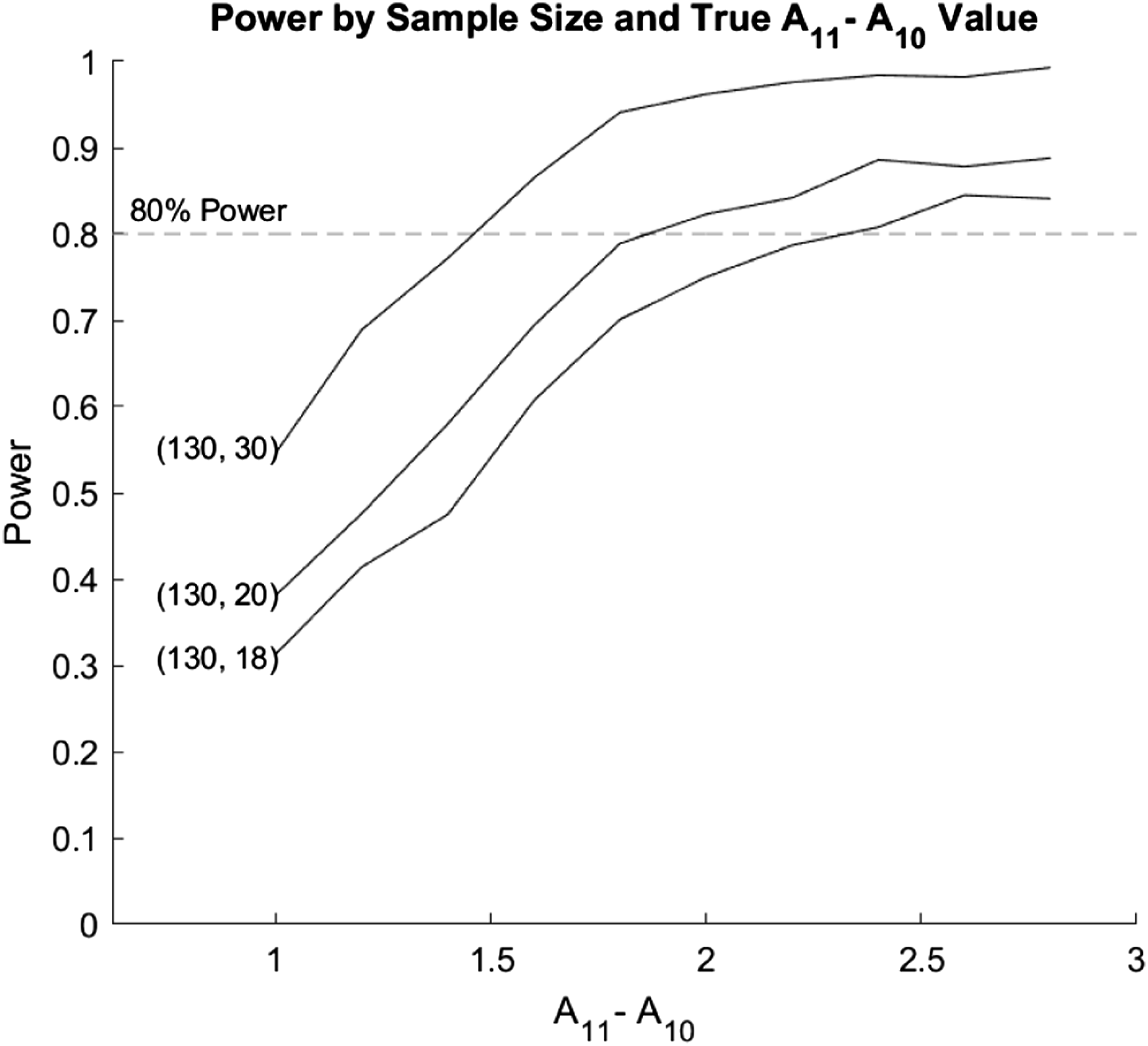

Discussion

Our motivating clinical trial and data sets focuses on the patients with severe TBI. A question that needs to be investigated is whether the Total brain tissue hypoperfusion exposure is associated with biomarkers of astrocytic (GFAP) and axonal (UCH-L1, total Tau and NF-L) injury. The behavior of these biomarkers needs to be explored in view of allowing investigators for prognostic and predictive purposes. The HOBIT trial will also allow us to explore and compare different doses of HBOT for TBI. Assessing the involved comparisons and biomarker performance involves a variety of different statistical techniques and methods that operate under different assumptions which we discuss in this paper.

Biomarker studies that refer to prognostic and predictive biomarkers are often described in the literature. Even though statistical methodologies are available for specific settings that include prognostic and predictive biomarkers, a comprehensive framework of biomarker data analysis for such studies is not readily available. In this paper we discuss the integration of techniques such as ROC analysis, logistic regression, Cox modeling, combinations of biomarkers, and time-dependent modeling with the purpose of providing a framework of data analysis in biomarker studies that involve predictive and prognostic biomarkers. We distinguish the analysis that can be performed at baseline and present alternative approaches for accommodating covariates. We discuss the relevant ROC analysis and the underlying logistic regression model and present the link between them. We further illustrate the framework for exploring the time-dependent trajectories of the markers through the use of GEE and mixed modeling and discuss the advantages and disadvantages of each approach. We illustrate the performance of the discussed approaches through extensive simulations and refer to the underlying assumptions of each. We also comment on available software/routines for applying the presented methods that can help practitioners to incorporate them to their data.

We highlight that the notions of prognosis and prediction are not mutually exclusive. A baseline marker could be prognostic at high and low levels, which could reliably predict bad and good outcomes in a manner that is not influenced at either end by exposure to the treatment. If intermediate levels were not influenced by treatment, the marker would be only prognostic. If intermediate levels led to good outcomes with treatment, but poor outcomes without treatment, the marker would also be predictive. This implies that baseline values should be explored for both prognostic and predictive uses. Similarly, repeated measures may be prognostic, predictive, both or neither, as can be seen and described in the caption of Figure 1.

An issue that is not covered in this paper refers to censored biomarker values due to limits of detection. Kernel-based imputation approaches for the construction of the underlying ROC for the whole spectrum of FPRs (even for that region that is affected by the LOD) is given in Bantis, et al. ²⁶ (the relevant routines are available at https://www.leobantis.net). We also note that the work of Cai ²⁷ and Heagerty and Pepe ²⁸ that involve a setting in which interest lies on the time-dependent sensitivity and specificity of biomarkers describes a more general framework.

Supplemental Material

Supplemental Material - Statistical assessment of the prognostic and the predictive value of biomarkers- A biomarker assessment framework with applications to traumatic brain injury biomarker studies

Supplemental Material for Statistical assessment of the prognostic and the predictive value of biomarkers- A biomarker assessment fframework with applications to traumatic brain injury biomarker studies by Leonidas E Bantis, Kate J Young, John V Tsimikas, Brian R Mosier, Byron Gajewski, Sharon Yeatts, Renee L Martin, William Barsan, Robert Silbergleit, Gaylan Rockswold and Frederick K Korley in Research Methods in Medicine & Health Sciences