Sage Journals: Discover world-class research

Abstract

Last Observation Carried Forward (LOCF) is an ad-hoc method, with known limitations. In recent years, several methods publications have used LOCF in estimating the per-protocol effect via inverse probability of adherence weighted (IPAW) model, when a time-varying factor is partially measured by the study design. We compare the statistical performances of LOCF and multiple imputation approaches for estimating the per-protocol effects via the IPAW model in the presence of incomplete treatment adherence. We used a validated pragmatic trial data generating simulation algorithm to generate datasets under 7 different simulation scenarios, where a post-randomization prognostic factor was measured after regular intervals. Unmeasured values of a partially observed factor were imputed using LOCF and multiple imputation approaches, and IPAW model was fitted on the imputed data to obtain the estimates, and statistical performances were assessed. When confounding exists, for higher variability of the time-varying factor, multiple imputation approach shows desirable statistical properties under MCAR assumption; otherwise, LOCF approach can be adequate. Both imputation methods performed well in terms of statistical properties, when there is no confounding or when all necessary confounders are adjusted. A case study from Coronary Primary Prevention Trial data was presented, which included some participants with incomplete treatment adherence.

Keywords

Adherence causal inference imputation MCAR

What is New?

What is already known

• The measurement frequency of post-randomization prognostic factors in pragmatic clinical trials is typically infrequent.

• Magnitude of bias could increase in the per-protocol estimates from the inverse probability of adherence weighted models due to the infrequent measurement of time-varying covariates.

Key findings

• When confounding exists, for higher variability of the time-varying factor, multiple imputation approaches show desirable statistical properties under MCAR assumption; otherwise, the LOCF approach can be adequate.

What this adds to what was known?

• Even when a post-randomization prognostic factor is partially unobserved due to the MCAR mechanism, the LOCF approach may not be the best approach for imputing those data points to address sparse measurement issues under certain situations.

What is the implication and what should change now?

• Variance of the post-randomization prognostic factor is an important indicator for choosing a suitable imputation method for that factor, and analysts should consider this characteristic at the statistical analysis plan stage.

Introduction

Analysis of trial data with incomplete treatment adherence

Clinical trials are considered gold-standard for regulatory decision making. For clinical decision making, pragmatic trials are helpful in answering patient-oriented questions under the real-world clinical settings that may involve heterogeneous patients. In pragmatic trials, sustained treatment strategies are often of interest. In these trials, patients are randomized to a treatment strategy at baseline, and the treatment strategy should be sustained over the follow-up for the unbiased estimation of the per-protocol effect. However, particularly when the follow-up period is long, these trial settings are more prone to incomplete adherence to the treatment.

For estimating per-protocol effects of sustained treatment strategies, naive methods such as intention to treat or naive per-protocol effect (e.g., excluding non-adherers) are known to produce biased treatment effects in the presence of incomplete adherence^1,2. As the adherence is time-dependent, researchers need to adjust for pre-randomization (baseline) covariates and post-randomization time-varying prognostic factors, which impact the treatment decisions, in order to obtain unbiased treatment effect estimates. As long as the common causes of the outcome and adherence are measured and adjusted in a correctly specified in a inverse probability of adherence weighted (IPAW) model, the estimated per-protocol effect has been shown to be asymptotically consistent³.

What is known about infrequently measured data analysis

The measurement frequency of post-randomization prognostic factors in pragmatic clinical trials is typically infrequent. A recent simulation study showed that the magnitude of bias could increase in the per-protocol estimates from IPAW models due to infrequent measurement of time-varying covariates⁴. In their simulation, measurement of adherence and time-varying covariates were taken after a certain number of months (e.g., 12 months), and for the interim months, the last measured value of the variable was imputed to make the data complete, for the estimation of the inverse probability weights. This practice of imputing unobserved values by the last observed values is known as Last Observation Carried Forward (LOCF).

Motivation and novelty of the current work

LOCF is known for its sub-optimal performance under missing at random (MAR) assumption, and multiple imputation performs better in terms of statistical properties⁵. In the literature, several published works have already investigated the statistical performance of inverse probability-weighted estimators for as-treated analyses, such as marginal structural models^6,7. Those works have considered situations where MAR assumption was more plausible, and missing completely at random (MCAR) assumption was potentially violated.

In contrast to those works, our current work focuses on a setting where sparse measurements are not due to any other extraneous factors (e.g., drop out or severe illness), but planned at the design stage. The use of LOCF approach for imputing in the infrequently measured data is not uncommon, when the missingness is unrelated to any observed and unobserved factors, but due to the planned study design. That means, for this setting, MCAR assumption may not be violated, as we are not dealing with missing data in the conventional sense, but data are observed less frequently only due to a choice of measurement frequency selected by the trial designer. Other works such as Moodie et al.⁸ considered similar sparse data conditions (e.g., data generated under MCAR: missingness is not due to or related to any patient characteristics; similar to our simulations), but also focused on as-treated analysis as in the previously mentioned works. Our work is also different from the previous works, as we are focusing on per-protocol analyses, not as-treated analysis, to deal with incomplete adherence; although all of these works are investigating the statistical performance of inverse probability-weighted estimators under different missingness mechanisms.

As a motivating example for our current work, in the Coronary Primary Prevention Trial, following the study protocol, lipid-related data were collected every 2 months, partial medical examination data were collected every 6 months, and a complete clinical history and physical examination data were collected every 12 months⁹. Note that the frequency of measurements were determined by the trial designer, and therefore the uncollected data were not due to any observed and unobserved factors. When the data was reanalyzed in recent years to estimate per-protocol effects, LOCF approach was used to impute the treatment adherence and covariate values.^10,11

Alternatives to LOCF

In general, LOCF is known to be an ad-hoc imputation method in the literature. While it helps artificially increase the amount of information for analysis by imputing the last observed value, it does not distinguish whether the values are imputed versus observed. Such a single value imputation approach potentially underestimates variances, often resulting in smaller standard errors of the estimates, and narrower confidence intervals^5,12. The problem is notably worse when the missingness follows missing at random (MAR). Even when missingness is MCAR, validity of the LOCF approach is not guaranteed in certain longitudinal trial situations¹³. When longitudinal follow up is sparse (infrequent measurements), using principled imputation approaches such as multiple imputation has been shown to reduce bias in inverse probability weighted estimator (as-treated analysis¹⁴) results compared to that from the LOCF approach¹⁵.

Given the MCAR setting, complete case analysis could be another possible strategy¹⁵. A previous simulation study estimating the per-protocol effect using IPAW model found reduced bias from complete case analyses and LOCF under MCAR assumption in an OR scale, when measurements were relatively frequent¹⁶. However, if the frequency of measurement were infrequent, many available post-randomization measurements from other variables would have to be ignored in that complete case analysis¹⁵.

Need for guideline about imputation under MCAR

Despite the known limitations of LOCF, this ad-hoc approach is still used in various trial, pragmatic trial, and target trial settings^17–19. Recent examples include pragmatic trial data analysis where per-protocol analyses were conducted via IPAW estimators^4,16,20; all of which used LOCF in their analyses. Given the warnings from statisticians, and continued use of this method in many recent advanced per-protocol analyses, it is important for the practitioners to know how the use of a particular choice of imputation approach (i.e., LOCF vs. multiple imputation) impacts the IPAW model estimates. Given the popularity and frequent usage of LOCF in estimating per-protocol effects, we have considered this method to be the focus of our investigation. Given the known benefits of multiple imputation approach (e.g., in terms of variance estimation), we have considered this method as the primary competitor. We did not consider complete case analyses as a strategy, as such method has already been compared to LOCF in a previous study estimating per-protocol effects¹⁶.

Research aim

In this work, using a validated pragmatic trial data generating simulation algorithm, we compare the relative statistical performances (e.g., reducing bias, relative precision and achieving nominal coverage) of LOCF and multiple imputation approaches for estimating the per-protocol effects via the IPAW model in the presence of incomplete adherence. We are particularly interested in situations where post-randomization prognostic factors are measured infrequently. We will illustrate the use of zip plots throughout the assessment of the simulation performances of these two imputation methods²¹. Other than simulations, we also show a case study from the Coronary Primary Prevention Trial⁹.

Methods

Notations

We have used the following notations: Z is the randomization status (binary; 1 = new treatment, 0 = comparator treatment or standard of care), U is the unmeasured risk factor of the outcome measured at baseline (continuous; generated from uniform distribution) that potentially impacts outcome as well as post-randomization prognostic factors, t is the follow-up time index, A_t is the treatment status indicator at month t (binary; whether treatment received at that month under a static treatment strategy), and Y_t+1 is the binary indicator of a health-outcome (e.g., mortality) at the end of the study. L_t represents the post-randomization prognostic factors at time t; could represent regular laboratory measurements. Two such factors were considered, L_1t (continuous; generated from normal distribution) and L_2t (binary; generated from Bernoulli distribution), and m is the measurement interval (in months) for measuring the post-randomization prognostic factor L_1t.

Data generation mechanism

We used the established and validated data generating mechanism described in Young et al.⁴ to generate pragmatic trial datasets with a survival outcome. The data generating mechanism is depicted in the diagram presented in Figure 1. In this simulation, Z (Z = 1 indicating group treated with new drug treatment; otherwise treated under standard of care) and U (unmeasured baseline factor: U_i ∼ uniform (0,1)) are generated at the beginning of the study, and the outcome Y_t+1 at the end of the study. In between, treatment status A_t and a post-randomization prognostic factor L_2t are measured on a monthly basis. For example, from health administrative data, prescription filling instances are usually recorded continuously. The other post-randomization prognostic factor L_1t (e.g., requiring going to laboratory for measurements) was measured m months apart, where possible values of m are 2, 3, 6, 12, 18, 24, 30.

Figure 1.

The data generating mechanism for the simulation study. Z = randomization, U = unmeasured baseline factor, t follow-up time, L_t = post-randomization prognostic factors at time t, A_t = treatment status at month t, and Y_t+1 = outcome.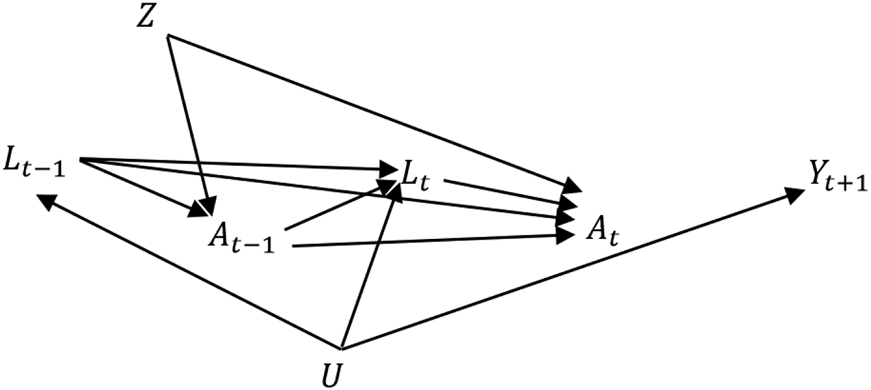

The post-randomization prognostic factors at the current period for each participant, i, were generated based on functions of previous treatment status, post-randomization prognostic factor measurements from previous time points, time index and unmeasured factor: $L_{1 t i} \sim N o r m a l (γ_{0} + γ_{1} U_{i} + γ_{2} A_{t - 1, i} + γ_{3} c u m A v g ({\bar{A}}_{t - 2, i}) + γ_{4} c u m A v g ({\bar{L}}_{1, t - 1, i}) + γ_{5} L_{2, t - 1} + γ_{6} t + ε_{i}, σ)$ , and L_2ti ∼ Bernoulli(p_L2i) where $l o g i t (p_{L 2 i}) = η_{0} + η_{1} U_{i} + η_{2} c u m A v g ({\bar{L}}_{1 t i}) + η_{3} L_{2, t - 1, i} + η_{4} A_{1, t - 1, i} + η_{5} c u m A v g ({\bar{A}}_{1, t - 2, i}) + η_{6} t$ where, cumAvg() is the cumulative average from the beginning of the follow-up to the specified time index, ${\bar{A}}_{t, i}$ and ${\bar{L}}_{t, i}$ represent treatment and covariate histories for subject $i$ respectively up to time $t$ .

For those complying with protocol, treatment status at the current period was generated as a function of A_t ∼ Bernoulli(p_Ai), where, $l o g i t (p_{A i}) = α_{0} + α_{1} c u m A v g ({\bar{L}}_{1 t i}) + α_{2} {\bar{L}}_{2, t - 1, i} + α_{3} t$ , otherwise we assume that participants remain non-compliant after deviating from the protocol for the first time. Here, α₀ can be changed for controlling the proportion of protocol deviation; but it is possible to do the same by changing γ₀, γ₁, η₀, and η₁ in certain combinations.

Finally, Y_t+1,i ∼ Bernoulli(p_Yi) where logit(p_Yi) = θ₀ + θ₁U_i. θ₀ is primarily responsible for controlling event rate, and θ₁ is the impact of the baseline factor U_i on the outcome. Parameter values for all scenarios under consideration are listed in Supplementary Table A1.

IPAW Estimator

We are primarily interested in the per-protocol effect of sustained adherence to treatment versus standard of care. The estimation of this contrast $P r (Y_{t + 1}^{\bar{a} = 1} | Z = 1)$ versus $P r (Y_{t + 1}^{\bar{a} = 0} | Z = 0)$ required following three steps^4,22. We first censored the participants at the point of protocol deviation related to treatment (i.e., first time A_t ≠ Z). We, then, calculated the IPAWs to reduce the confounding due to post-randomization prognostic factors

s w_{i t} = \prod_{j = 1}^{t} \frac{\Pr (A_{i j} | {\bar{A}}_{i, j - 1}, Z = z)}{\Pr (A_{i j} | {\bar{A}}_{i, j - 1}, L_{t}, Z = z)}

(1)

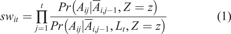
Here, both numerator and denominator can be estimated via a logistic regression model, and then cumulative products are calculated for each participant to produce stabilized weights for each month interval when the participant followed the protocol (e.g., remained uncensored). Correct specification of the denominator model is important for the consistency property of the final estimate. Finally, we estimated the measure of effects in the pseudo population using a pooled logistic regression

l o g i t (Pr (Y_{t + 1} = 1 | Z, {\bar{Y}}_{t} = 0)) = β_{0} + β_{1} Z + β_{2} t

(2)

The above working outcome model is weighted by the stabilized weights. This pooled logistic regression model is used to approximate the Cox model^23,24, and odds ratio (OR; approximating hazard ratio) is estimated using the logit link. If risk difference (RD) is of interest, identity link is used, but occasionally requires providing initial values for the parameter optimization. One can use a linear model in the latter case to avoid guessing initial values²⁵. In the presence of any baseline prognostic factor (if measured), we would incorporate that factor in the numerator and denominator of equation (1) as well as equation (2).

Imputation approaches under consideration

The first approach we considered is LOCF, which is commonly known as an ad-hoc single imputation method. Under LOCF, unmeasured observations were replaced by the subject-specific last observed values. We have considered multiple imputation models using predictive mean matching¹⁵ in the long format of the data²⁶. Multiple imputation approach first creates a predicted distribution of the variable needing imputation based on observed information, and then randomly sample to generate imputed values. This approach also deals with uncertainty by generating multiple values for the same unmeasured observation; hence creating multiple imputed datasets. For all multiple impulation applications, we used 10 imputed datasets. In the imputation models, month index (t), lag value of post-randomization prognostic factor (L_2,t−1), treatment decision in the previous month (A_t−1) were included. As we are dealing with a survival outcome, the outcome event and the Nelson–Aalen estimate of cumulative hazard were also included in the imputation model.²⁷ Results from the multiple imputed datasets were combined using Rubin’s rules.^28,29

As sensitivity analyses, we have also considered the following multiple imputation methods: (a) multilevel predictive mean matching, where each subject’s contributions were considered as a cluster, and subject ID was indicated as the cluster variable using a linear mixed model framework,³⁰ (b) random forest,³¹ (c) Bayesian linear regression and (d) linear regression.

Simulation settings considered

We considered seven settings (see Table 1). The parameter values are listed in Supplementary Table A1. In the third setting (base scenario), we has an unmeasured confounder (U), that impacted not only the outcome risk (Y_t+1), but also the treatment decision via the post-randomization prognostic factors (L_1,t, L_2,t) (see Figure 1). In this setting, L_1,t was a continuous post-randomization prognostic factor (e.g., could be laboratory measurements) generated from a normal distribution with standard deviation σ = 2 and each randomization arm consisted of 1, 000 subjects. The event rate was 20%, and proportion of protocol deviation was 40% in both arms, with moderate level of confounding in setting 3. In all of the simulations, parameter combinations were carefully chosen to keep these numbers fixed, so that the results are comparable. The data was generated up to 60 follow-up months (t = 0, …, 59), and per-protocol effect is set to null (hence, no arrows from A_t−1 or A_t to Y_t+1).

Table 1.

Simulation scenarios considered to generate pragmatic trial datasets with a survival outcome.

Scenario	n per arm	σ	Role of U
1	1, 000	0.5	Confounder
2	1, 000	3	Confounder
3 (base)	1, 000	2	Confounder
4	2, 000	2	Confounder
5	250	2	Confounder
6	1, 000	2	Risk factor for outcome
7	1, 000	5	Confounder

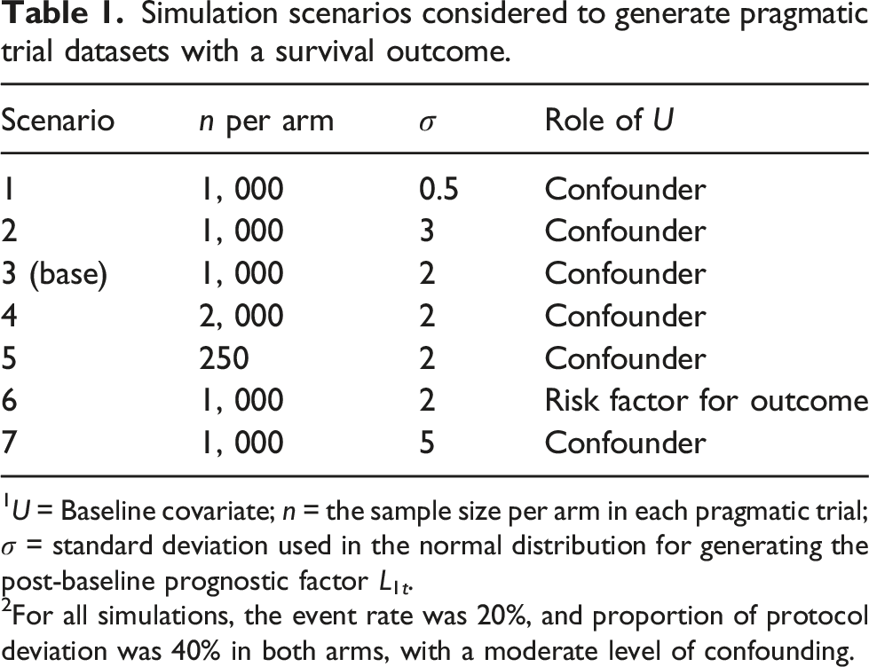
¹U = Baseline covariate; n = the sample size per arm in each pragmatic trial; σ = standard deviation used in the normal distribution for generating the post-baseline prognostic factor L_1t.

²For all simulations, the event rate was 20%, and proportion of protocol deviation was 40% in both arms, with a moderate level of confounding.

In first, second, and seventh settings, the data generating mechanism remained the same as scenario 3; but L_1,t was generated from a normal distribution with lower and higher variability (i.e., σ = 0.5, 3 and 5) respectively. Fourth and fifth settings were identical to scenario 3, except for sample size under consideration. These settings considered a larger and a smaller sample size per arm (i.e., n = 2,000 and 250) respectively. In the sixth setting, the data generating mechanism remained the same as scenario 3, with the exception that U was not a confounder any more, but just a risk factor for the outcome (Y_t+1). In this setting, U did not impact the treatment decision via the post-randomization prognostic factors.

Measures of performance

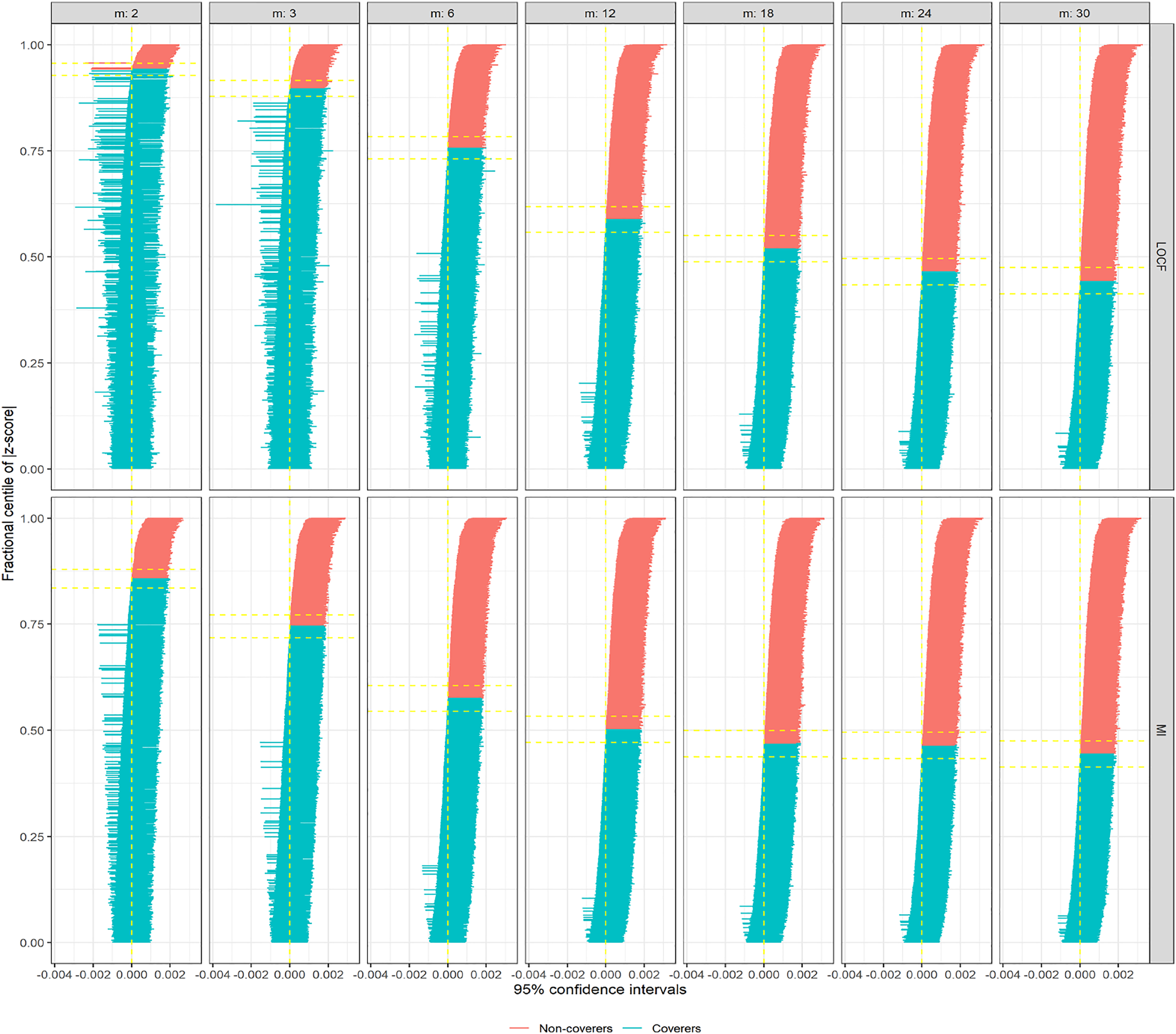
We have reported the effect measures primarily in terms of RD, although OR estimates were also calculated. We compared the results in terms of bias, average model standard error (SE), coverage of 95% confidence intervals, and bias eliminated coverage.^21,32 To understand the long term pattern of an estimator, coverage probability of 95% confidence intervals is assessed. In a frequentist sense, if 95% confidence intervals contain the parameter 95% of the times, we call it nominal coverage. Undercoverage is usually of concern, when the parameter is contained less percentage of times in the 95% confidence intervals. There can be a number of reasons for undercoverage, such as estimates are biased, model SEs being too variable, empirical SEs are greater than model SEs on an average, and wrongly assuming normality when constructing confidence intervals.²¹ To investigate the coverage in more detail, we consider zip plot, where confidence intervals are ranked by associated p-values.^21,33 R package ‘rsimsum’ was used to calculate the measures of performance.³⁴

Results

Variability of the post-randomization prognostic factor

In Figure 2, we are showing zip plots for scenario 1 (σ = 0.5). When LOCF was utilized to impute L_1t values for incremental measurement intervals (m), the coverage probabilities decrease slightly, still remaining above 90% for m = 30. In this plot, confidence intervals marked red do not cover the parameter, whereas the confidence intervals marked blue do cover the parameter. However, for multiple imputation (via predictive mean matching), the decrease in coverage probability is much more drastic, below 65% for m = 30. Comparing the Model SE and Average SE plots for this scenario, the difference was not substantial, and hence not the main reason for differential coverage probabilities between LOCF and multiple imputation (Supplementary Figures A1 and A2). However, when we investigated the bias plot, it is apparent that the bias levels from LOCF is lower than that from the multiple imputation (Supplementary Figure A3), causing the coverage probabilities also to go down for multiple imputation. The bias-eliminated coverage plot, in fact, suggested undercoverage was not an issue for LOCF or MI when bias was taken into consideration (Supplementary Figure A4). For scenario 2 (σ = 3), the apparent advantage of LOCF over MI is not so substantial anymore in terms of bias (Supplementary Figure A5); leading to the zip plots look very similar (Figure 3). For even larger σ = 5 (scenario 7), some model SEs, as well as empirical SEs from LOCF method, seemed to be associated with large variability (Supplementary Figures A6 and A7), resulting in even lower coverage probabilities for larger measurement intervals (Supplementary Figure A8).

Figure 2.

Zip plot of 1000 confidence intervals from inverse probability of adherence weighted per-protocol effect measures (in risk differences) under different measurement intervals (m, in months), comparing two imputation methods: last observation carried forward (LOCF) and multiple imputations (MI). In this generating the data for hypothetical trials (simulation scenario 1), there existed an unmeasured confounder, that induced time-dependent confounding in the process.

Figure 3.

Zip plot of 1000 confidence intervals from inverse probability of adherence weighted per-protocol effect measures (in risk differences) under different measurement intervals (m, in months), comparing two imputation methods: last observation carried forward (LOCF) and multiple imputations (MI). In this generating the data for hypothetical trials (simulation scenario 2), there existed an unmeasured confounder, that induced time-dependent confounding in the process.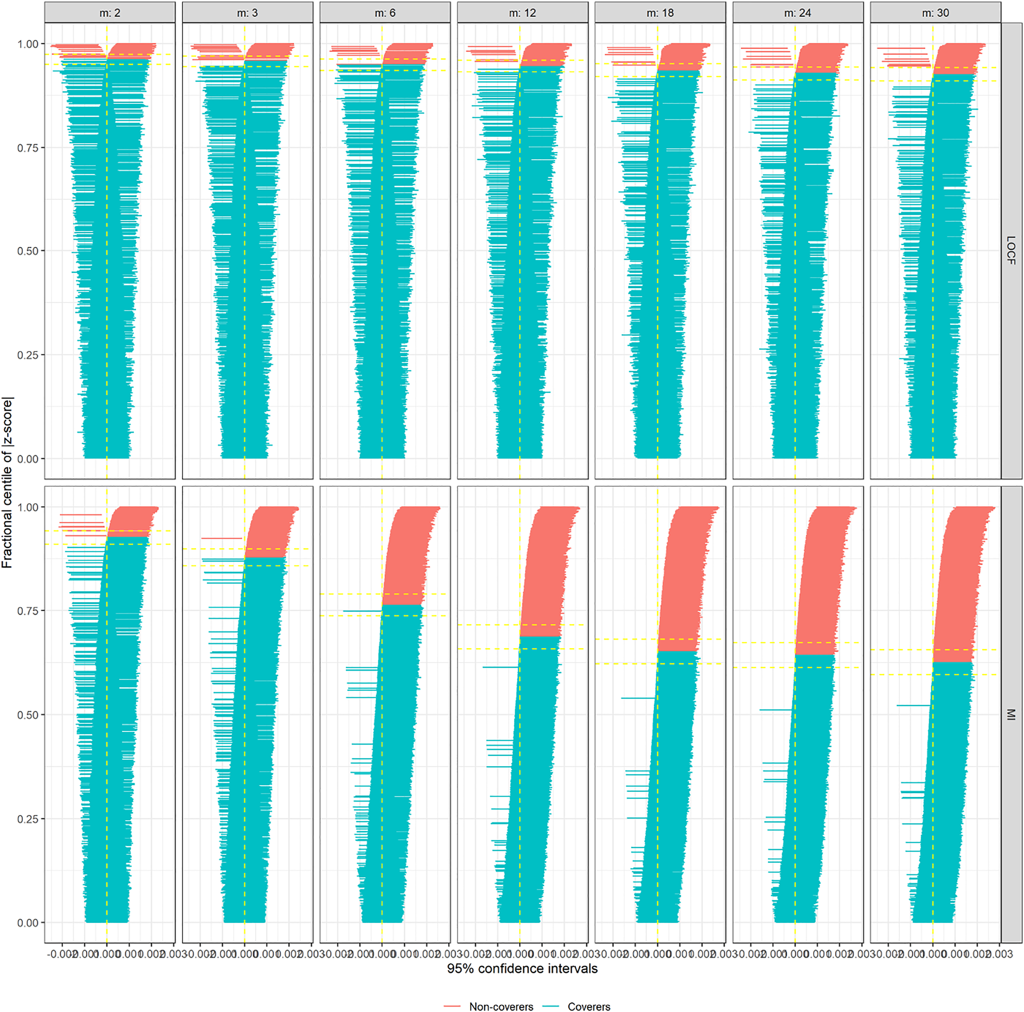

When trial size varies

We consider scenario 3 as our base scenario where σ = 2. Zip plot is shown in Supplementary Figures A9. As the sample size increases, usually, the undercoverage problem becomes more prominent if this issues is due to bias ²¹. From scenarios 4 (n = 2, 000) and 5 (n = 250), we can see confirmation that undercoverage is being driven by bias when sample size increases (Supplementary Figures A10 and A11, respectively).

Choice of multiple imputation methods

Indeed multiple imputation could use many different imputation models, such as predictive mean matching, 2-level predictive mean matching, random forest, Bayesian linear regression and linear regression. We used all of these different imputation models for scenario 3 (σ = 2). When the imputation models were built using Bayesian linear regression and linear regression, they looked very similar to the one built using predictive mean matching, in terms of MSE (See Supplementary Figures A12 and A14). For more complicated methods such as 2-level predictive mean matching and random forest, MSEs are very similar, but had a slightly higher trend (Supplementary Figures A13).

Choice of the effect estimate

We used target effect estimates in both RD and OR in scenario 3. The statistical properties remained the same regardless of the choice of effect estimate. The zip plots are shown in Supplementary Figures A9 and A15.

When all confounders are measured and adjusted

When confounder U is measured and adjusted in scenario 3, the issue with bias and undercoverage are nearly eliminated for both LOCF and MI methods (Supplementary Figure A16). The same is true when U is not a confounder, but merely a risk factor for the outcome (scenario 6; Supplementary Figure 17).

Case study

Study setting

The Lipid Research Clinics Coronary Primary Prevention Trial was a double-blinded, multicenter randomized controlled trial conducted. The aim that we consider is to estimate the effect of cholestyramine treatment on the risk of coronary heart disease death or non-fatal myocardial infarction, after adjusting for non-adherence. After screening, 3, 550 male subjects aged 35–59 years were eligible to randomize to treatment with cholestyramine or a placebo. After randomization, the first two visits occurred at 2 weeks intervals, and all successive visits occurred at 2 months intervals. According to the protocol, there were 32 time-varying covariates with different measurement frequencies; at each visit, each third visit, and each sixth visit. Approximately 80% of participants became non-adherent by the end of their follow-up. About 7% of participants experienced the event of interest. The details of the study, covariates, adherence, and the outcome can be found elsewhere^9–11,35. The covariates names and necessary IPAW modelling detailed are reported in Supplementary section 3. There existed notable variabilities in some post-randomization prognostic factors in the standard deviation (SD) scale. Half of the SDs associated with continuous factors were less than 2, and the rest were greater or equal to 2.

Estimating effects under two imputation methods

Similar to the simulations, multiple imputation used 10 imputations utilizing predictive mean matching, and all available covariates, outcome and the Nelson–Aalen estimate were used in building the imputation model. In Table 2, we reported the log-HR, robust SE, OR, and 95% CI from the IPAW estimators under consideration. We observed that the IPAW estimates with the LOCF versus multiple imputation are approximately identical.

Table 2.

The effect of cholestyramine treatment on the risk of coronary heart disease death or non-fatal myocardial infarction, after adjusting for non-adherence, estimated using the inverse probability of adherence weighted per-protocol effect measures with irregular measurement frequencies of time-varying covariates from the Lipid Research Clinics Coronary Primary Prevention Trial¹.

IPAW estimator^1,2	Weights		log-HR		HR
	Mean	Min-max	Estimate	SE.	Estimate	95% CI
LOCF	1.03	0.15–11.00	-0.24	0.291	0.79	0.44–1.39
MI	1.03	0.14–9.99	-0.25	0.291	0.78	0.44–1.38

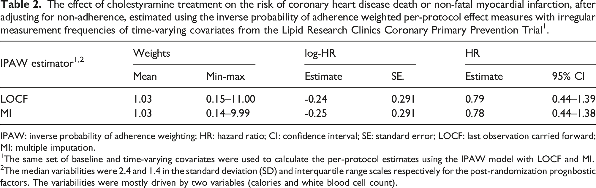
IPAW: inverse probability of adherence weighting; HR: hazard ratio; CI: confidence interval; SE: standard error; LOCF: last observation carried forward; MI: multiple imputation.

¹The same set of baseline and time-varying covariates were used to calculate the per-protocol estimates using the IPAW model with LOCF and MI.

²The median variabilities were 2.4 and 1.4 in the standard deviation (SD) and interquartile range scales respectively for the post-randomization prognbostic factors. The variabilities were mostly driven by two variables (calories and white blood cell count).

Discussion

Summary

For pragmatic trials, not addressing incomplete adherence can lead to biased treatment effect estimate. Sophisticated statistical methods such as IPAW estimators are gaining more recognition and popularity in the per-protocol analyses due to their ability to address ²⁰. Tutorials, editorials, and guideline documents are being written to raise awareness, and to fill the gap in the renewed interest about this method in recent years.^1,2,22 The strength of this method lies in utilizing high-quality pre and post-randomization factors in the analysis that can predict the adherence pattern, and appropriately adjusting those factors in the analysis via inverse probability weighting. However, infrequent measurement of the post-randomization factors can threaten the validity of this method.⁴ Due to cost and logistical constraints, more frequent in-person measurements of necessary factors (e.g., laboratory testing) may not always be possible to schedule in the trial design, leading to possible gaps in the longitudinal measurements of post-randomization factors, resulting in sub-optimal IPAW estimates.

For estimation of per-protocol effect using the IPAW model, we organize the data in a long-format, where we record data about pre-randomization factors, as well as observations of each time-varying variables, such as changes in treatment and post-randomization factors by time index (e.g., could be in months).²² Under MCAR assumption, we have considered two imputation methods, LOCF and multiple imputation, to impute values for the months where measurements of any post-randomization factor were not recorded. In the following comparisons, zip plots have provided visual illustrations of the overall performances of the imputation methods in most scenarios. We have also used other performance measures, such as bias, precision measures and coverage, to investigate further details about the reasoning behind the poor performances in some of the zip plots.

Based on our simulation, here is the summary of our findings: (1) when there does not exist any confounding, the statistical properties of IPAW estimates from either imputation method are desirable and similar in terms of reduced bias, similar precision levels, and achieved nearly nominal coverage. (2) Same is true when there exists confounding, and all of the necessary confounders and measured and adjusted. (3) However, bias levels from both approaches increase with the increment of the gap in measurement frequency, when there exists an unmeasured baseline confounder, that leads to treatment-condfounder feedback²². Interestingly, the model SEs and empirical SEs from both LOCF and multiple imputation approaches were comparable, bias from multiple imputation approach was slightly elevated compared to that from the LOCF approach. This phenomenon resulted in LOCF having better coverage probabilities compared to that of multiple imputation, particularly when the variance of the post-randomization confounder (that was imputed) was low. (4) When the variance of the post-randomization confounder was slightly higher, bias levels, coverage probabilities as well as zip plots from LOCF did not have any notable advantages in terms of statistical performances compared to those from multiple imputation. This observation is intuitive, that LOCF would perform better for imputations of a post-randomization prognostic factor when there is less variability in the post-randomization prognostic factor (or when they remain constant over time), and the imputed values would likely be close enough to true unmeasured value. However, such an advantage would diminish as soon as the variability in the post-randomization prognostic factor increases. (5) For even larger variance of the post-randomization confounder, some model SE from LOCF is associated with higher variability, and the coverage probabilities decrease further. (6) When the trial size was increased, the coverage probabilities were drastically reduced. This observation is also intuitive that, with a larger sample size, the bias would be more emphasized, resulting in deteriorating coverage. (7) We have primarily used predictive mean matching to impute observations in the multiple imputation approach. Given that there exist many multiple imputation methods, we also used a number of other imputation methods within the multiple imputation approach. The results were generally the same. (8) We are estimated OR instead of RD, and the statistical performances from the simulation remained the same.

Contextualizing the current findings in the literature

For marginal structural models (e.g., as-treated analyses), a simulation study suggested that a large variance of the time-dependent confounder was associated with poor performance of the multiple imputation approach.³⁶ For our per-protocol setting, performance of both LOCF and multiple imputation apparently deteriorated in terms of coverage probabilities when a large variance of the post-randomization prognostic factor was considered. Hughes et al.³⁷ argued that choice of imputation method should be dictated by proportion, pattern, and reasons of missingness (or non-adherence in our example), and that even complete case analysis may be more suitable than multiple imputation in some settings.

Impact of using different imputation methods in the case study

Using LOCF imputation method for imputation, a previous study observed a 26% reduction in risk (although insignificant) using the IPAW estimator.¹¹ However, out of 38 time-varying covariates used in that study, six of them were associated with high percentages of missing values (e.g., data was not collected for these six covariates according to the protocol). However, our study aims to understand the impact of imputation methods for the values that were unobserved due to protocol (e.g., specified gaps in the measurement schedule, and hence likely MCAR). Hence, in this study, we restricted the analysis to 32 time-varying covariates measured relatively completely at each visit, each third visit, or each sixth visit according to the protocol. In our study, when we used LOCF for imputing the measurements in the scheduled gaps, there was a 21% reduction in risk (insignificant) of coronary heart disease death or non-fatal myocardial infarction in the cholestyramine treatment group than placebo. When we used multiple imputation, we found a 22% reduction in risk (again insignificant). Based on our simulation results, we know variance of the post-randomization prognostic factor is an important deciding factor of the imputation method. Given that we observe notable variabilities in about half of the post-randomization prognostic factors, we would prefer the results from the multiple imputation approach.

Strengths, limitations, and future directions

Researchers often focus primarily on the bias as a measure of performance for a statistical approach.³⁸ However, precision estimates and whether estimates are subject to undercoverage are also essential considerations for an estimator, particularly for inverse probability weighted estimates, for which there exists a bias-variance trade-off. Zip plots are important instruments in assessing the performances of different estimators. In the current work, they were used to compare the performances of LOCF and multiple imputation in estimating per-protocol effect from IPAW model.

In the LOCF approach, unavailable values are being imputed by the last measured value of the same post-randomization prognostic factor, and some imprecise measurement, as well as residual confounding, is expected.⁴ Alternatively, for multiple imputation approach is utilizing an imputation model, that includes other covariates, outcome event and Nelson–Aalen estimate of cumulative hazard to predict the values of the post-randomization prognostic factor. One could argue that the use of potential future information may be inducing reverse causation in the process, whereas LOCF is free from such criticism.²⁰

The simulation setting we considered was focused on answering a very specific question of which imputation method help impute better values under MCAR. That is why we resorted to having infrequent measurements for only one post-randomization prognostic factor. However, it is possible to extend the simulation setting to more complicated scenarios, dealing with infrequent measurements of multiple post-randomization prognostic factors, as well as treatment status.¹⁶ To keep the message simple, we did not consider loss to follow-up in the simulation similar to previous simulations.^4,16

Our simulation settings only considered a null treatment effect (OR = 1, or RD = 0), as was proposed in Young et al.⁴ Mosquera¹⁶ previously extended the algorithm of Young et al.⁴ to accommodate non-null treatment effects. They have estimated per-protocol treatment effects via the same IPAW estimator we have used after imputing the unobserved values via LOCF to handle the sparse measurements. When magnitudes of the true treatment effect were varied (between log-OR -1.5 to 1.5, including 0 as a null value) in their simulations, after holding all other parameters constant, the corresponding per-protocol effect estimates obtained from those simulations remained unbiased. Assessing results from that simulation study, we have no reason to believe that a non-null treatment effect would have impacted the findings or conclusions from our simulation.

One advantage of multiple imputation that we did not consider in our simulations, is the ability to incorporate auxiliary information in the imputation model. Auxiliary variables are those that are either associated with partially measured factors, some proxy information of the variable needing imputation or the reasons of missingness³⁷. Utilizing such auxiliary information, the performance of multiple imputation can be potentially enhanced in future simulations. In our analysis, we have used Rubin’s variance estimator, which can produce conservative or anti-conservative confidence intervals in various setting. Future research can consider alternative approaches.^39,40

MCAR is a strong, and often unrealistic assumption under real-world considerations. The possibility of MCAR in routinely collected data from laboratories or clinics is not unrealistic, but such assumption can not be confirmed or tested from the dataset. Experts should be consulted to assess the plausibility of such an assumption.⁶

Regulatory agencies, such as U.S. Food and Drug Administration, emphasize primary clinical efficacy evidence obtained from intent-to-treat analyses instead of per-protocol for drug approval. In the current work, however, we have not considered intention-to-treat analyses, as our focus is about pragmatic trials, not clinical trials. While randomized clinical trials are designed to seek regulatory approval for drugs, pragmatic trials are designed to guide patients, clinicians and caregivers to make decisions about patient’s treatment choices, and hence can help answering patient-oriented real-world questions². Numerous previous analyses and simulations focusing on pragmatic trials have repeatedly shown that when trials are subject to incomplete adherence (usually the case for pragmatic trials), effect estimates obtained from per-protocol analyses are superior to those obtained from intention-to-treat analyses under a variety of treatment effect estimation situations in properly accounting for incomplete adherence.^{4,16,18,20,22,41} Hence, we have decided not to re-examine this comparison in the current work.

Conclusion

We were particularly interested in the infrequent measurement (e.g., after certain months) of a post-randomization prognostic factor by design, in the presence of incomplete adherence. Through our simulation, we found that variance of the post-randomization prognostic factor can be an important indicator for choosing a suitable imputation method for that factor. For higher variability of the post-randomization prognostic factor, multiple imputation approach shows desirable statistical properties under MCAR assumption; otherwise LOCF approach can be adequate. Different choices of imputation methods (e.g., predictive mean matching or otherwise) within multiple imputation approach did not impact the result noticeably. Both LOCF and multiple imputation methods performed well in terms of zip plot or statistical properties under consideration, when there is no confounding or when all necessary confounders are adjusted.

Supplemental material

Supplemental material - Considerations for choosing an imputation method for addressing sparse measurement issues dictated by the study design - An illustration from per-protocol analysis in pragmatic trials for Research Methods in Medicine & Health Sciences

Supplementary material for Considerations for choosing an imputation method for addressing sparse measurement issues dictated by the study design - An illustration from per-protocol analysis in pragmatic trials by Mohammad Ehsanul Karim and Md Belal Hossain in Research Methods in Medicine & Health Sciences.

Footnotes

Declaration of conflicting interests

The author(s) declared no potential conflicts of interest with respect to the research, authorship, and/or publication of this article.

Funding

The author(s) disclosed receipt of the following financial support for the research, authorship, and/or publication of this article: This study is supported by BC Support Unit and Natural Sciences and Engineering Research Council of Canada.

Data availability statement

The software code used for analysis is available in GitHub: . The trial dataset access can be requested from National Heart, Blood, and Lung Institute. The analysis of secondary and de-identified data was exempt from the requirements for research ethics approval both in accordance with the University of British Columbia Policy 89 and in accordance with the provisions of the Tri-Council Policy Statement: Ethical Conduct for Research involving Humans, Article 2.5.

ORCID iDs

Mohammad Ehsanul Karim

Md Belal Hossain

Supplemental material

Supplemental material for this article is available online.

References

Hernán

Robins

. Per-protocol analyses of pragmatic trials. N Engl J Med 2017; 377(14): 1391–1398.

Murray

Swanson

Hernán

. Guidelines for Estimating Causal Effects in Pragmatic Randomized Trials, Methodology, 2019.

Robins

Finkelstein

. Correcting for noncompliance and dependent censoring in an aids clinical trial with inverse probability of censoring weighted (ipcw) log-rank tests. Biometrics 2000; 56(3): 779–788.

Young

Vatsa

Murray

, et al. Interval-cohort designs and bias in the estimation of per-protocol effects: a simulation study. Trials 2019; 20(1): 1–9.

Jakobsen

JC.

Gluud

Wetterslev

, et al. When and how should multiple imputation be used for handling missing data in randomised clinical trials–a practical guide with flowcharts. BMC Medical Research Methodology 2017; 17(162): 1–10, DOI: 10.1186/s12874-017-0442-1

Leyrat

Carpenter

Bailly

, et al. Common methods for handling missing data in marginal structural models: what works and why. Am Journal Epidemiology 2021; 190(4): 663–672.

Liu

S-H.

Chrysanthopoulou

Chang

, et al. Missing data in marginal structural models: a plasmode simulation study comparing multiple imputation and inverse probability weighting. Med Care 2019; 57(3): 237–243.

Moodie

Delaney

Lefebvre

, et al. Missing confounding data in marginal structural models: a comparison of inverse probability weighting and multiple imputation. The International Journal Biostatistics 2008; 4(1): Article–13.

The Lipid Research Clinics Program . The coronary primary prevention trial: design and implementation. J Chronic Dis 1979; 32(9–10): 609–631.

10.

Wanis

Madenci

Hernán

, et al. Adjusting for adherence in randomized trials when adherence is measured as a continuous variable: an application to the lipid research clinics coronary primary prevention trial. Clin Trials 2020; 17(5): 570–575.

11.

Mosquera

Karim

Hossain

. Properties of inverse probability of adherence weighted estimator of the per-protocol effect for sustained treatment strategies under different data generating mechanisms and adherence patterns. Under review, 2022.

12.

Carpenter

Kenward

. Missing Data in Randomised Controlled Trials: a Practical Guide, London, UK: LSHTM. 2007.

13.

Molenberghs

Thijs

Jansen

, et al. Analyzing incomplete longitudinal clinical trial data. Biostatistics 2004; 5(3): 445–464.

14.

Yang

Eaton

, et al. Application of marginal structural models in pharmacoepidemiologic studies: a systematic review. Pharmacoepidemiol Drug Safety 2014; 23(6): 560–571.

15.

Mojaverian

Moodie

Bliu

, et al. The impact of sparse follow-up on marginal structural models for time-to-event data. Am Journal Epidemiology 2015; 182(12): 1047–1055.

16.

Mosquera

. Exploring Inverse Probability Weighted Per-Protocol Estimates to adjust for Non-adherence Using Post-randomization Covariates: a Simulation Study. Master’s thesis, University of British Columbia, 2020.

17.

Cho

Keithly

Kurgansky

, et al. Early convalescent plasma therapy and mortality among us veterans hospitalized with non-severe covid-19: an observational analysis emulating a target trial. The J Infect Dis 2021.

18.

Murray

Caniglia

Swanson

, et al. Patients and investigators prefer measures of absolute risk in subgroups for pragmatic randomized trials. J Clinical Epidemiology 2018; 103: 10–21.

19.

Kaufman-Janette

Taylor

Cox

, et al. Efficacy and safety of a new resilient hyaluronic acid dermal filler, in the correction of moderate-to-severe nasolabial folds: a 64-week, prospective, multicenter, controlled, randomized, double-blind and within-subject study. J Cosmetic Dermatology 2019; 18(5): 1244–1253.

20.

Murray

Claggett

Granger

, et al. Adherence-adjustment in placebo-controlled randomized trials: an application to the candesartan in heart failure randomized trial. Contemp Clinical Trials 2020; 90: 105937.

21.

Morris

White

Crowther

. Using simulation studies to evaluate statistical methods. Stat Medicine 2019; 38(11): 2074–2102.

22.

Murray

Caniglia

Petito

. Causal survival analysis: a guide to estimating intention-to-treat and per-protocol effects from randomized clinical trials with non-adherence. Res Methods Med Health Sci 2021; 2(1): 39–49.

23.

D’Agostino

Lee

M-L

Belanger

, et al. Relation of pooled logistic regression to time dependent cox regression analysis: the framingham heart study. Stat Medicine 1990; 9(12): 1501–1515.

24.

Ngwa

Cabral

Cheng

, et al. A comparison of time dependent cox regression, pooled logistic regression and cross sectional pooling with simulations and an application to the framingham heart study. BMC Medical Research Methodology 2016; 16(148): 1–12, DOI: 10.1186/s12874-016-0248-6

25.

Naimi

Whitcomb

. Estimating risk ratios and risk differences using regression. Am J Epidemiol 2020; 189(6): 508–510.

26.

Schafer

. Longitudinal data failure. In: Van Buuren

(ed). Flexible Imputation of Missing Data. CRC Press; 2018, pp. 311–336. chapter 11.

27.

White

Royston

. Imputing missing covariate values for the cox model. Stat Medicine 2009; 28(15): 1982–1998.

28.

Rubin

. Multiple Imputation for Nonresponse in Surveys, 81. New Jersey, USA: John Wiley & Sons, 2004.

29.

Rubin

. Multilevel multiple imputation. In: Van Buuren

(ed). Flexible Imputation of Missing Data. Florida, USA: CRC Press; 2018, pp. 29–62. chapter 2.

30.

Enders

. Multilevel multiple imputation. In: Van Buuren

(ed). Flexible Imputation of Missing Data. Florida, USA: CRC Press; 2018, pp. 197–240. chapter 7.

31.

Shah

Bartlett

Carpenter

, et al. Comparison of random forest and parametric imputation models for imputing missing data using mice: a caliber study. Am Journal Epidemiology 2014; 179(6): 764–774.

32.

Burton

Altman

Royston

, et al. The design of simulation studies in medical statistics. Stat Medicine 2006; 25(24): 4279–4292.

33.

Wicklin

. A Zipper Plot for Visualizing Coverage Probability in Simulation Studies, New Jersey, USA: John Wiley & Sons. 2018.

34.

Gasparini

. rsimsum: Summarise results from monte carlo simulation studies. J Open Source Softw 2018; 3: 739. DOI: 10.21105/joss.00739

35.

The Lipid Research Clinics Program . The lipid research clinics coronary primary prevention trial results. i. reduction in incidence of coronary heart disease. The J Am Med Assoc 1984; 251: 351–364.

36.

Vourli

Touloumi

. Performance of the marginal structural models under various scenarios of incomplete marker’s values: a simulation study. Biometrical J 2015; 57(2): 254–270.

37.

Hughes

Heron

Sterne

, et al. Accounting for missing data in statistical analyses: multiple imputation is not always the answer. Int Journal Epidemiology 2019; 48(4): 1294–1304.

38.

Little

Rubin

. Statistical analysis with Missing Data, 793. New Jersey, USA: John Wiley & Sons, 2019.

39.

Robins

Wang

. Inference for imputation estimators. Biometrika 2000; 87(1): 113–124.

40.

Hughes

Sterne

Tilling

. Comparison of imputation variance estimators. Stat Methods Medical Research 2016; 25(6): 2541–2557.

41.

Murray

Hernán

. Improved adherence adjustment in the coronary drug project. Trials 2018; 19(1): 1–4.

Supplementary Material

Please find the following supplemental material available below.

For Open Access articles published under a Creative Commons License, all supplemental material carries the same license as the article it is associated with.

For non-Open Access articles published, all supplemental material carries a non-exclusive license, and permission requests for re-use of supplemental material or any part of supplemental material shall be sent directly to the copyright owner as specified in the copyright notice associated with the article.

0.00 MB

1.63 MB