Sage Journals: Discover world-class research

Abstract

Background

Follow-up frequency is an important design parameter in longitudinal studies. We quantified the impact of reducing follow-up frequency on the precision of estimated regression parameters, and investigated the impact of incorrectly assuming an exchangeable correlation structure on estimates of the loss of precision resulting from reduced follow-up.

Methods

We estimated the loss in precision on deleting every second observation from three longitudinal cohorts: patients with Childhood Systemic Lupus Erythematosus (cSLE), the Canadian Haemophilia Prophylaxis Study (CHPS), and patients with Juvenile Dermatomyositis (JDM). We compared these results with those from a theoretical formula assuming an exchangeable correlation structure.

Results

The increase in sample size needed to compensate for halving follow-up frequency was 9%, 6% and 28% for the cSLE, CHPS and JDM cohorts respectively. Under the assumption of an exchangeable correlation, the estimated increases in sample size were 22%, 11% and 10% respectively.

Conclusions

Reducing follow-up frequency can result in minimal loss of information, as seen in the CHPS cohort. While using a theoretical formula based on an exchangeable correlation structure is convenient, it can be inaccurate when the true correlation structure is not exchangeable.

Keywords

Sample size longitudinal data correlation power

Background

Investigators planning longitudinal studies must strike a balance between obtaining rich information from each subject through frequent follow-up, and maintaining a reasonable burden of participation for both patient and physician. This is of particular concern in studies of rare diseases, where the total number of respondents is limited and thus the risk of a patient or their physician declining to participate due to intensive follow-up must be carefully weighed against maximizing the information available for each patient. A number of authors have noted the increase in precision upon collecting more frequent follow-up from each participant.^1–4 We approach the question from the opposite direction, asking whether in a future study we should follow up as often as we have done in the past.

The frequency of follow-up and the number of patients recruited are design parameters that must be considered in tandem. To help determine a suitable frequency of follow-up, methods for power-based sample size calculations can be helpful. Kirby et al.⁵ provide sample size formulae for a randomized controlled trial with a longitudinally assessed outcome, under the assumption of a damped exponential correlation structure.⁶ Overall⁷ considers an exponential correlation structure and the case where treatment effects can vary over time. Liu and Liang present a formula for sample size calculations with a GEE⁸ under a general correlation structure with time-invariant discrete covariates, while Liu et al.⁹ extended this to an additional level of clustering and Jung¹⁰ extend to include comparison of slopes in the presence of missing data. Sample size calculations thus require information on both the correlation structure of longitudinal observations within patients, and the values of the parameters of the chosen structure.

Liu and Liang⁸ note that their sample size formula simplifies considerably when the correlation structure is exchangeable (i.e., the correlation between any two observations from the same individual is the same, no matter how far apart the observations are in time) and the covariates are time-invariant. In this case the formula is just the usual formula for uncorrelated data, multiplied by the design effect.¹¹ The design effect was first introduced in 1965¹¹ and became well known in the context of cluster-randomized trials.^12,13 Since it depends on just two parameters (the number of observations per cluster and the correlation between any pair of observations from the same cluster), it is much easier to use than the general formula. It may thus be appealing to investigators planning longitudinal studies to assume an exchangeable correlation structure, even if this is not in fact plausible. Thus, it would be helpful to understand the impact of this simplifying assumption in practice.

The objective of this paper is twofold. Firstly, we use three studies in paediatric rheumatology^14–16 to investigate empirically the loss of information resulting from less frequent follow-up. Secondly, by comparing the empirical loss of information to the loss of information calculated using a theoretical formula based on the design effect, we investigate the impact of using this simplified formula when the underlying assumptions are not met.

Methods

Sample size inflation factor (SSIF)

The loss of information on reducing the frequency of follow-up can be quantified in terms of the inflation in sample size that would be required in order to maintain the same level of precision as is to be had by using all the observations from each patient.

Suppose we have N observations from n patients, and that the variance of the regression coefficient of interest is v on using the full dataset. Further, suppose that deleting 100x% of the observations from each patient causes the variance of the regression coefficient to increase by 100 y% to (1 + y)v. Since variance is proportional to the inverse of the sample size, if we were to use a sample size n* = n(1 + y) with the reduced frequency of observation, we would recover the original variance v. That is, inflating the sample size by 100 y% recovers the original level of precision. We call y the sample size inflation factor (SSIF). Under the assumptions of an exchangeable correlation structure (with correlation ρ), that each patient has m measurements, and that all the covariates in the regression model are time-invariant, the SSIF has a simple closed-form expression

SSIF = \frac{1 + (m (1 - x) - 1) ρ}{(1 + (m - 1) ρ) (1 - x)}

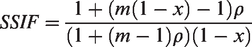
A derivation of this result is available in the online Appendix.

Statistical methods

For each of the three datasets, analysis began by describing the correlation structure. The regression model of interest was fit using ordinary least squares omitting each subject in turn, and the jackknife residuals calculated by taking the difference between the observed values for the omitted subject and the predicted values from the model omitting that subject’s data. These jackknife residuals were standardized to have unit variance by deriving a smooth loess fit of the square residuals as a function of time and dividing the residuals by the square root of the fitted values. Within each subject, all possible pairs of observations from the same subject at different times were identified, and their cross-products calculated along with the lag between the observations. The correlation between standardized jackknife residuals from the same subject as a function of the lag was estimated through a smooth fit of the cross-products as a function of the lags, derived using the loess function in R.¹⁷

Using the full dataset and an exchangeable working correlation structure, a GEE was fitted to compute the mean correlation ρ between any two observations from the same individual. This was used to compute the theoretical SSIF for each dataset for x = 1/2, 2/3, 3/4, 4/5, and 5/6 (i.e. retaining every second, every third, every fourth, and every fifth observation).

We compared this to the empirical SSIF by randomly retaining every second, every third, every fourth and every fifth observation. Specifically, if retaining every jth observation, for each subject we randomly selected one of the first j observations to be the first observation to be retained, then retained every jth observation thereafter. For each value of x, this procedure was repeated 1000 times. The regression model was run on each of the resulting datasets using a GEE with an independent working correlation structure, and the standard error of the regression coefficient was noted. These standard errors were compared to the standard error using all the data, and the SSIF for each dataset calculated as the square of the ratio of the standard errors. The SSIFs were summarized using the mean and standard deviation (SD). A flow chart of the analytic steps is given in the online Appendix.

Data

We considered three studies in paediatric rheumatology, described below and summarized in Table 1.

Table 1.

Characteristics of the three cohorts.

	cSLE	CHPS	JDM
Sample size	473	56	95
Median (IQR) number of measurements per patient	18 (11–27)	22 (17–30)	13 (9–15)
Median (IQR) follow-up (years)	3.6 (2.0–5.4)	9.3 (7.9–14.0)	3.5 (2.4–3.8)
Longitudinally measured outcome	Systemic Lupus Erythematosus Disease Activity Index 2000	Number of bleeds (log transformed)	Disease activity Score
Covariate in model	Prednisone dose 3 months prior	Age at first joint bleed	Cutaneous nailfold changes

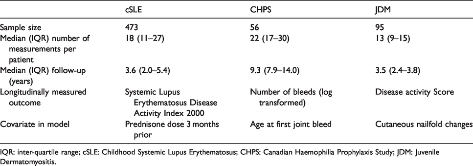
IQR: inter-quartile range; cSLE: Childhood Systemic Lupus Erythematosus; CHPS: Canadian Haemophilia Prophylaxis Study; JDM: Juvenile Dermatomyositis.

Childhood onset Systemic Lupus Erythematosus (cSLE)

In order to describe the longitudinal trajectory of patients with Childhood onset Systemic Lupus Erythematosus (cSLE) and to identify predictors of damage, 473 patients initially treated at The Hospital for Sick Children were followed from the time of diagnosis into adulthood. In this analysis, the median number of visits per patient was 18 (inter-quartile range (IQR) 11–27).

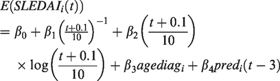
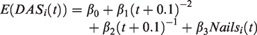
For the purposes of this study, we consider the relationship between prednisone dose in the previous quarter on disease activity, measured through the Systemic Lupus Erythematosus Disease Activity Index 2000 (SLEDAI),¹⁸ adjusting for age at diagnosis and time since diagnosis. Specifically, the regression model considered is

\begin{array}{l} E (SLEDA I_{i} (t)) \\ = β_{0} + β_{1} {(\frac{t + 0.1}{10})}^{- 1} + β_{2} (\frac{t + 0.1}{10}) \\ \times \log (\frac{t + 0.1}{10}) + β_{3} a gedia g_{i} + β_{4} p r e d_{i} (t - 3) \end{array}

where SLEDAI_i(t) is the SLEDAI score for subject i at month t, agediag_i is subject i's age at diagnosis, and pred_i(t-3) is the time-varying prednisone dose (in mg) for subject i three months before time t.

The Canadian Haemophilia Prophylaxis Study (CHPS)

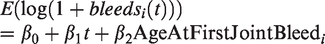
The Canadian Hemophilia Prophylaxis Study recruited 56 boys with severe hemophilia A.¹⁴ The protocol required that subjects report the number of bleeds in the current month, every three months during the first five years of the study, then every half a year subsequently. The median number of records per patient was 22 (IQR 17–30).

For the purposes of this study, we regressed the number of bleeds in a given month (log-transforming to remove skewness) onto age at first joint bleed and time since recruitment. The parameter of interest was the regression coefficient of age at first joint bleed. Six joints were considered: left ankle, right ankle, left knee, right knee, left elbow, and right elbow. Results were similar across joints and we present the results for the left ankle only. The regression model was

\begin{array}{l} E (\log (1 + bleed s_{i} (t))) \\ = β_{0} + β_{1} t + β_{2} {AgeAtFirstJointBleed}_{i} \end{array}

Juvenile dermatomyositis (JDM)

Since 1991, children presenting in a clinic treating juvenile dermatomyositis have been enrolled at diagnosis into a research cohort.¹⁶ At the time of creating this dataset, 95 children had been recruited. In the analysis considered here, follow-up was capped at 4 years to avoid the possibility of informative censoring due to transitions to adult care around age 18. There was a median of 13 visits per patient (IQR 10–16).

For the purposes of this study, the association of interest is the relationship between the presence of cutaneous nailfold changes on the DAS at the next visit. Disease activity was measured using a modified disease activity score (DAS) capturing the musculoskeletal and cutaneous manifestations of JDM,¹⁹ with higher scores indicating worse disease activity. Specifically, the model considered was

\begin{array}{l} E (D A S_{i} (t)) = β_{0} + β_{1} (t + 0.1)^{- 2} \\ + β_{2} (t + 0.1)^{- 1} + β_{3} N ail s_{i} (t) \end{array}

where t is time in years and Nails_i(t)=1 if patient i had cutaneous nailfold changes at the last visit and zero otherwise.

Results

Figure 1 shows the correlation between observations from the same subject as a function of the time between measurements for each of the three datasets. For each dataset, the correlation decreases as the time between measurements increases, indicating that the correlation structure is not exchangeable and an exponential, Gaussian or other spatial correlation structure would be more appropriate. More information on the correlation structures is available in the online Appendix.

Figure 1.

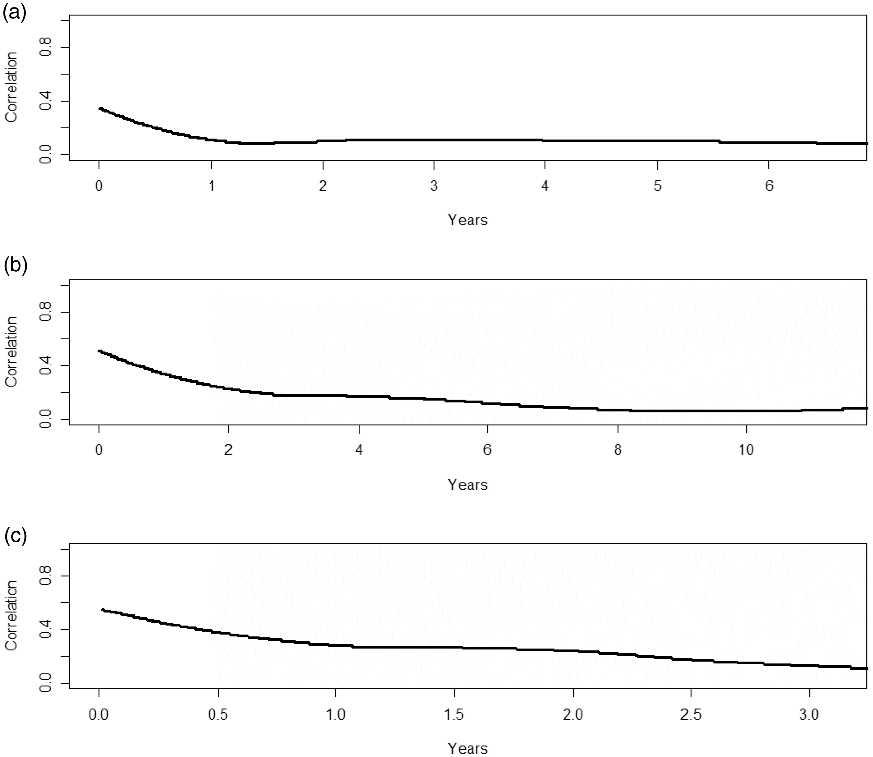
Autocorrelation plots for (a) the Childhood Systemic Lupus Erythematosus (cSLE) study, (b) the Canadian Haemophilia Prophylaxis Study (CHPS), and (c) the Juvenile Dermatomyositis (JDM) study.

The estimated ICCs under working exchangeability were 0.211 for the cSLE dataset, 0.259 for the CHPS dataset, and 0.413 for the JDM dataset.

Table 2 shows the inflation in standard errors when the observation frequency is diminished, expressed both in terms of the observed standard errors and the SSIF. For the CHPS dataset, the frequency of observation could be halved and require only a 6% increase in sample size to compensate for the resulting loss of information. Similarly, for a three-fold reduction in measurement frequency, a 9% increase in sample size would be needed. The other datasets showed a greater loss of information, with the cSLE dataset requiring a 9% increase in sample size on halving the visit frequency, and the JDM dataset requiring a 28% increase in sample size.

Table 2.

Impact of reducing the observation frequency in each of the three cohorts, illustrated in terms of the standard error of the regression coefficient of interest (expressed s the mean over 1000 randomly generated datasets), and the sample size inflation factor, the latter being estimated both empirically and theoretically.

Cohort		Retaining every
Cohort		2nd	3rd	4th	5th	6th
	Full dataset	Standard Error of regression coefficient
cSLE	0.0282	0.0293	0.0308	0.0321	0.0341	0.0353
CHPS	0.0637	0.0655	0.0663	0.0685	0.0694	0.0712
JDM	0.188	0.213	0.244	0.267	0.285	0.305
		Sample size inflation factors presented as mean (standard deviation) for empirical estimates
cSLE	Empirical	1.09 (0.13)	1.20 (0.14)	1.30 (0.18)	1.47 (0.20)	1.59 (0.30)
	Theoretical	1.22	1.44	1.67	1.89	2.11
CHPS	Empirical	1.06 (0.15)	1.09 (0.17)	1.16 (0.21)	1.20 (0.24)	1.26 (0.28)
	Theoretical	1.11	1.22	1.33	1.44	1.55
JDM	Empirical	1.28 (0.13)	1.69 (0.22)	2.02 (0.28)	2.31 (0.34)	2.85 (0.43)
	Theoretical	1.10	1.20	1.30	1.40	1.51

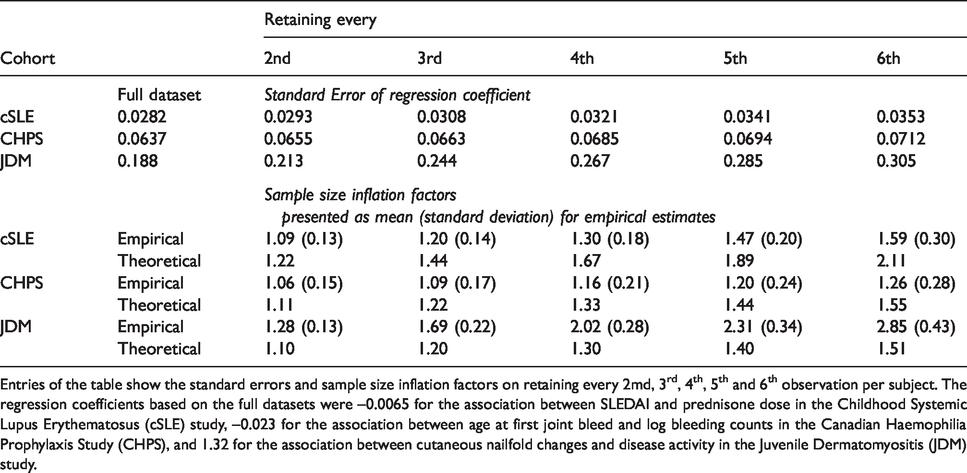
Entries of the table show the standard errors and sample size inflation factors on retaining every 2md, 3^rd, 4^th, 5^th and 6^th observation per subject. The regression coefficients based on the full datasets were –0.0065 for the association between SLEDAI and prednisone dose in the Childhood Systemic Lupus Erythematosus (cSLE) study, –0.023 for the association between age at first joint bleed and log bleeding counts in the Canadian Haemophilia Prophylaxis Study (CHPS), and 1.32 for the association between cutaneous nailfold changes and disease activity in the Juvenile Dermatomyositis (JDM) study.

Turning to more drastic reductions in observation frequency, for the CHPS dataset, a six-fold reduction required a 26% increase in sample size. The other datasets required greater increases: 59% for the cSLE dataset and 185% for the JDM dataset.

There was variation in the empirical SSIFs, as evidenced by their standard errors (Table 2). The corresponding inter-quartile ranges for the empirical SSIFs on omitting every second observation were (0.96, 1.20) for the cSLE dataset, (0.95, 1.16) for the CHPS dataset, and (1.02, 1.32).

The theoretical estimates of the sample size inflation factors differed from the empirical estimates; for the lupus and CHPS cohorts the theoretical estimates were overestimates, whereas for the JDM cohort the theoretical estimates were underestimates.

Discussion

Our results show that in two of the three studies, follow-up could have been half as often with a minimal loss of information, requiring on average less than a 10% inflation in sample size to compensate for the loss of information. The magnitude of the difference between the empirical and theoretical estimates of the SSIF was large enough that it could lead to a different decision. For example, in the lupus dataset a halving of observation frequency required just a 9% increase in sample size, however the theoretical estimate suggested that a 22% increase in sample size would be needed.

That the theoretical and empirical estimates should differ is to be expected given that the assumptions behind the theoretical SSIF were not met: the correlation structures were not exchangeable, and all three studies used time dependent covariates. Given the complexity of the sample size formula in the absence of these simplifying assumptions, it is appealing to resort to use of the design effect, but our results show that this can be misleading.

There was variation in the empirical SSIFs within datasets, which is to be expected given that the random deletion could lead to points further in the tails of the distribution being included in some samples but excluded in others. Given that sample size calculations invariably involve uncertainty around most of the input parameters (for example, the standard deviation of the outcome measure), we do not view this as a serious limitation.

Previous work has considered the optimal number of follow-up visits. Bloch¹ and Lui,² considered repeated measurements and derived the optimal number of repeated measurements per subject to minimize financial cost of the study. Bloch assume independence of measurements within a subject, which Lui generalizes to an exchangeable correlation structure. The calculations are done under the assumption that the only drawback to more repeated measures is an increased cost. While this may be reasonable in many settings, in the context of a rare disease, a patient declining to participate is another important factor; the total sample size may be capped by the number of eligible patients, rather than by funds available for the study.

How should these results be used when planning longitudinal studies in rare diseases? Firstly, it is worth considering at what point the frequency of follow-up dissuades patients from participating in the study. If study investigators are planning follow-up that is more frequent than this, the loss of information in terms of the SSIF on reducing the frequency of follow-up could be compared with the anticipated improvement in recruitment that comes with a less burdensome study for participants. This comparison can be done empirically as illustrated in this paper if the investigators have access to data similar to that that they will be collecting. Alternatively, if the covariates are time invariant and the correlation structure can be expected to be exchangeable, the theoretical formula can be used.

Since data will not always be available and the SSIF based on the design effect is not always a good approximation, the sample size formula in Liu and Liang⁸ may be helpful if the covariates are time invariant and discrete. This requires knowledge of the correlation structure and the parameters of that structure. Sensitivity analysis is helpful when there is uncertainty about these.⁸ Furthermore, the need for this type of information indicates that it would be helpful for investigators to report on the correlation structure whenever reporting on longitudinal data, even if the correlation between observations is not of primary interest (we report the correlation structures for our three datasets in the online Appendix). This would help to establish common structures and parameter values and so provide reasonable scenarios to investigate in sensitivity analyses. A similar recommendation was made about intra-cluster correlation coefficients when cluster-randomised trials became popular,^20–24 and there have been published tables of ICCs in primary care²³ and implementation research.²⁰ Publishing information on correlation in longitudinal data would enable researchers to make more informed decisions about the trade-off between sample size and frequency of follow-up when planning their studies.

In the JDM and cSLE studies, follow-up was part of usual care. In this set-up the notion of less frequent observation is still applicable if investigators plan enriched data collection at patient visits (e.g. lab tests, physiotherapy assessments) that would require additional cost, research staff time, or require more of patients’ time.

The SSIFs we found are for these specific datasets and for the specific regression coefficients examined, and should not be generalized to other questions or settings. However, the three examples examined in this paper demonstrate that more frequent follow-up is not always better, and that it can be misleading to rely on the design effect when doing sample size calculations.

Conclusions

In conclusion, we have found that in some longitudinal studies, the frequency of follow-up can be reduced with little loss of precision in estimating regression coefficients. The trade-off between frequency of follow-up and maximizing recruitment rates by keeping demands on participants reasonable can be investigated either empirically or theoretically. A culture of reporting information on correlation in longitudinal studies would make theoretical calculations more feasible.

Supplemental Material

sj-pdf-1-rmm-10.1177_2632084320975260 - Supplemental material for Choosing the frequency of follow-up in longitudinal studies: Is more necessarily better?

Supplemental material, sj-pdf-1-rmm-10.1177_2632084320975260 for Choosing the frequency of follow-up in longitudinal studies: Is more necessarily better? by Eleanor M Pullenayegum, Yao Xi, Lily Lim, Jessie Levin and Brian M Feldman in Research Methods in Medicine & Health Sciences

Footnotes

Abbreviations

cSLE: Childhood Systemic Lupus Erythematosus; CHPS: Canadian Haemophilia Prophylaxis Study; JDM: Juvenile dermatomyositis; SSIF: Sample size inflation factor; ICC: Intracluster Correlation Coefficient; SD: Standard Deviation; GEE: Generalized Estimating Equation; DAS: Disease Activity Score; IQR: Intraquartile Range; SLEDAI: Systemic Lupus Erythematosus Disease Activity Index 2000.

Authors' contributions

Study concept and design: BF, EP, LL; Data collection: BF, LL; Data analysis: YX, JL, EP; Drafting initial manuscript: YX, EP; Reviewing final manuscript: EP, YX, JL, LL, BF.

Availability of data and material

The datasets generated and/or analysed during the current study are not publicly available as there is currently no ethical approval to share data.

Ethics approval and consent to participate

Each study was approved by the Ethics Boards at each participating site (cSLE: The Hospital for Sick Children (1000028143), the University of Toronto; CHPS: Haemophilia treatment centres in Vancouver, Calgary, Saskatoon, Winnipeg, Thunder Bay, Sudbury, Hamilton, Toronto, Ottawa, Montreal, Quebec City, and Halifax, Canada; JDM: The Hospital for Sick Children). Patients or their parents/guardians (as appropriate) provided written informed consent.

Declaration of conflicting interests

The author(s) declared no potential conflicts of interest with respect to the research, authorship, and/or publication of this article.

Funding

The author(s) disclosed receipt of the following financial support for the research, authorship, and/or publication of this article: EMP received operating funds from the Natural Sciences and Engineering Research Council, and was supported by a New Investigator Award from the Canadian Institutes of Health Research. The funding agreements ensured the author’s independence in designing the study, interpreting the data, writing, and publishing the report.

Supplemental Material

Supplemental material for this article is available online.

References

Bloch

DA.

Sample size requirements and the cost of a randomized clinical trial with repeated measurements. Stat Med 1986; 5: 663–667.

Lui

Cumberland

WG.

Sample size requirement for repeated measurements in continuous data. Stat Med 1992; 11: 633–641.

Smedslund

Zangi

Mowinckel

, et al. Two to five repeated measurements per patient reduced the required sample size considerably in a randomized clinical trial for patients with inflammatory rheumatic diseases. BMC Res Notes 2013; 6: 37.

Peters

Palmer

den Ruijter

, et al. Sample size requirements in trials using repeated measurements and the impact of trial design. Curr Med Res Opin 2012; 28: 681–688.

Kirby

Galai

Muñoz

Sample size estimation using repeated measurements on biomarkers as outcomes. Control Clin Trials 1994; 15: 165–172.

Muñoz

Carey

Schouten

, et al. A parametric family of correlation structures for the analysis of longitudinal data. Biometrics 1992; 48: 733–742.

Overall

Doyle

SR.

Estimating sample sizes for repeated measurement designs. Control Clin Trials 1994; 15: 100–123.

Liu

Liang

KY.

Sample size calculations for studies with correlated observations. Biometrics 1997; 53: 937–947.

Liu

Shih

Gehan

Sample size and power determination for clustered repeated measurements. Stat Med 2002; 21: 1787–1801.

10.

Jung

Ahn

Sample size estimation for GEE method for comparing slopes in repeated measurements data. Stat Med 2003; 22: 1305–1315.

11.

Kish

Survey sampling. New York: John Wiley, 1965.

12.

Donner

Birkett

Buck

Randomization by cluster. Sample size requirements and analysis. Am J Epidemiol 1981; 114: 906–914.

13.

Kerry

Bland

JM.

The intracluster correlation coefficient in cluster randomisation. BMJ 1998; 316: 1455.

14.

Feldman

Rivard

Babyn

, et al. Tailored frequency-escalated primary prophylaxis for severe haemophilia A: results of the 16-year Canadian Hemophilia Prophylaxis study longitudinal cohort. Lancet Haematol 2018; 5: e252–e260.

15.

Lim

LSH

Pullenayegum

Lim

, et al. From childhood to adulthood: the trajectory of damage in patients with juvenile-onset systemic lupus erythematosus. Arthritis Care Res (Hoboken) 2017; 69: 1627–1635.

16.

Lam

Manlhiot

Pullenayegum

, et al. Efficacy of intravenous Ig therapy in juvenile dermatomyositis. Ann Rheum Dis 2011; 70: 2089–2094.

17.

R Developmental Core Team. R: a language and environment for statistical computing. 2011. R Foundation for Statistical Computing, Vienna, Austria.

18.

Gladman

Ibañez

Urowitz

MB.

Systemic lupus erythematosus disease activity index. J Rheumatol 2002; 29: 288–291.

19.

Bode

Klein-Gitelman

Miller

, et al. Disease activity score for children with juvenile dermatomyositis: reliability and validity evidence. Arthritis Rheum 2003; 49: 7–15.

20.

Campbell

Grimshaw

Steen

Sample size calculations for cluster randomised trials. Changing professional practice in Europe group (EU BIOMED II concerted action). J Health Serv Res Policy 2000; 5: 12–16.

21.

Campbell

Elbourne

Altman

, et al. CONSORT statement: extension to cluster randomised trials. BMJ 2004; 328: 702–708.

22.

Ukoumunne

Gulliford

Chinn

, et al. Methods for evaluating area-wide and organisation-based interventions in health and health care: a systematic review. Health Technol Assess 1999; 3: 92, iii.

23.

Smeeth

ES.

Intraclass correlation coefficients for cluster randomized trials in primary care: data from the MRC trial of the assessment and management of older people in the community. Control Clin Trials 2002; 23: 409–421.

24.

Butler

Bachmann

Design and analysis of studies evaluating smoking cessation interventions where effects vary between practices or practitioners. Fam Pract 1996; 13: 402–407.

Supplementary Material

Please find the following supplemental material available below.

For Open Access articles published under a Creative Commons License, all supplemental material carries the same license as the article it is associated with.

For non-Open Access articles published, all supplemental material carries a non-exclusive license, and permission requests for re-use of supplemental material or any part of supplemental material shall be sent directly to the copyright owner as specified in the copyright notice associated with the article.

0.00 MB

0.20 MB