Sage Journals: Discover world-class research

Abstract

When reporting results from randomized experiments, researchers often choose to present a per-protocol effect in addition to an intention-to-treat effect. However, these per-protocol effects are often described retrospectively, for example, comparing outcomes among individuals who adhered to their assigned treatment strategy throughout the study. This retrospective definition of a per-protocol effect is often confounded and cannot be interpreted causally because it encounters treatment-confounder feedback loops, where past confounders affect future treatment, and current treatment affects future confounders. Per-protocol effects estimated using this method are highly susceptible to the placebo paradox, also called the “healthy adherers” bias, where individuals who adhere to placebo appear to have better survival than those who don’t. This result is generally not due to a benefit of placebo, but rather is most often the result of uncontrolled confounding. Here, we aim to provide an overview to causal inference for survival outcomes with time-varying exposures for static interventions using inverse probability weighting. The basic concepts described here can also apply to other types of exposure strategies, although these may require additional design or analytic considerations. We provide a workshop guide with solutions manual, fully reproducible R, SAS, and Stata code, and a simulated dataset on a GitHub repository for the reader to explore.

Keywords

Causal inference clinical trials intention-to-treat effects per-protocol effects

Introduction

Typically, researchers draw causal inferences from survival analyses using experimental data (e.g., randomized clinical trials (RCTs) or pragmatic randomized trials), by estimating intention-to-treat (ITT) effects - the effect of being randomized to treatment on a time-to-event outcome, such as mortality.^1–5 These effects are usually estimated using an unadjusted regression model, typically Kaplan-Meier, with the justification that the randomization process in these studies ensures no baseline confounding; or a regression model adjusted for baseline covariates, e.g. Cox proportional hazards.^6–9 Here baseline confounding refers to preferential selection into a particular arm based on preexisting factors.

But, many RCTs specify treatment strategies that are longitudinal - participants may be asked to take pills daily over a course of one year, or to receive infusions of a novel drug every two weeks for 6 months.^10,11 Often implementations of these longitudinal treatment strategies encounter issues with patients who are non-adherent to the treatment protocol. In these cases, the ITT effect does not capture the effect of treatment received on the outcome.¹² In these cases, researchers should also estimate a per-protocol effect: the effect of receiving treatment according to the trial protocol on the outcome.^13,14 Per-protocol effects are patient-centered causal effects, and may be important for shared decision-making.^15,16

That said, the definition and estimation of per-protocol effects are context-dependent – they change depending on the study design and available data. Randomized treatment assignment only protects against confounding at the time of randomization, so even in the controlled setting of an RCT the per-protocol effect is not guaranteed to be free from confounding. Therefore, our estimation procedure needs to thoughtfully consider post-randomization confounding for treatment adherence and/or loss to follow-up.¹⁴

Common methods for estimating per-protocol effects in randomized trials with interventions that happen only once, such as instrumental variables or as-treated analyses, are generally not appropriate for trials with sustained or longitudinal treatment strategies, because of the structure of time-varying confounder adherence feedback and because future adherence can violate the exclusion restriction.^12,14

Here, we present a complete example of the causal thinking and assumptions needed to estimate survival per-protocol effects from follow-up studies. A supplementary online repository¹⁷ includes a workshop training guide and solutions manual, as well as software and a sample dataset. In this, we use directed acyclic graphs (DAGs) to visualize the causal assumptions, and present complete R, SAS, and Stata code to implement inverse probability weighting of a discrete-time hazard model to estimate per-protocol effects in simulated data. For pedagogical purposes, we first describe how to estimate several intention-to-treat effects: counterfactual survival curves standardized to baseline covariates, the average hazard ratio over follow-up, and the cumulative incidence difference and the cumulative incidence ratio by the end of follow-up. Then, we describe how to estimate the corresponding survival per-protocol effects using inverse probability weighting to adjust for treatment-confounder feedback. The simulated dataset is based on the Coronary Drug Project, an historic double-blind placebo-controlled randomized trial.¹⁸

Motivating example: The Coronary Drug Project

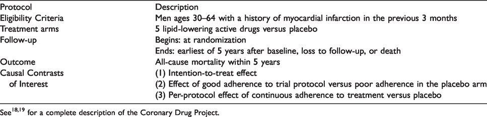
The U.S. National Heart Blood and Lung Institute sponsored the Coronary Drug Project (CDP), a double-blind placebo-controlled randomized trial conducted between 1966–75, to determine the safety and efficacy of a set of drugs for secondary prevention of mortality among men with a history of myocardial infarction.¹⁸ The trial initially compared 5 active treatments, but for simplicity we focus on the comparison between clofibrate and placebo.¹⁹ Clofibrate (no longer available in the U.S.) was a lipid-lowering agent first created in 1966 that works to increase lipoprotein lipase activity to decrease high cholesterol and triglyceride levels. In the trial, patients were instructed to take 600 mg three times per day. The placebo was sugar pills, designed to look like clofibrate, and taken on the same schedule. Adherence to treatment in this trial was defined by the physician at each quarterly visit throughout follow-up, who visually inspected the bottle of pills to describe the adherence as “good” (≥80% empty) versus “poor” (<80% empty). Table 1 presents a description of the relevant parts of the CDP.

Table 1.

Succinct description of the Coronary Drug Project.

Protocol	Description
Eligibility Criteria	Men ages 30–64 with a history of myocardial infarction in the previous 3 months
Treatment arms	5 lipid-lowering active drugs versus placebo
Follow-up	Begins: at randomizationEnds: earliest of 5 years after baseline, loss to follow-up, or death
Outcome	All-cause mortality within 5 years
Causal Contrasts of Interest	(1) Intention-to-treat effect(2) Effect of good adherence to trial protocol versus poor adherence in the placebo arm(3) Per-protocol effect of continuous adherence to treatment versus placebo

See^18,19 for a complete description of the Coronary Drug Project.

In 1980, the Coronary Drug Project team published an analysis comparing 5-year survival among individuals who did and did not adhere (at all quarterly visits) to placebo, and detected a large association between placebo adherence and survival.²⁰ The results of this study have been used to argue that adherence adjustment (and by extension, per-protocol effect estimation) cannot be done in a randomized trial. However, re-analyses of the Coronary Drug Project accounting for post-randomization confounding using inverse probability weighting showed that this association was spurious.^21,22

The CDP contains protected health information, so sharing is restricted. Instead, we have created a simulated dataset,¹⁷ based on the relationships between a subset of the variables recorded in the CDP from the clofibrate and placebo arms. The data are in long format, so each row corresponds to one person-visit. A complete data dictionary is available in eTable 1. Although some individuals in the original trial were lost to follow-up, for simplicity we have chosen to simulate data with no loss to follow-up; all individuals either contribute the full 5 years of follow-up, or follow-up ends due to death. The methodology presented here is easily extendable to scenarios with other types of censoring.

Causal thinking

Data Structure and Notation. Our simulated data structure from $T = 14$ visits takes the following structure: $O = (Z, L_{0}, A_{0}, Y_{0}, L_{1}, A_{1}, Y_{1}, \dots, L_{T}, A_{T}, Y_{T})$ , where $Z$ represents randomized treatment assignment, $A$ represents adherence to randomly assigned treatment, $L$ represents the vector of measured covariates, and $Y$ represents whether the outcome occurred in the interval $[t, t + 1)$ . Subscripts indicate time scale, for example, study visits or calendar time. We use an overbar to indicate the history of a variable up to time $t$ , e.g. adherence history at time $t$ is $\bar{A_{t}} = (A_{0}, \dots, A_{t})$ . We use lowercase values to represent a specific value, and uppercase values to represent the random variable. $Y_{t}$ is missing if the individual was lost to follow-up during $[t, t + 1)$ . We also consider $U$ , a vector of unmeasured covariates. A key point here is that to define a per-protocol effect, measures of both adherence and predictors of adherence and survival must be repeated.

Defining a causal estimand. Classically, the primary effect of interest from randomized trials is the ITT, which is the effect of randomization on the outcome of interest. The assumptions required to endow an intention-to-treat estimate from a randomized trial with a causal interpretation have been described extensively in the literature.^14,23 Briefly, these include no unmeasured confounding, no informative loss to follow-up, a non-zero probability of being randomized to each treatment arm for all participants, and a clear specification of the causal question. In general, only no informative loss to follow-up is likely to be violated in any sufficiently large randomized trial.

We are also interested in the per-protocol effect: the effect of adherence to assigned treatment strategy defined by the study protocol. Under perfect treatment strategy adherence by all trial participants, this effect is identical to the ITT. The interpretation of a per-protocol effect is therefore trial-specific, and more than one per-protocol effect definition is possible for a given trial. Researchers often estimate these effects in pragmatic trials because patients and providers want a measure of effectiveness that is not influenced by adherence. Examples of different kinds of per-protocol effects that can be estimated from survival analyses are given in Table 2.

Table 2.

Types of per-protocol effects comparing two longitudinal treatment strategies, $\bar{a}$ and $\bar{a^{*}}$ , that can be interpreted causally in a survival analysis context.

Effect type	Definition
Cumulative incidence difference/ratio at t	$RD (t) = \Pr (Y_{t}^{\bar{a}} = 1) - \Pr (Y_{t}^{\bar{a }} = 1); RR (t) = \frac{\Pr (Y_{t}^{\bar{a}} = 1)}{\Pr (Y_{t}^{\bar{a }} = 1)}$
Hazard Ratio at time t^	$HR (t) = \frac{λ^{\bar{a}} (t)}{λ^{\bar{a *}} (t)}$

$\bar{a}$ and $\bar{a^{*}}$ here are assumed to be vectors of length t.

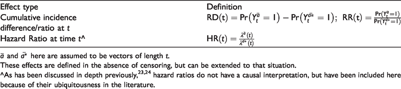
These effects are defined in the absence of censoring, but can be extended to that situation.

^As has been discussed in depth previously,^23,24 hazard ratios do not have a causal interpretation, but have been included here because of their ubiquitousness in the literature.

In order to estimate the per-protocol effect, researchers first need to define the protocol of interest. For simplicity, we will specify the static protocol: “continuously adhere to the assigned treatment arm, i.e., take at least 80% of assigned pills,” to answer the question “What is the causal effect of clofibrate versus placebo on mortality over 5 years?” As such, we are contrasting the counterfactual world where everyone took clofibrate, $\bar{a_{t}} = (1, \dots, 1)$ , to the counterfactual world where everyone took placebo, $\bar{a_{t}} = (0, \dots, 0) .$ We could also have specified a dynamic strategy such as “continuously adhere to assigned treatment arm until a pre-specified contraindication develops, after which stop taking assigned treatment arm.” To interpret an estimate as a causal per-protocol effect, there are explicit assumptions (see Box 1). Box 1.

Causal assumptions for per-protocol effects.

1. Consistency. For all $t$ and each individual who experienced adherence history $\overline{A_{t}} = \overline{a_{t}}$ , $Y_{i t}^{\overline{a_{t}}} = Y_{i t}$ – that is, the observed outcome at time t for individuals who experienced a particular adherence history $\overline{a_{t}}$ is the same as the counterfactual outcome, had we forced them to experience adherence history $\overline{a_{t}}$ . A natural check for the consistency assumption is to ensure that your intervention is well-defined, that is, each individual is receiving the same version of the treatment. Here our intervention is well defined – each individual receives 600 mg of either treatment or placebo each day – but our measure of treatment adherence easily lends itself to multiple versions.

2. Conditional exchangeability (or sequential randomization). For all $t$ , adherence histories $\overline{a_{t}}$ and covariate histories $\overline{ℓ_{t}}$ , $Y_{t}^{\overline{a_{t}}} ∐ A_{t} ∣ \overline{A_{t - 1}} = \overline{a_{t - 1}}, \overline{L_{t}} = \overline{ℓ_{t}}$ . At each time t, conditional on past adherence history and covariate history, observed adherence is independent from the counterfactual outcomes – there is no unmeasured confounding for adherence status and survival.

3. Positivity. If $f_{\overline{a_{t - 1}}, \overline{L_{t}}} (\overline{a_{t - 1}}, \overline{ℓ_{t}}) \neq 0$ , then $f_{A_{t} ∣ \overline{a_{t - 1}}, \overline{L_{t}}} (a_{t} ∣ \overline{a_{t - 1}}, \overline{ℓ_{t}}) > 0$ for all $a_{t}$ . This implies that theoretically, individuals in each subgroup defined by adherence and covariate history have non-zero probability of being both adherent and non-adherent. Practically, positivity may be violated especially if any of the $L s$ are continuous.

4. No interference. Each individual’s treatment assignment does not affect the counterfactual outcome of others, ${\overline{A}}_{i t} ∐ Y_{j t}^{\overline{a_{t}}}$ . This implies both that resource allocation is not an issue for treatment adherence, and individual’s outcomes have no bearing on what other study participant’s behavior is.

For complete discussions of these assumptions, please see.^23,30,38

Drawing the DAG. To visualize the interplay between these variables and assess the potential for bias due to confounding and selection bias, we use directed acyclic graphs (DAGs).^25,26 To avoid visual clutter, the DAGs in Figures 1 and 2 are drawn under the assumption that the null hypothesis (no effect of randomization, treatment or adherence on the outcome) is true – this is why arrows from Z to Y and from $A$ to $Y$ are absent. We also simplify the DAGs in Figure 2 (adapted from Hernan and Robins¹²) by removing any direct effect between past and future adherence (though they are still associated through other variables in the DAG) - in practice we would not make this assumption. Although we present four possible scenarios in Figure 2, here we assume that DAG C is the best representation of our trial. However, note that this is a strong assumption that is only reasonable for the CDP trial due to the rich data available on measured covariates at baseline and throughout follow-up. In trials with a placebo arm, this assumption can be partially tested by attempting to control for confounding over time between placebo arm adherers and non-adherers, in cases where the outcome is assumed to be unaffected by placebo.^21,22,27,28

Figure 1.

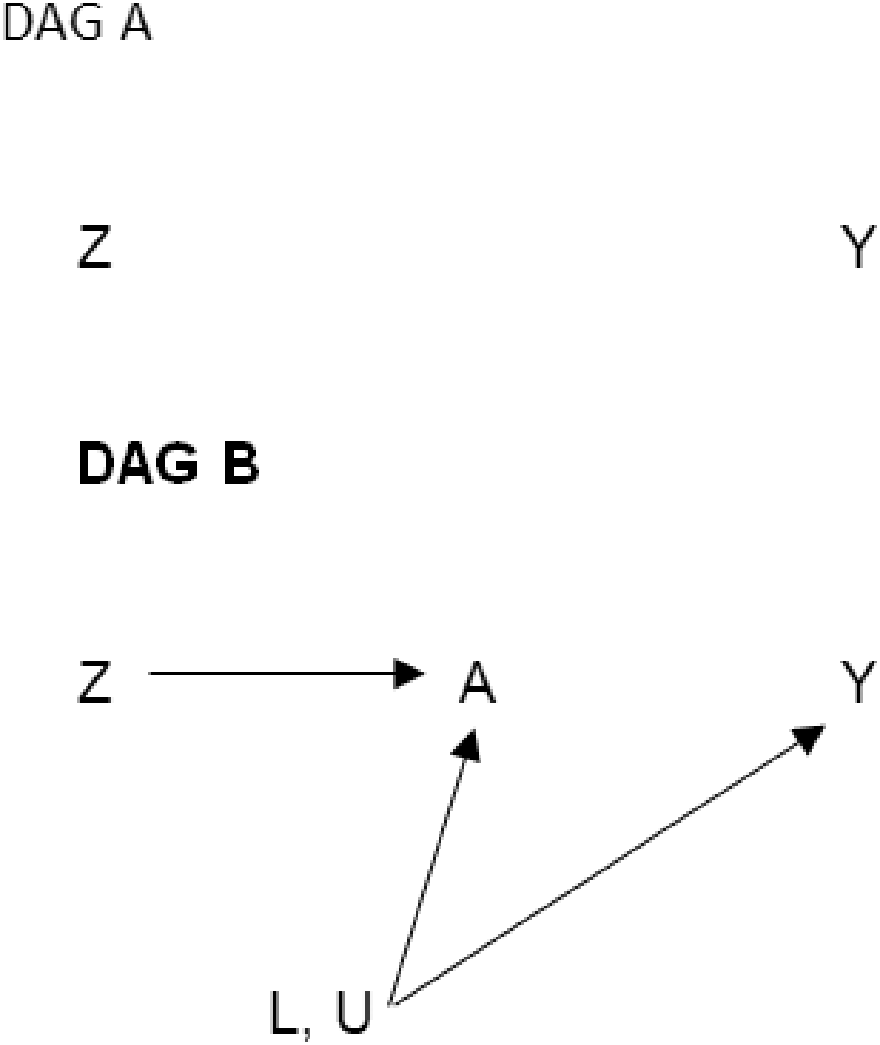
Directed acyclic graphs representing simple scenarios for estimating the intention-to-treat effect in a randomized trial. DAG A includes only Z and Y because the effect of randomization (Z) on the outcome (Y) is unconfounded by design. DAG B shows the mechanism by which the intention-to-treat effect operates. Common causes of A and Y could be measured (L) or unmeasured (U). We do not include a direct arrow from randomization (Z) to the outcome (Y) because we believe random assignment affects the outcome only through receiving treatment (A).

Figure 2.

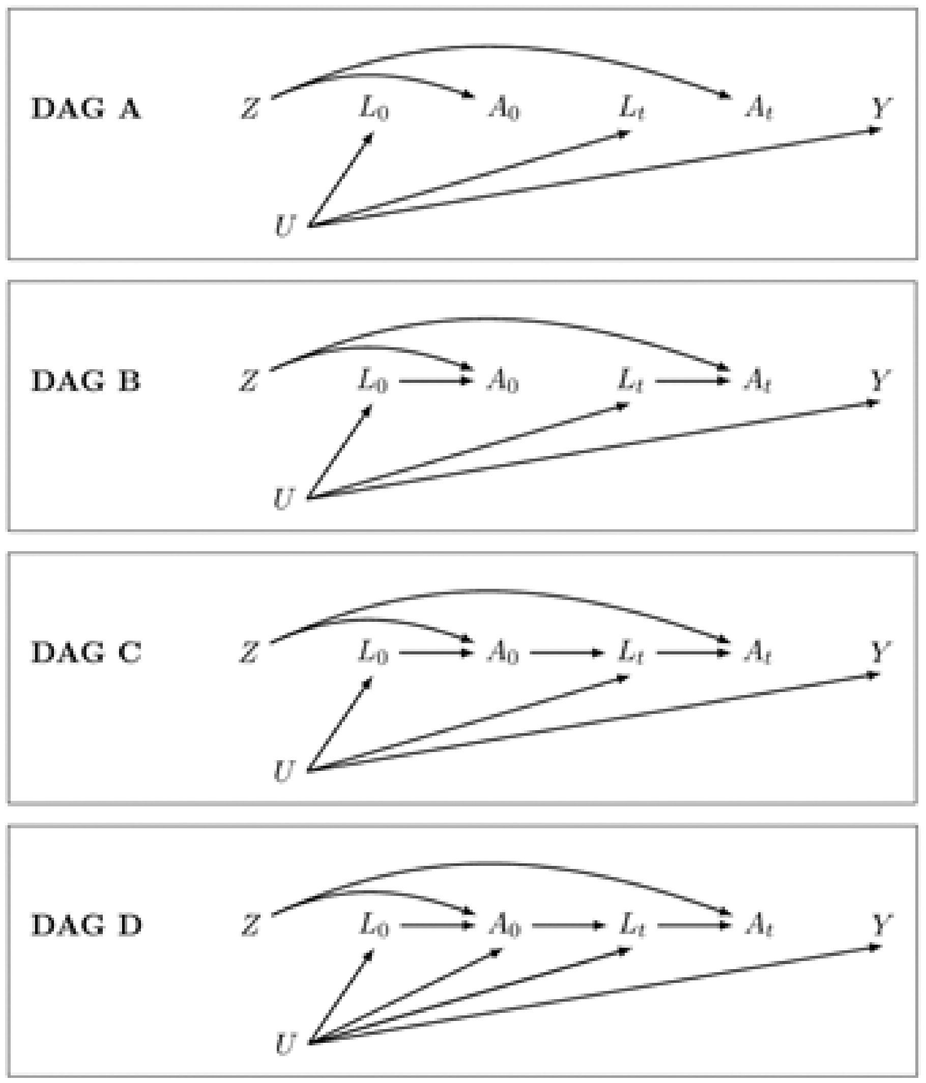
Directed acyclic graphs representing simple scenarios for estimating the per-protocol effect in a randomized trial. DAG A is drawn under the (simplistic and unrealistic) assumption that adherence is random and therefore there are no arrows from either measured or unmeasured covariates to treatment; there is no confounding or potential selection bias for the effect of treatment on the outcome, so we can use classic regression methods to estimate the per-protocol effect. DAG B imposes the assumption that the measured confounders affect adherence at each time point. In this scenario we do have time-varying confounding, but we can adjust using any statistical method (for example, adjusting for the $L s$ as time-varying confounders in a Cox proportional hazard model), because treatment-confounder feedback is absent.²⁹ DAG C builds on DAG B by additionally assuming that prior adherence also affects the measured covariates, introducing time-varying confounding and treatment-confounder feedback. Adjusting for the confounders using traditional statistical methods will open colliders at the post-baseline confounders $L_{t}$ . Even if treatment has no effect on the outcome, adjusting for $L_{t}$ using traditional statistical methods will induce an association between treatment and the outcome. Instead, to estimate the treatment-outcome effect, we need to use g-methods, such as inverse probability weighting, the g-formula, or g-estimation.^23,30–32 DAG D introduces a more extreme case, where adherence is affected by the unmeasured confounders. Now, even g-methods will generally not be sufficient to control for all the potential bias. We can still estimate the per-protocol effect in this scenario, but only by using g-estimation of structural nested models (not discussed further here).^33–37Adapted from Hernan and Robins, New England Journal of Medicine, 2017.¹²

Estimating the intention-to-treat effect

Descriptions of how to estimate unadjusted intention-to-treat hazard ratios and conditional intention-to-treat hazard ratios adjusted for baseline variables are ubiquitous in the literature. Here, we describe how to estimate standardized average counterfactual survival curves and how to use these estimates to calculate average causal effects on the hazard ratio, cumulative incidence difference, and cumulative incidence ratio scales. We outline the following six steps, also described by Hernán and Robins.²³

Fit a pooled logistic regression model with product terms: We estimate the parameters of the following pooled logistic regression model for death at visit t+1 that includes product terms between randomization arm Z and visit t:

logit [\Pr (Y_{t + 1} = 1| Z, L_{0}, {\bar{Y}}_{t} = 0)] = β_{0, t} + β_{1} Z + β_{2} L_{0} + β_{3, t} Z = β_{0}^{*} + β_{1} Z + β_{2} L_{0} + β_{3} Z t + β_{4} t + β_{5} t^{2} + β_{6} Z t^{2}

For an explanation of when and why the parameters of a pooled logistic model can be used to approximate the parameters of a Cox proportional hazards model, see Box 2. In the following steps, we will use the model’s predicted hazards p at each visit t for each value of Z and L₀:

2. Simulate data for the treated: We now create a new dataset which includes 1 copy of every person at baseline and in which everyone is assigned to treatment (Z=1). Using this dataset and the predicted hazards from step 1, we calculate the predicted survival s at each visit for each person by taking the cumulative product of each person’s conditional survival probability at each visit (1−p). This is equivalent to using the Kaplan-Meier method (s=s*(1−p)) to calculate survival.

3. Simulate data for the placebo: We repeat step 2, but assign everyone to placebo (Z=0).

4. Calculate average counterfactual survival: We now concatenate the 2 simulated datasets created in steps 2 and 3. We need to introduce some new notation for counterfactual outcomes; for an observed outcome variable Y, and an exposure variable A, the counterfactual outcome when A = a is represented by Y^a. The first simulated dataset is used to estimate counterfactual survival under treatment at each visit t, ${\hat{S}}^{z = 1} (t)$ . The second is used to estimate counterfactual survival under placebo at each visit t, ${\hat{S}}^{z = 0} (t)$ . To calculate average counterfactual survival at each visit, we average over all individuals separately for each new trial arm (treatment and placebo). This process effectively standardizes our estimates to the distribution of the baseline covariates L_0.

5. Plot counterfactual survival curves: Once we have obtained average counterfactual survival under treatment and under placebo at each visit, we can plot counterfactual survival curves.

6. Calculate hazard ratio, cumulative incidence difference, and cumulative incidence ratio: Finally, we can use the counterfactual survival estimates to calculate the average causal effect on the hazard ratio, cumulative incidence difference, and cumulative incidence ratio scales. The hazard ratio at each visit during follow-up is estimated as $\log ({\hat{S}}^{z = 1} (t)) / \log ({\hat{S}}^{z = 0} (t))$ . The cumulative incidence at each visit is calculated using the equation $1 - {\hat{S}}^{z = 1} (t)$ for the treated and $1 - {\hat{S}}^{z = 0} (t)$ for the placebo. Since our model does not make the proportional hazard assumption (we include product terms between randomization and time), we can choose what hazard ratio to estimate. One example is the average hazard ratio over the whole study period.

Box 2.

Cox proportional hazards regression versus pooled logistic regression.

Conceptual difference. Cox proportional hazard regression is a semi-parametric modeling approach – we assume that the hazard ratio is constant over follow-up and in return we do not need to make any assumptions about the functional form of the baseline hazards. If your target parameter is a conditional hazard ratio, Cox proportional hazards regression makes the fewest assumptions while giving an estimate of the hazard ratio.

λ (t∣ Z) = λ_{0} (t) e xp (λ_{1} Z)

Pooled logistic regression is a parametric modeling approach –we need to make assumptions about the functional form the baseline hazard and about whether the hazard ratio is constant or time-varying. In return, we can use the results of this model to estimate not only the hazard ratio but also the survival, cumulative incidence (risk) difference, and cumulative incidence (risk) ratio. The pooled logistic regression model estimates the discrete time hazard, so one important caveat is that we need the outcome to be rare (<10%) in each time interval.

logit [\Pr (Y_{t} = 1∣ Z)] = β_{0 t} + β_{1} Z = α_{0} + α_{1} f (t) + β_{1} Z

Implementation. To estimate the hazard ratio from a Cox proportional hazards model, we only need to know the amount of follow-up time and vital status at the end of follow-up for each individual. We also need to specify how to handle ties (individuals with events at the same time). Common methods are Breslow (used here), Efron, and exact.

To estimate the hazard ratio from a pooled logistic regression model, we need to use data in long (person-time) format. Time will be included as a covariate in our model to specify a functional form for the baseline hazard. We want to allow time to be included in a very flexible manner (e.g. polynomials, splines, categorical), as the pooled logistic regression model assumes that the baseline hazard is correctly specified. We can choose to include interaction terms between the treatment variable and time, which would relax the assumption that the treatment effect is constant over time. Moreover, the standard error estimates need to be adjusted to reflect the correlated observations. This can be achieved in two ways: (i) using a robust “sandwich” estimator, which gives valid but conservative estimates, or (ii) bootstrapping individuals to get valid, non-conservative intervals.

Estimating the per-protocol effect

Given a study protocol, there are two main approaches we can use to estimate the per-protocol effect: a censoring approach and a dose-response approach. Either determines:

whether each individual is adherent or not at baseline and then artificially censors them if and when they stop adhering, or

whether each individual is adherent or not at every time point and models adherence as a continuous variable.

Here, we use approach (a); for an example of the second approach, see.²²

To estimate our per-protocol effect, we need to control for baseline and time-varying (post-randomization) confounding of adherence and mortality. Since many of the confounders may also be affected by prior adherence, we need to use g-methods to ensure that our adjustment does not introduce additional bias.³⁰ Here, we will use an inverse probability of adherence weighted marginal structural model, outlined in the following steps:

Estimate inverse probability of adherence weights. We will use pooled logistic regression models (see Box 2) to estimate the probability of adherence weights. We estimate these weights separately in each trial arm since the reasons for non-adherence may differ between the two arms. These weights will adjust our estimates for the potential selection bias induced by the artificial censoring process, creating a pseudo-population where everyone either continuously adheres to treatment or placebo.

Estimate the working outcome model using a weighted pooled logistic regression model. Estimate the parameters of a weighted pooled logistic regression model, strictly in the person-time where individuals are continuously adherent, to get estimates in the pseudo-population.

Standardize the outcome model over baseline covariates to calculate marginal estimates. We take this step to generate estimates that are adjusted for baseline covariates, but retain their interpretation as population causal effects. Estimate counterfactual survival curves and the average hazard ratio, cumulative incidence difference, and cumulative incidence ratio at 14 visits. Calculate the average effects of interest from our survival estimates obtained via standardization.

1. Estimate inverse probability of adherence weights. To estimate the effect of adherence on all-cause mortality, we first need to create inverse probability of adherence weights. These weights will create a pseudo-population where the association between adherence and time-varying confounders is removed, allowing adherence to appear to be randomized with respect to the observed time-varying covariate distribution. There are many methods to calculate weights (unadjusted, stabilized, normalized, truncated). Stabilized weights can be estimated easily whenever we have static sustained treatment strategies or point exposures, but dynamic sustained treatment strategies require unstabilized weights.

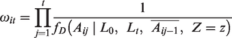
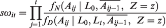
Unstabilized weights, $ω_{i t}$ , are calculated for each individual at each visit based on the predicted probability of an individual having the adherence (or exposure) they actually experienced, conditional on their baseline and time-varying covariates. These weights are similar to survey sampling weights, from the classic Horvitz-Thompson estimator³⁹

ω_{i t} = \prod_{j = 1}^{t} \frac{1}{f_{D} (A_{i j}∣ L_{0}, L_{t}, \overline{A_{i j - 1}}, Z = z)}

where, given an estimated

η_{i t} = \Pr (A_{i t} = 1∣ L_{0}, L_{t}, \overline{A_{i j - 1}}, Z = z)

f_{D} (A_{i j}∣ L_{0}, L_{t}, \overline{A_{i j - 1}}, Z = z) = A_{i t} η_{i t} + (1 - A_{i t}) η_{i t}

Stabilized weights are similar to unstabilized weights but have as a numerator the predicted probability of an individual having the adherence (or exposure) history they actually received, conditional on their baseline covariates. Stabilization ensures the weighting scheme is based only on the time-varying covariates.

{s ω}_{i t} = \prod_{j = 1}^{t} \frac{f_{N} (A_{i j} ∣ L_{0}, \overline{A_{i j - 1}}, Z = z)}{f_{D} (A_{i j} ∣ L_{0}, L_{t}, \overline{A_{i j - 1}}, Z = z)}

In this example we will use truncated stabilized weights – that is, stabilized weights which are truncated to prevent extreme values. $f_{N}$ is defined similarly to $f_{D}$ as above. Typically truncation occurs at the 99^th percentile of the weights (at all time points together), as we only wish to prevent individuals being significantly up-weighted – we do not mind if they are down-weighted to 0.

Also, note that in other settings, we may want to include adherence history in different forms in the weight models. For simplicity here, we have simply included baseline adherence ( $A_{0}$ ), and adherence at the prior visit ( $A_{t - 1}$ ), but other models could include, for example, 2-visit lagged adherence ( $A_{t - 2})$ , or cumulative adherence to time t, $\sum_{j = 0}^{t} A_{j}$ .

It is best practice to check the weight distribution – while unstabilized weights can have a mean much higher than 1, stabilized weights should have a mean of approximately 1. Truncation should reduce the mean and narrow the range of the weights.

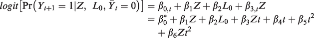
2. Estimate the working outcome model. We can now use the truncated, stabilized inverse probability of adherence weights to estimate the hazard ratio for overall mortality for our per-protocol effect. Recall our protocols are 1) continually adhere to the placebo protocol “take at least 80% of assigned placebo pills” versus 2) continually adhere to the treatment protocol “take at least 80% of assigned treatment pills”.

We will censor individuals when they deviate from their assigned protocol – that is, individuals assigned to the placebo arm are censored if and when they no longer take at least 80% of their assigned placebo pills and individuals assigned to the treatment arm are censored if and when they no longer take at least 80% of their assigned treatment pills. We then use a weighted pooled logistic regression model for the outcome. The model is the same as the model described in the ITT section above, except that it is restricted to the uncensored person-time:

logit [\Pr (Y_{t + 1} = 1| Z, {\bar{A}}_{t} = 1, L_{0}, {\bar{Y}}_{t} = 0)] = β_{0, t} + β_{1} Z + β_{2} L_{0} + β_{3, t} Z = β_{0}^{*} + β_{1} Z + β_{2} L_{0} + β_{3} Z t + β_{4} t + β_{5} t^{2} + β_{6} Z t^{2}

3. Estimating standardized survival curves. To estimate the average survival if everyone adhered to each protocol, we standardize our estimates to the baseline covariates so that our estimates can be interpreted as marginal (rather than conditional) causal effects – the survival had everyone adhered to treatment for 5 years and the survival had everyone adhered to placebo for 5 years. To do this, we use the same approach as we used to estimate the standardized ITT survival curves described in the previous section. The estimated standardized survival curves for our simulated dataset our shown in Figure 3. Table 3 shows the per-protocol causal effect over follow-up time on the hazard ratio, cumulative incidence difference, and cumulative incidence ratio scales.

Figure 3.

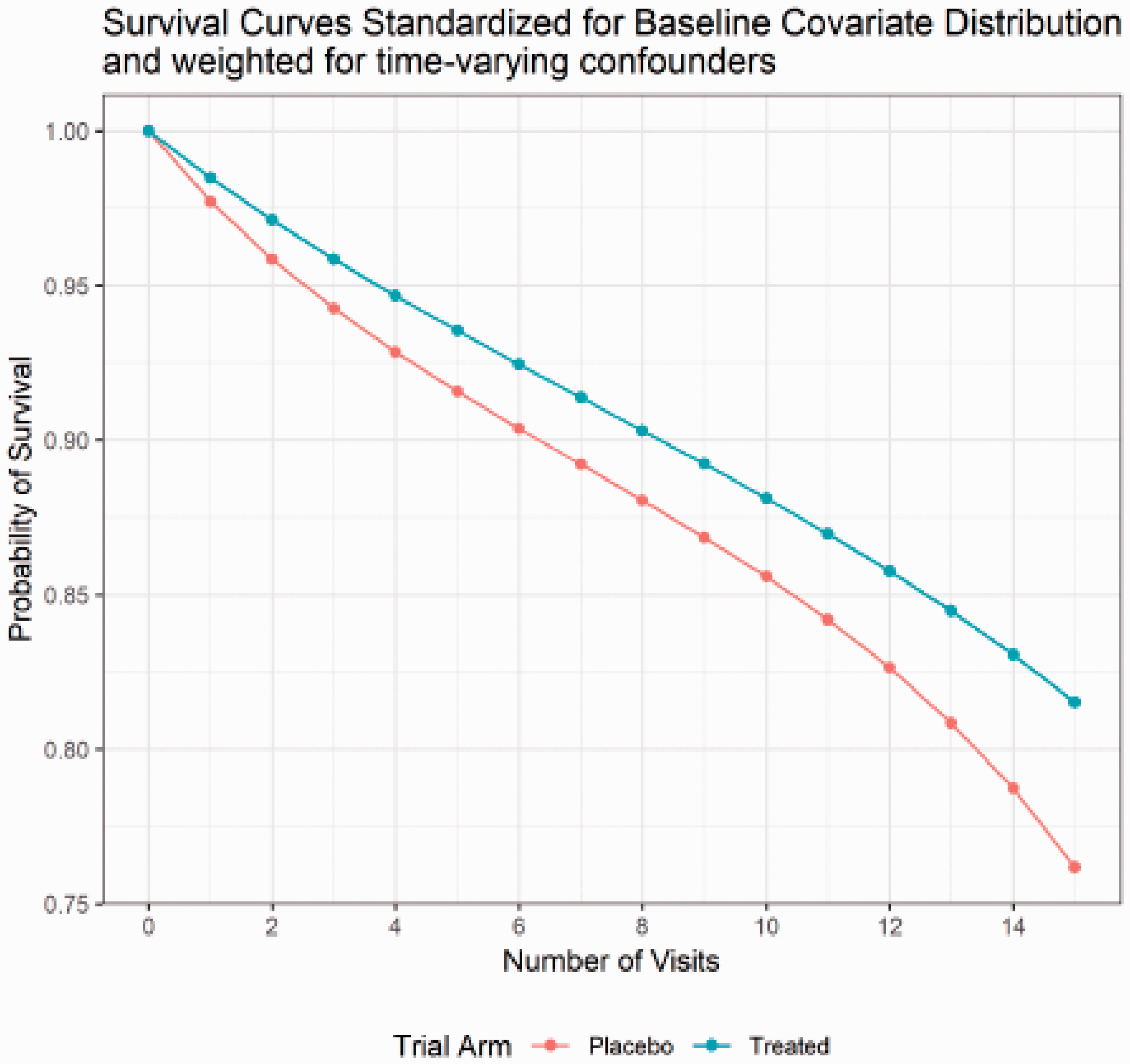
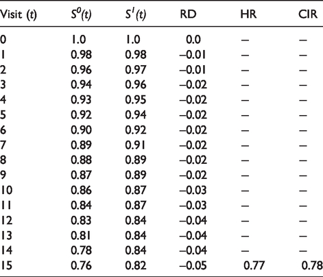
Counterfactual per-protocol survival curves standardized for baseline covariate distribution and weighted for time-varying confounders in simulated dataset.

Table 3.

Per-protocol causal effects on the hazard ratio (HR), cumulative incidence (risk) difference (RD), and cumulative incidence ratio (CIR) scales.

Visit (t)	S⁰(t)	S¹(t)	RD	HR	CIR
0	1.0	1.0	0.0	−	−
1	0.98	0.98	–0.01	−	−
2	0.96	0.97	–0.01	−	−
3	0.94	0.96	–0.02	−	−
4	0.93	0.95	–0.02	−	−
5	0.92	0.94	–0.02	−	−
6	0.90	0.92	–0.02	−	−
7	0.89	0.91	–0.02	−	−
8	0.88	0.89	–0.02	−	−
9	0.87	0.89	–0.02	−	−
10	0.86	0.87	–0.03	−	−
11	0.84	0.87	–0.03	−	−
12	0.83	0.84	–0.04	−	−
13	0.81	0.84	–0.04	−	−
14	0.78	0.84	–0.04	−	−
15	0.76	0.82	–0.05	0.77	0.78

Inference

When we use inverse probability weighting, we again need to calculate robust standard errors or use bootstrapping to get valid confidence intervals. Robust standard errors will provide conservative estimates of the confidence intervals (higher than 95% coverage), as they treat the weights as true fixed population values. Bootstrapping the entire procedure (steps 1–3) will treat the weights as estimated, providing valid confidence intervals. The procedure presented here is singly robust – that is, unbiased inference depends on the assumption that the weight model is correct. Doubly robust procedures, where either the weight model or the outcome model is correct, are available, but implementation is not so straightforward.^40,41

Extensions to observational studies

The main difference between causal survival analysis in RCTs or other experiments compared to observational studies is baseline confounding. Here we derived our example from a real randomized trial. However, the reader may be interested in implementing these ideas to study the effect of an exposure on a time-to-event outcome in observational data. There are two additional challenges to consider in causal survival analysis from observational studies: identification of time zero, and well-defined interventions. In RCTs, we know both when follow-up begins (time zero) and exactly which treatments are being compared because we assign individuals to treatment. However, in observational studies exposure is not assigned, leading to issues with time zero and the consistency assumption from causal inference. The target trial framework provides guidance for designing a study and analysis where the potential for bias in the choice of time zero and ambiguity in interpretation because of a lack of well-defined interventions is minimized.^42–44 Briefly, the target trial framework requires us to imagine a hypothetical randomized trial to answer our scientific question, and use this to design our observational study. Using this methodology, we can frame scientific questions regarding the effect of a longitudinal exposure on a time-to-event outcome arising from observational data.

Conclusion

Randomized clinical trials are an ideal tool for estimating the causal effect of a potentially beneficial intervention. However, whenever any participants do not adhere perfectly to their treatment assignment, the interpretation of these trials can be complicated. With this tutorial, we hope to provide practical guidance on how to use modern causal inference techniques to estimate the per-protocol effect of a longitudinal treatment on a survival outcome.

All attempts to estimate causal effects require strong assumptions – even the ITT effect. In the case of the ITT, the most commonly violated assumption is that of no informative loss to follow-up. In RCTs with loss to follow-up, a similar approach to that described here for adjusting for non-adherence can be used to adjust for informative loss to follow-up, but only when predictors of loss to follow-up that are also prognostic for the outcome have been measured in trial participants.

When the per-protocol effect is of interest, we encourage trialists to also consider conducting and presenting a range of sensitivity analyses. When the comparator treatment is placebo and if experts agree that the placebo truly has no effect on the outcome of interest, one useful sensitivity analysis is to compare adherers to non-adherers in the placebo arm using the methods described above for estimating the per-protocol effect, but replacing randomization status with adherence status.^21,22,27,28 Although such an analysis cannot guarantee that the required causal inference assumptions are met, it can be used to detect situations in which the required assumptions are clearly violated.

In this tutorial, we focused on explaining the estimation of the per-protocol effect in a simple case, where the longitudinal treatment has a single approved dose, adherence is measured as a binary variable, treatment cessation is not allowed for any reason, and there is no loss to follow-up and no competing events. Methods exist to address all of these complexities, but are beyond the scope of the current tutorial. For an overview of the conceptual approaches to dealing with those challenges, we encourage readers to refer to.¹⁴

Footnotes

Authors’ contributions

We wrote this article to disseminate and facilitate the implementation of modern causal inference methods for survival analysis to a general public health practitioner audience. E.J.M., E.C.C., and L.C.P. developed the concept and wrote the article. E.J.M. wrote the SAS and Stata code. L.C.P. and E.J.M. wrote the R code. All authors drafted and revised the both manuscript and the code. All authors read and approved the final version of the manuscript. E.J.M. and L.C.P. are the guarantors of the article.

Acknowledgments

We thank Roger W Logan for his help creating the simulated dataset. We thank Miguel Hernán for helpful feedback on an earlier version of this work.

Declaration of Conflicting Interests

The author(s) declared no potential conflicts of interest with respect to the research, authorship, and/or publication of this article.

Funding

The author(s) received no financial support for the research, authorship, and/or publication of this article.

ORCID iD

Lucia C Petito

References

US Food & Drug Administration. E9: statistical principles for clinical trials. Fed Regist 1998; 63: 49583–49598.

Collett

Modelling survival data in medical research. New York: Chapman and Hall/CRC, 2014.

Piantadosi

Clinical trials: a methodologic perspective. 2nd ed. Hoboken, NY: Wiley-Interscience, 2005.

Rosenberger

Lachin

JM.

Randomization in clinical trials: theory and practice. New York, NY: Wiley-Interscience, 2002.

Singh

Mukhopadhyay

Survival analysis in clinical trials: basics and must know areas. Perspect Clin Res 2011; 2: 145–148.

Cox

DR.

Regression models and life tables. J R Stat Soc Ser B (Methodol) 1972; 34: 187–220.

Hernán

Hernandez-Diaz

Robins

JM.

Randomized trials analyzed as observational studies. Ann Intern Med 2013; 159: 560–562.

Kaplan

Meier

Nonparametric estimation from incomplete observations. J Am Stat Assoc 1958; 53: 457–481.

Kleinbaum

Klein

Survival analysis: a self-learning text. 3rd ed. New York, NY: Springer, 2012.

10.

Bertolini

Bon

Campbell

, et al. Efficacy and safety of atorvastatin compared to pravastatin in patients with hypercholesterolemia. Atherosclerosis 1997; 130: 191–197.

11.

Moore

Goldstein

Hamm

, et al. Erlotinib plus gemcitabine compared with gemcitabine alone in patients with advanced pancreatic cancer: a phase III trial of the national cancer institute of Canada clinical trials group. J Clin Oncol 2007; 25: 1960–1966.

12.

Hernán

Robins

JM.

Per-Protocol analyses of pragmatic trials. N Engl J Med 2017; 377: 1391–1398.

13.

Hernán

Hernandez-Diaz

Beyond the intention-to-treat in comparative effectiveness research. Clin Trials 2012; 9: 48–55.

14.

Murray

Swanson

Hernán

MA.

Guidelines for estimating causal effects in pragmatic randomized trials. 2019; arXiv:1191.06030v2[stat.ME].

15.

Murray

Caniglia

Swanson

, et al. Patients and investigators prefer measures of absolute risk in subgroups for pragmatic randomized trials. J Clin Epidemiol 2018; 103: 10–21.

16.

Rudolph

Naimi

Westreich

, et al. Defining and identifying per-protocol effects in randomized trials. Epidemiology 2020; 31: 692–694.

17.

Murray

Petito

CausalSurvivalAnalysisWorkshop V1.0. Zenodo, http://doi.org/10.5281/zenodo.3990592 (accessed 10 September 2020).

18.

Coronary Drug Project Research Group. The Coronary Drug Project: design, methods, and baseline results. Circulation 1973; 47: l–1.

19.

Coronary Drug Project Research Group. Clofibrate and niacin in coronary heart disease. J Am Med Assoc 1975; 231: 360–381.

20.

Coronary Drug Project Research Group. Influence of adherence to treatment and response of cholesterol on mortality in the Coronary Drug Project. N Engl J Med 1980; 303: 1038–1041.

21.

Murray

Hernán

MA.

Adherence adjustment in the Coronary Drug Project: a call for better per-protocol effect estimates in randomized trials. Clin Trials 2016; 13: 372–378.

22.

Murray

Hernán

MA.

Improved adherence adjustment in the Coronary Drug Project. Trials 2018; 19: 158.

23.

Hernán

Robins

JM.

Causal inference: what if? Boca Raton: CRC, 2020.

24.

Hernán

MA.

The hazards of hazard ratios. Epidemiology 2010; 21: 13–15.

25.

Greenland

Pearl

Robins

JM.

Causal diagrams for epidemiologic research. Epidemiology 1999; 10: 37–48.

26.

Pearl

Introduction to probabilities, graphs, and causal models. In: Causality: models, reasoning, and inference. Cambridge, UK: Cambridge University, 2000, pp.1–40.

27.

Murray

Claggett

Granger

, et al. Adherence-adjustment in placebo-controlled randomized trials: an application to the candesartan in heart failure randomized trial. Contemp Clin Trials 2020; 90: 105937.

28.

Wanis KN, Madenci AL, Hern´n MA, Murray EJ. Adjusting for adherence in randomized trials when adherence is measured as a continuous variable: An application to the Lipid Research Clinics Coronary Primary Prevention Trial. Clinical Trials. May 2020. doi:10.1177/1740774520920893.

29.

Zhang

Reinikainen

Adeleke

, et al. Time-varying covariates and coefficients in cox regression models. Ann Transl Med 2018; 6: 121.

30.

Robins

Hernán

MA.

Estimation of the causal effects of time-varying exposures. In: Garrett Fitzmaurice, Marie Davidian, Geert Verbeke, Geert Molenberghs. Boca Raton, FL (eds) Longitudinal data analysis. Vol. 553, 2009, p.599.

31.

Daniel

Cousens

De Stavola

, et al. Methods for dealing with time-dependent confounding. Stat Med 2013; 32: 1584–1618.

32.

Naimi

Cole

Kennedy

EH.

An introduction to g methods. Int J Epidemiol 2017; 46: 756–762.

33.

Hernán

Cole

Margolick

, et al. Structural accelerated failure time models for survival analysis in studies with time-varying treatments. Pharmacoepidemiol Drug Saf 2005; 14: 477–491.

34.

Witteman

D'Agostino

Stijnen

, et al. G-estimation of causal effects: isolated systolic hypertension and cardiovascular death in the Framingham heart study. Am J Epidemiol 1998; 148: 390–401.

35.

Robins

JM.

The analysis of randomized and non-randomized AIDS treatment trials using a new approach to causal inference in longitudinal studies. In: Sechrest L, Freeman H, Mulley A (eds) Health service research methodology: a focus on AIDS. Washington: U.S. Public Health Service, 1989, pp.113–159.

36.

Robins

JM.

Estimation of the time-dependent accelerated failure time model in the presence of confounding factors. Biometrika 1992; 79: 321–334.

37.

Robins

Tsiatis

AA.

Semiparametric estimation of an accelerated failure time model with time-dependent covariates. Biometrika 1992; 79: 311–319.

38.

Rubin

DB.

Estimating causal effects of treatments in randomized and non-ranodmized studies. J Educ Psychol 1974; 66: 688–701.

39.

Horvitz

Thompson

DJ.

A generalization of sampling without replacement from a finite universe. J Am Stat Assoc 1952; 47: 663–685.

40.

Stitelman OM, De Gruttola V, van der Laan MJ. A general implementation of TMLE for longitudinal data applied to causal inference in survival analysis. Int J Biostat 2012; 8(1).

41.

Bang

Robins

JM.

Doubly robust estimation in missing data and causal inference models. Biometrics 2005; 61: 962–973.

42.

Hernan

Sauer

Hernandez-Diaz

, et al. Specifying a target trial prevents immortal time bias and other self-inflicted injuries in observational analyses. J Clin Epidemiol 2016; 79: 70–75.

43.

Lodi

Phillips

Lundgren

, et al. Effect estimates in randomized trials and observational studies: comparing apples with apples. Am J Epidemiol 2019; 188: 1569–1577.

44.

Labrecque

Swanson

SA.

Target trial emulation: teaching epidemiology and beyond. Eur J Epidemiol 2017; 32: 473–475.

Causal survival analysis: A guide to estimating intention-to-treat and per-protocol effects from randomized clinical trials with non-adherence

Abstract

Keywords

Introduction

Motivating example: The Coronary Drug Project

Causal thinking

Estimating the intention-to-treat effect

Estimating the per-protocol effect

Inference

Extensions to observational studies

Conclusion

Footnotes

Authors’ contributions

Acknowledgments

Declaration of Conflicting Interests

Funding

ORCID iD

References