Assessing the impact of case-mix heterogeneity in individual participant data meta-analysis: Novel use of I 2 statistic and prediction interval

Abstract

Case mix differences between trials form an important factor that contributes to the statistical heterogeneity observed in a meta-analysis. In this paper, we propose two methods to assess whether important heterogeneity would remain if the different trials in the meta-analysis were conducted in one common population defined by a given case-mix. To achieve this goal, we first standardize results of different trials over the case-mix of a target population. We then quantify the amount of heterogeneity arising from case-mix and beyond case-mix reasons by using corresponding I² statistics and prediction intervals. These new approaches enable a better understanding of the overall heterogeneity between trial results, and can be used to support standard heterogeneity assessments in individual participant data meta-analysis practice.

Introduction

Meta-analyses (MA) summarize the effectiveness of an experimental intervention compared to a control into a so-called pooled effect.^1–4 Such pooled effect can be difficult to interpret when there is important clinical and methodological heterogeneity between studies. One important step in every systematic review therefore involves the consideration of whether it is appropriate to pool results of all, or perhaps some, of the individual studies.^1,2,5 In practice, however, even when the studies have enough in common to justify evidence synthesis, residual differences between studies may still remain and impact the summary result. The random-effect meta-analysis model is frequently used to account for this heterogeneity. It acknowledges that the true effect size may vary from one study to the next, by viewing the treatment effects from the considered studies as a random sample of effect sizes that could have been observed. The variation in true effect sizes is then explored by standard heterogeneity assessment approaches, mostly by subgroup analysis and meta-regression.^1,2,5–7 These approaches may provide important insights into the possible reasons of the observed heterogeneity. However, they are often underpowered to detect differences and do not quantify how much heterogeneity is due to true variation in case mix and how much is due to other clinical factors or unknown causes of biases. ⁷ Moreover, by focusing on subgroup effects, these approaches deliver treatment effects whose magnitude may fail to be comparable with that observed in the original (unadjusted) meta-analysis.^8,9

In conventional meta-analysis, heterogeneity assessment is often supported by two statistics—the I² statistic and the prediction interval.^10,11 Originally proposed by Higgins et al, ¹⁰ the I² statistic quantifies the proportion of the total heterogeneity that is not due to sampling error in the standard random-effect meta-analyses. This is attractive in that I² statistics obtained from MAs with different numbers of studies and different effect metrics are directly comparable. This statistic is sometimes criticized, however, as being difficult to interpret for clinical readers. Besides, as the I² statistic only contrasts the standard deviation across studies with the typical standard errors of the observed effect sizes in the individual studies, its value also depends on the sample size of the eligible trials. This can mislead the overall heterogeneity assessment. For instance, large trials with slightly different effect sizes result in high I², when small trials with substantially different effect sizes can result in an I² close to zero.^11,12 Recently, the prediction interval has been considered as an alternative to represent between-trial heterogeneity.^11,13 This interval allows one to predict where the result of a new trial can be expected with a pre-specified chance, given the heterogeneity observed between the available trials.

In this paper, we extend the I² statistic and the prediction interval to enable a decomposition of the overall heterogeneity among trial results into what we term case-mix and beyond case-mix heterogeneity. To achieve this, we first provide an inverse probability weighting (IPW) approach which uses the individual participant data of all trials to standardize results of different studies over the case-mix of a target population. This approach is then extended with the aim to improve efficiency and robustness against model misspecification. Once trial results are standardized, a new class of random-effect meta-analysis models can then be fitted. These new models involve two random effects to reflect two different sources of heterogeneity, namely case-mix and beyond case-mix heterogeneity. The extension of the I² statistic and the prediction interval to this new class of models is discussed and illustrated via simulation. The proposed approaches are also applied to a real individual patient data meta-analysis evaluating anti-hypertensive treatments. Finally, we end with a concluding discussion and suggestions for future research.

Case-mix standardization in meta-analysis

Case-mix standardization has been popular in epidemiology since the 1980s, mostly with the aim of comparing mortality and morbidity rates in two or more different geographic areas.^14,15 As a naive comparison between crude rates of these areas could be misleading if the population structure in the geographic areas is different, case-mix standardization has been used to adjust for characteristic(s) that are differentially distributed across the populations (mostly age and sex).^14,15 In this section, we discuss the applicability of this technique in meta-analysis, which may likewise suffer from case mix heterogeneity between trials. This discussion makes use of counterfactual outcome theory and is inspired by our previous work and the work of Bareinboim and Pearl on non-transportability.^9,16–19

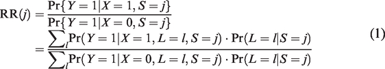
Consider a meta-analysis of K randomized controlled trials (RCTs) evaluating the comparative effectiveness of two treatments (X = 0, 1) on a dichotomous outcome Y. Assume that the randomization ratio is 1:1 across all studies. Let S be an indicator of the study from which a given patient originates (S = 1 to K) and L be a vector of baseline covariates that are prognostic for the outcome Y and are reported across the studies. The treatment effect in study S = j can then be expressed on the relative risk scale as:

$$\begin{array}{l}\text{RR}(j)=\frac{\mathrm{Pr}\{Y=1|X=1,S=j\}}{\mathrm{Pr}\{Y=1|X=0,S=j\}}\\ =\frac{{\displaystyle {\sum }_l\mathrm{Pr}}(Y=1|X=1,L=l,S=j)·\mathrm{Pr}(L=l|S=j)}{{\displaystyle {\sum }_l\mathrm{Pr}}(Y=1|X=0,L=l,S=j)·\mathrm{Pr}(L=l|S=j)}\end{array}$$

(1)

This equation makes clear that the observed variation among trial results can be explained by two factors other than chance. The first one is the variability in terms of case-mix (i.e. the study-specific distribution $\mathrm{Pr}(L=l|S=j)$ ) across the K studies. This source of heterogeneity arises, for instance, when one trial in the meta-analysis recruits patients aged 30 to 60 years, of which 50% are female, while the other trial evaluates patients (with the same condition) aged 20 to 50 years, of which 70% are female. Apart from case-mix, the observed heterogeneity among $\widehat{\text{RR}}(j)$ may also originate from methodological inconsistencies among studies, including variations of the non-pharmacological interventions in non-drug trials, differences in patient management, in attrition risk or even in outcome definition and measurement. This second source of heterogeneity is termed beyond case-mix heterogeneity and is reflected through the difference in the outcome generating mechanism $\mathrm{Pr}(Y=1|X=x,L=l,S=j)$ (x = 0, 1) across studies. As an example, consider a meta-analysis in which patient blinding is implemented in some studies (e.g. trial S = 1) but not in the others, and assume that this is the only remarkable methodological difference across the trials. One may then postulate an outcome model in which the interaction between the treatment and the study indicator is permitted, e.g. $\text{logit }\mathrm{Pr}(Y=1|X,L,S)={\beta }_0+{\beta }_1·X+{\beta }_2·L+{\beta }_3·X·I(S=1)$ where logit p = p/(1-p). Such interaction implies that the estimated treatment effect (on the logit scale) in the trial with blinding may be different from that in other trials without blinding. This may give rise the so-called beyond case-mix heterogeneity and can be detected by the approaches discussed below.

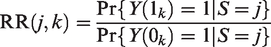
To make clear the distinction between case-mix and beyond case-mix heterogeneity, we now use $1_k$ and $0_k$ to denote the versions of treatment and control used in study k, for k = 1 to K, respectively. Besides, we denote $Y(1_k)$ and $Y(0_k)$ the binary counterfactual outcome that would be observed for a given individual if (version of) treatment/control k were administered. Under the so-called consistency assumption 9, $Y(x_k)$ equals the observed outcome Y if the considered patient originates from study S = k and is assigned to treatment arm $x_k(=0,1)$ . Furthermore, as the K trials are judged to be similar on the Population, Intervention, Control, Outcome (PICO) basis, it should be plausible to assume a positivity assumption which states that any individual with characteristics L in one study is eligible for participation in the other studies, which implies $0<\mathrm{Pr}(S=k|L)<1$ for all k = 1 to K. ⁹ Our focus is on estimating the relative risk:

$$\text{RR}(j,k)=\frac{\mathrm{Pr}\{Y(1_k)=1|S=j\}}{\mathrm{Pr}\{Y(0_k)=1|S=j\}}$$

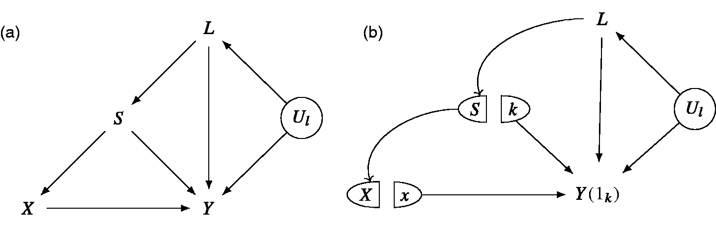
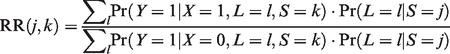
which stands for the treatment effect that would be observed if the trial k were conducted in the population of trial j. Note that other effect measures like risk differences and odds ratios can be defined in a similar way. To estimate RR(j, k), we further assume that the baseline covariate vector L contains all predictors of the outcome that are differentially distributed between studies. ⁹ Such an assumption implies that both $Y(1_k)$ and $Y(0_k)$ are independent of S given L. In practice, one important challenge could be that information on some baseline covariates is collected in some studies but not in the others. In such case, imputation methods might be needed to impute the missing covariate data (see for instance the methods proposed by Quartagno et al ²⁰ and Resche-Rigon et al ²¹ ). In Figure 1, we depict a causal diagram in which the above assumption that $Y(x_k)$ is independent of S given L is satisfied.

Figure 1.

(a) Causal diagram and (b) the corresponding Single-World Intervention Graph when X and S are set at x and k, respectively. The arrow from S to X reflects the fact that different studies may have a different randomization ratio, while the arrow from S to Y reflects methodological differences between studies that can impact the outcome. U_l: (unmeasured) predictors of the outcome Y that do not differentially distributed across studies.

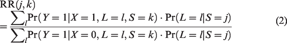
Under the aforementioned assumptions, it can be shown that:

$$\begin{array}{l}\text{RR}(j,k)\\ =\frac{{\displaystyle {\sum }_l\mathrm{Pr}}\left(Y=1|X=1,L=l,S=k\right)·\mathrm{Pr}\left(L=l|S=j\right)}{{\displaystyle {\sum }_l\mathrm{Pr}}\left(Y=1|X=0,L=l,S=k\right)·\mathrm{Pr}\left(L=l|S=j\right)}\end{array}$$

(2)

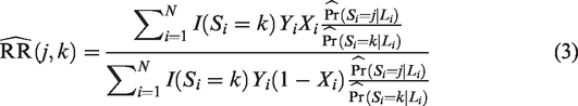
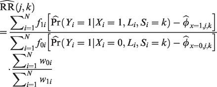
Formula (2) connects $\text{RR}(j,k)$ with the idea of case-mix standardization discussed above. Indeed, $\text{RR}(j,k)$ amounts to a simple recalibration (or reweighting) of the L-specific effects in trial k to account for the new distribution of L in trial j (which is also the underlying mechanism of case-mix standardization).^9,18 Note that $\text{RR}(j,j)$ is equivalent to the above $\text{RR}(j)$ defined by (1). A plug-in estimator of $\text{RR}(j,k)$ is then obtained by substituting the different probabilities involved in equation (2) by (consistent) estimators. A drawback of this approach is that it comes with a high risk of undiagnosed extrapolation when patients in different studies have very different case mix. ⁹ In view of this, we alternatively consider an inverse probability weighting (IPW) approach:

$$\widehat{\text{RR}}(j,k)=\frac{{\displaystyle {\sum }_{i=1}^{N}I}(S_i=k)Y_i{X}_i\frac{\widehat{\mathrm{Pr}}(S_i=j|L_i)}{\widehat{\mathrm{Pr}}(S_i=k|L_i)}}{{\displaystyle {\sum }_{i=1}^{N}I}(S_i=k)Y_i(1-X_i)\frac{\widehat{\mathrm{Pr}}(S_i=j|L_i)}{\widehat{\mathrm{Pr}}(S_i=k|L_i)}}$$

(3)

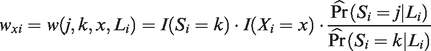
where N denotes the number of patients in the meta-analysis and $I(·)$ denotes the indicator function which satisfies $I(S=k)=1$ if S = k and 0 otherwise. This IPW approach requires a propensity score model to predict the probability of being in a given trial provided the covariate profile, i.e. $\mathrm{Pr}(S=j|L)$ . The outcome of each patient in trial k is then reweighted by the ratio $\widehat{\mathrm{Pr}}(S=j|L)/\widehat{\mathrm{Pr}}(S=k|L)$ before being used to compute the relative risk. When the propensity score model is correctly specified, the proposed inverse weighting approach yields no bias in estimating $\text{RR}(j,k)$ (when the sample size is large). The variance of this estimator can be estimated using sandwich estimators or bootstrap sampling.

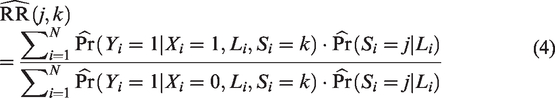
While the IPW approach has the advantage of avoiding assumptions on the degree of effect heterogeneity between populations, it is generally less efficient than the plug-in approach (see the Online Supplemental Material file S1 for a formal proof). To remedy this, IPW can be further improved by using control variates—a variance reduction technique commonly used in Monte Carlo simulation (see the Online Supplemental Material file S2). When the randomization ratio is 1:1 across all studies, the resulting augmented IPW (AIPW) estimator for $\text{RR}(j,k)$ can be expressed as:

$$\begin{array}{l}\widehat{\text{RR}}(j,k)\\ =\frac{{\displaystyle {\sum }_{i=1}^N\widehat{\mathrm{Pr}}}(Y_i=1|X_i=1,L_i,S_i=k)·\widehat{\mathrm{Pr}}(S_i=j|L_i)}{{\displaystyle {\sum }_{i=1}^N\widehat{\mathrm{Pr}}}(Y_i=1|X_i=0,L_i,S_i=k)·\widehat{\mathrm{Pr}}(S_i=j|L_i)}\end{array}$$

(4)

where the outcome prediction $\widehat{\mathrm{Pr}}(Y_i=1|X_i=x,L_i,S_i=k)$ for x = 0, 1 are estimated based on a canonical generalized linear model, using the data of (un)treated patients in trial k, with the outcome of individual i weighted by $\frac{\widehat{\mathrm{Pr}}(S_i=j|L_i)}{\widehat{\mathrm{Pr}}(S_i=k|L_i)}$ . As for IPW, the variance of the AIPW estimator can be estimated using sandwich estimators or bootstrap sampling. If the propensity score model $\mathrm{Pr}(S=k|L)$ is correctly specified, the AIPW estimator will be unbiased (when the sample size is large), and will have no larger asymptotic variance than the IPW estimator in estimating $\text{RR}(j,k)$ when the outcome model $\mathrm{Pr}(Y=1|X=x,L,S=k)$ involved in the AIPW estimator is correctly specified (and often even when it is incorrectly specified). In Appendix 1, we conduct a simulation study to illustrate this point.

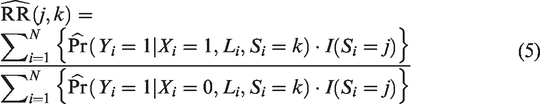
A common limitation of the above estimators is that they require either the outcome model (i.e. the plug-in approach) or the propensity score model (i.e. the IPW and AIPW approaches) to be correctly specified. To overcome the need for choosing between these two working models, one could consider the so-called doubly-robust (DR) estimators,^22,23 which can maintain validity when either one, but not necessarily both of these models is correctly specified. Such DR estimator is obtained by replacing the fitted value $\widehat{\mathrm{Pr}}(S_i=j|L_i)$ by the indicator function $I(S_i=j)$ , that is:

$$\begin{array}{l}\widehat{\text{RR}}(j,k)=\\ \frac{{\displaystyle {\sum }_{i=1}^N\left\{\widehat{\mathrm{Pr}}\left(Y_i=1|X_i=1,L_i,S_i=k\right)·I\left(S_i=j\right)\right\}}}{{\displaystyle {\sum }_{i=1}^N\left\{\widehat{\mathrm{Pr}}\left(Y_i=1|X_i=0,L_i,S_i=k\right)·I\left(S_i=j\right)\right\}}}\end{array}$$

(5)

where the outcome prediction $\widehat{\mathrm{Pr}}(Y_i=1|X_i=x,L_i,S_i=k)$ for x = 0, 1 are estimated based on a canonical generalized linear model, using the data of (un)treated patients in trial k, with the outcome of individual i weighted by $\frac{\widehat{\mathrm{Pr}}(S_i=j|L_i)}{\widehat{\mathrm{Pr}}(S_i=k|L_i)}$ . When this outcome model is incorrectly specified, the DR estimator remains asymptotically unbiased provided that the PS model is correctly specified. In contrast, when the outcome model but not the PS model is correctly specified, the DR estimator still remains valid. In the Online Supplemental Material file S3 and Appendix 1, we provide a formal proof for these properties of the DR estimator and illustrate them via a small simulation study.

It is worth noting that in the causal inference literature, the two terms AIPW and DR are often used interchangeably, as the AIPW estimator for the average treatment effect in a single study is also doubly robust. However, it has been shown that for the average treatment effect among the treated (ATT) (also in a single study setting), there are two AIPW estimators achieving local efficiency of different types, i.e. local nonparametric efficiency and semiparametric efficiency, and not both are doubly robust. Indeed, the locally nonparametric efficient estimator of the ATT is doubly robust, but the locally semiparametric efficient estimator is generally not.^24–26 In the current meta-analysis context, the standardized relative risk $\text{RR}(j,k)$ is somewhat of the same nature as the ATT in a single study, since $\text{RR}(j,k)$ expresses the treatment effect in the subgroup of patients coming from trial S = j, assuming a mega-population obtained by combining all trial populations in the meta-analysis. As in the case of the ATT, there will be two AIPW estimators achieving local efficiency of different types. The estimator that we label AIPW in the paper is locally semiparametric efficient and not doubly robust. In contrast, the so-called DR estimator for $\text{RR}(j,k)$ is locally nonparametric efficient and doubly robust. With this in mind, note that the semiparametric efficiency bound obtained by the AIPW estimator for $\text{RR}(j,k)$ is of no larger magnitude than the nonparametric efficiency bound obtained by the DR approach for the same $\text{RR}(j,k)$ . This explains why the AIPW approach with a correctly specified propensity score model will have no larger asymptotic variance than that of the DR approach, when both the propensity score and outcome model are correctly specified. A more detailed discussion on local semiparametric and nonparametric efficiency, and its impact on the double robustness of the estimator can be found elsewhere.^24–26

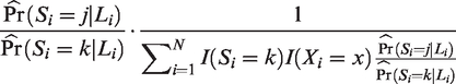
As a final remark, note that the IPW, AIPW and the DR approach can be susceptible to the presence of unstable weights, that is, to some weights $\frac{\widehat{\mathrm{Pr}}(S_i=j|L_i)}{\widehat{\mathrm{Pr}}(S_i=k|L_i)}$ being very large for some individuals. ⁹ These extreme weights can lead to a huge reduction in effective sample size, causing unstable results. For instance, on the probability scale, the IPW estimates for $\mathrm{Pr}(Y(x_k)=1|S=j)$ can be larger than 1 for certain values of j and k due to extreme weights. To remedy this, one can stabilize the weights involved in the IPW and AIPW approaches by dividing each individual weight by the sum of the weights. For the AIPW approach, this implies that the relative risk $\text{RR}(j,k)$ can be estimated by equation (4), using a canonical generalized linear outcome model for $\mathrm{Pr}(Y_i=1|X_i=x,L_i,S_i=k)$ for x = 0, 1, fitted to the data of (un)treated patients in trial k, weighting each individual i by the stabilized weight:

$$\frac{\widehat{\mathrm{Pr}}(S_i=j|L_i)}{\widehat{\mathrm{Pr}}(S_i=k|L_i)}·\frac{1}{{\displaystyle {\sum }_{i=1}^{N}I}(S_i=k)I(X_i=x)\frac{\widehat{\mathrm{Pr}}(S_i=j|L_i)}{\widehat{\mathrm{Pr}}(S_i=k|L_i)}}$$

Such a strategy can lead to bias, however, when the PS model is incorrectly specified. It hence does not maintain the double robustness property of the DR approach. Alternatively, to avoid the impact of extreme weights on the DR approach, one may consider the weight-stabilized DR estimator: ²⁷

$$\begin{array}{l}\widehat{\text{RR}}(j,k)\\ =\frac{{\displaystyle {\sum }_{i=1}^N{f}_{1i}}\left[\widehat{\mathrm{Pr}}(Y_i=1|X_i=1,L_i,S_i=k)-{\widehat{\varphi }}_{x=1,j,k}\right]}{{\displaystyle {\sum }_{i=1}^N{f}_{0i}}\left[\widehat{\mathrm{Pr}}(Y_i=1|X_i=0,L_i,S_i=k)-{\widehat{\varphi }}_{x=0,j,k}\right]}\\ ·\frac{{\displaystyle {\sum }_{i=1}^N{w}_{0i}}}{{\displaystyle {\sum }_{i=1}^N{w}_{1i}}}\end{array}$$

where $f_{xi}=w_x{Y}_i+[I(S_i=j)-w_{xi}]$ ,

$$w_{xi}=w(j,k,x,L_i)=I(S_i=k)·I(X_i=x)·\frac{\widehat{\mathrm{Pr}}(S_i=j|L_i)}{\widehat{\mathrm{Pr}}(S_i=k|L_i)}$$

and ${\widehat{\varphi }}_{x,j,k}$ is a consistent estimator for the probability $\mathrm{Pr}(Y(x_k)=1|S=j)$ when the outcome model is correctly specified (e.g. obtained as a plug-in estimator based on the numerator and denominator of the right-hand side of equation (2)). The division by the sum of the weights ${\displaystyle {\sum }_{i=1}^{N}w}(j,k,x,L_i)$ hence contributes to the stabilization of the original weight $\frac{\widehat{\mathrm{Pr}}(S_i=j|L_i)}{\widehat{\mathrm{Pr}}(S_i=k|L_i)}$ as in the stabilized IPW and AIPW approach. The difference, however is that such stabilization remains valid (that is, the weight-stabilized DR estimator is asymptotically unbiased) if the PS model involved in the weights is incorrectly specified and the outcome model $\mathrm{Pr}(Y_i=1|X_i=1,L_i,S_i=k)$ is correctly specified. In the Online Supplementary Material file S4, we provide a formal proof.

Dismantling the two sources of heterogeneity by I² statistic and predicition interval

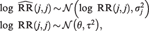
In a conventional meta-analysis, to summarize the different $\log (\widehat{\text{RR}}(j,j))$ , one would consider a standard random-effect model:

$$\begin{array}{l}\log \widehat{\text{RR}}(j,j)\sim \mathcal{N}\left(\log \text{RR}(j,j),{\sigma }_j^2\right)\\ \log \text{RR}(j,j)\sim \mathcal{N}\left(\theta ,{\tau }^2\right),\end{array}$$

for $j=1,\dots ,K$ , where θ, ${\tau }^2$ and ${\sigma }_j^2$ denote the summary effect, the between- and within-trial variance, respectively. This model can be equivalently expressed as:

$$\log \widehat{\text{RR}}(j,j)=\theta +{\alpha }_j+{\epsilon }_j$$

(6)

where the random-effect ${\alpha }_j\sim \mathcal{N}(0,{\tau }^2)$ expresses between-study heterogeneity, and the random error ${\epsilon }_j\sim \mathcal{N}(0,{\sigma }_j^2)$ reflects imprecision. Here, α_j and ${\epsilon }_j$ are commonly assumed to be independent. Based on this, the conventional I² statistic is defined as $I^2={\widehat{\tau }}^2/({\widehat{\tau }}^2+s^2)$ , where $s^2=\left\{{\displaystyle {\sum }_{j=1}^K{w}_j}(K-1)\right\}/\left\{{({\displaystyle {\sum }_{j=1}^K{w}_j})}^2-{\displaystyle {\sum }_{j=1}^K{w}_j^2}\right\}$ and $w_j=1/\{\widehat{\text{var(}}\mathrm{log }\widehat{\text{RR}}(j,j))\}$ , while $\widehat{\text{var}}\mathrm{(log }\widehat{\text{RR}}(j,j))$ and ${\widehat{\tau }}^2$ denote a consistent estimator of the variance of the unstandardized log relative risk estimate $\log \widehat{\text{RR}}(j,j)$ and the between-trial variance ${\tau }^2$ , respectively. The conventional I² statistic hence reflects the proportion of total variance explained by the presence of between-trial heterogeneity. ¹⁰

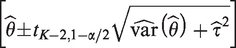
In standard random-effect meta-analysis, an alternative approach to represent between-trial heterogeneity is to establish a prediction interval which informs where the results of a future study can be expected with a pre-specified chance.^2,11 Higgins et al. proposed calculating the 100 $(1-\alpha )$ % prediction interval as:

$$\left[\widehat{\theta }\pm t_{K-2,1-\alpha /2}\sqrt{\widehat{\text{var}}\left(\widehat{\theta }\right)+{\widehat{\tau }}^2}\right]$$

where $\widehat{\theta }$ and $\widehat{\text{var}}\left(\widehat{\theta }\right)$ denote the estimate of the parameter θ in model (6) and its corresponding variance estimate, respectively. ² The use of different estimating methods for the between-trial variance ${\tau }^2$ can lead to different prediction intervals. Some of these suffer from under-coverage when the number of individual studies is low or when the amount of between-trial heterogeneity is small compared to the random error variances. ¹³ Alternatively, a Bayesian prediction interval for $\log \text{RR}(j,j)$ can also be computed. For this, one first randomly samples P values θ_i and ${\tau }_i^2$ (i = 1 to P) from their posterior distributions, then samples P values of $\log \text{RR}(j,j)$ from $\mathcal{N}({\theta }_i,{\tau }_i^2)$ . The resulting empirical distribution of $\log \text{RR}(j,j)$ can then be translated into a prediction interval.

Dismantling case-mix and beyond case-mix heterogeneity by I² statistics

In what follows, we propose a new approach that provides deeper insights into the between-trial variance ${\tau }^2$ in the conventional model (6). To achieve this, consider again the original relative risks $\text{RR}(j,j)$ and $\text{RR}(k,k)$ estimated in trial j and k, respectively, as well as the resulting $\text{RR}(j,k)$ when standardizing results of trial k over the case-mix of trial j:

$$\text{RR}(j,k)=\frac{{\displaystyle {\sum }_l\mathrm{Pr}}\left(Y=1|X=1,L=l,S=k\right)·\mathrm{Pr}\left(L=l|S=j\right)}{{\displaystyle {\sum }_l\mathrm{Pr}}\left(Y=1|X=0,L=l,S=k\right)·\mathrm{Pr}\left(L=l|S=j\right)}$$

From this, we see that the difference between $\text{RR}(j,j)$ and $\text{RR}(j,k)$ (or in more general cases, between the $\text{RR}(j,k)$ of the same population j) cannot be attributed to the difference in case-mix between trial j and k. This results from the fact that these relative risks share the same case-mix–related component $\mathrm{Pr}(L=l|S=j)$ in their structure. Therefore, the difference between $\text{RR}(j,j)$ and $\text{RR}(j,k)$ can only be explained by the beyond-case-mix difference reflected through the differential outcome generating mechanism $\mathrm{Pr}(Y=1|X=1,L=l,S)$ between trial j and trial k. By a similar reasoning, we see that $\text{RR}(j,k)$ and $\text{RR}(k,k)$ (or in more general cases, that the $\text{RR}(j,k)$ with the same index k) are heterogeneous due to the case-mix difference between trial j and k, as these relative risks share the same beyond-case-mix component, i.e. $\mathrm{Pr}(Y=1|X=1,L=l,S=k)$ , in their structure.

The above discussion hence makes clear that the presence of case-mix and beyond case-mix heterogeneity can be detected by looking at the variation among the $\text{RR}(j,k)$ which share the same value of j (for beyond-case-mix) or of k (for case-mix). In view of this, to measure the respective contribution of case-mix and beyond case-mix heterogeneity in the total discrepancy among trial results, one can consider the following random-effect model:

$$\log \widehat{\text{RR}}(j,k)=\theta +{\beta }_j+{\gamma }_k+{\epsilon }_{jk}$$

(7)

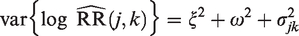
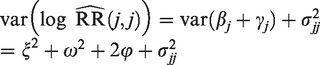
where ${\beta }_j\sim \mathcal{N}(0,{\xi }^2)$ and ${\gamma }_k\sim \mathcal{N}(0,{\omega }^2)$ denote two random-effect (RE) terms, and ${\epsilon }_{jk}\sim \mathcal{N}(0,{\sigma }_{jk}^2)$ continues to denote the residual random error. ${\xi }^2$ and ${\omega }^2$ are considered unknown, and ${\sigma }_{jk}^2$ is known for each j and k. With data from many trials, a correlation between β_j and γ_k can in principle be allowed, but we will for now assume these two random-effect terms to be mutually independent (and independent of the residual random terms ${\epsilon }_{jk}$ ). Correlated random effects will be subsequently discussed. The covariance matrix of the residual term ${\epsilon }_{jk}$ is left unstructured, as it is implied by the specific estimates $\widehat{\text{RR}}(j,k)$ . Under model (7) with independent random effects, the total variance of $\log \widehat{\text{RR}}(j,k)$ can be expressed as:

$$\text{var}\left\{\log \widehat{\text{RR}}(j,k)\right\}={\xi }^2+{\omega }^2+{\sigma }_{jk}^2$$

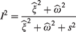
When j = k, we then have $\text{var}\left\{\log \widehat{\text{RR}}(j,j)\right\}={\xi }^2+{\omega }^2+{\sigma }_{jj}^2$ as a special case. Besides, note that if $\log \text{RR}(j,k)$ obeys model (7) for all j and k, the log relative risks $\log \text{RR}(j,j)$ will follow the standard random effect model (6). We thus have that ${\tau }^2={\xi }^2+{\omega }^2$ and ${\sigma }_j^2={\sigma }_{jj}^2$ , where ${\tau }^2$ and ${\sigma }_j^2$ are the between-trial variance and the random-error variance expressed in model (6), respectively. The standard I² statistic derived from model (6) can thus be equivalently expressed as:

$$I^2=\frac{{\widehat{\xi }}^2+{\widehat{\omega }}^2}{{\widehat{\xi }}^2+{\widehat{\omega }}^2+s^2}$$

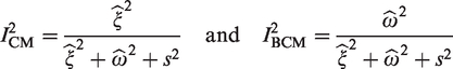
Reconsider now the different estimators $\log \widehat{\text{RR}}(j,k)$ of the same target population j with $k=1,\dots ,K$ . In model (7), these estimates share the same value for β_j, which implies that the variation (other than due to chance) among them is expressed by the random-effect term γ_k. The variance component ${\omega }^2$ thus reflects the amount of beyond case-mix heterogeneity among the K trials. Likewise, the random effect β_j models the variation among the different $\log \widehat{\text{RR}}(j,k)$ for the same trial conditions k. Its variance ( ${\xi }^2$ ) then reflects the amount of case-mix heterogeneity in the meta-analysis. The proportion of total variance explained by case-mix (CM) and beyond case-mix (BCM) heterogeneity can then be estimated as:

$$I_{\text{CM}}^2=\frac{{\widehat{\xi }}^2}{{\widehat{\xi }}^2+{\widehat{\omega }}^2+s^2}\text{and}{I}_{\text{BCM}}^2=\frac{{\widehat{\omega }}^2}{{\widehat{\xi }}^2+{\widehat{\omega }}^2+s^2}$$

respectively. Here, ${\widehat{\xi }}^2$ and ${\widehat{\omega }}^2$ denote consistent estimators of ${\xi }^2$ and ${\omega }^2$ (e.g. obtained by restricted maximum likelihood or Markov Chain Monte Carlo methods), respectively. The proposed statistics hence describe the extent to which each source of heterogeneity contributes to the total heterogeneity observed among trial results. For instance, a predominance of case-mix heterogeneity (indicated by a large $I_{\text{CM}}^2$ and a small $I_{\text{BCM}}^2$ ) suggests that the difference in marginal effect estimates among the trials might be mainly due to their differential case-mix, while the impact of beyond case-mix difference across trials is potentially trivial. When the random effects are independent, the sum of these two I² should be approximately equal to the one derived from a standard meta-analysis. In Appendix 2, we conduct a simulation study to illustrate these points.

Dismantling the two sources of heterogeneity by prediction intervals

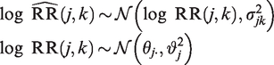
In what follows, we discuss the use of prediction intervals in decomposing case-mix and beyond case-mix heterogeneity. As a starting point, note that after case-mix standardization, the results $\widehat{\text{RR}}(j,k)$ obtained for the same population j can be summarized by a conventional meta-analysis of the form:

$$\begin{array}{l}\log \widehat{\text{RR}}(j,k)\sim \mathcal{N}\left(\log \text{RR}(j,k),{\sigma }_{jk}^2\right)\\ \log \text{RR}(j,k)\sim \mathcal{N}\left({\theta }_{j·},{\vartheta }_j^2\right)\end{array}$$

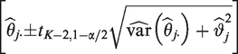
for $k=1,\dots ,K$ . In such a model, ${\theta }_{j·}$ represents the summary effect on the log relative risk scale with respect to population j, and ${\vartheta }_j^2$ expresses how much results from different trials vary even when considered for the same patient population j (e.g. as a result of beyond case-mix heterogeneity). When a frequentist approach is used to fit this model, an accompanying population j-specific prediction interval can then be established as:

$$\left[{\widehat{\theta }}_{j·}\pm t_{K-2,1-\alpha /2}\sqrt{\widehat{\text{var}}\left({\widehat{\theta }}_{j·}\right)+{\widehat{\vartheta }}_j^2}\right]$$

where ${\widehat{\theta }}_{j·}$ and ${\widehat{\vartheta }}_j^2$ denote the estimates of ${\theta }_{j·}$ and ${\vartheta }_j^2$ , respectively, while $\widehat{\text{var}}\left({\theta }_{j·}\right)$ denotes the variance estimate of ${\theta }_{j·}$ . Alternatively, one can use Bayesian approaches to fit the above model and to derive the corresponding prediction interval. The proposed prediction interval allows one to predict where the result of a new trial in population j can be expected with $(1-\alpha )100\%$ chance.

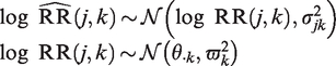
In a similar way, the results $\widehat{\text{RR}}(j,k)$ for the same population k can be summarized by a meta-analysis of the form:

$$\begin{array}{l}\log \widehat{\text{RR}}(j,k)\sim \mathcal{N}\left(\log \text{RR}(j,k),{\sigma }_{jk}^2\right)\\ \log \text{RR}(j,k)\sim \mathcal{N}\left({\theta }_{·k},{\varpi }_k^2\right)\end{array}$$

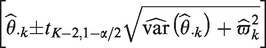
for $j=1,\dots ,K$ . Here, ${\varpi }_k^2$ expresses how much the result of trial k would vary if it were conducted in different patient populations with the same protocol k (e.g. as a result of case-mix heterogeneity). When a frequentist approach is used to fit this model, an accompanying protocol k-specific prediction interval can then be established as:

$$\left[{\widehat{\theta }}_{·k}\pm t_{K-2,1-\alpha /2}\sqrt{\widehat{\text{var}}\left({\widehat{\theta }}_{·k}\right)+{\widehat{\varpi }}_k^2}\right]$$

where ${\widehat{\theta }}_{·k}$ and ${\widehat{\varpi }}_k^2$ denote the estimates of ${\theta }_{·k}$ and ${\varpi }_k^2$ , respectively, while $\widehat{\text{var}}\left({\widehat{\theta }}_{·k}\right)$ denotes the variance estimate of ${\widehat{\theta }}_{·k}$ . Again, one can use Bayesian approaches to fit the above model and to derive the corresponding prediction interval. This interval allows one to predict where the result of trial k could be expected with a pre-specified chance, if it were conducted in different populations but according to the same protocol. In Appendix 3, we conduct a simulation study to illustrate these points.

I² statistic and prediction interval with correlated random effects

Case-mix and beyond case-mix heterogeneity may sometimes compensate each other and, in extreme cases, result in equal marginal effect sizes across the studies, thereby hiding these sources of heterogeneity. A numerical example of this is provided in the Online Supplementary Material file S5. Interestingly, the conventional model (6) will then have a between-trial variance of zero, which simply reflects the fact that the effect size does not vary across the studies. Such a finding may lead to a false-negative conclusion that trial results are statistically homogeneous and that the variation in case-mix and beyond case-mix across studies is trivial. Likewise, a conventional meta-regression of the form:

$$\log \widehat{\text{RR}}(j,j)=\alpha +\beta ·\widehat{\text{E}}(L|S=j)+{\delta }_j+{\epsilon }_j$$

$$\text{with }{\delta }_j\sim \mathcal{N}(0,{\vartheta }^2)\text{ and }{\epsilon }_j\sim \mathcal{N}(0,{\sigma }_j^2),$$

where $\alpha +\beta ·\text{E}(L|S=j)$ represents the treatment effect for population j, would find β = 0, thereby overlooking the potential importance of case mix heterogeneity on $\log \widehat{\text{RR}}(j,j)$ . The random-effect meta-analysis model (7) excludes this possibility of compensation via the assumption that the random effects are uncorrelated. In our proposed framework, such compensation may be taken into account by permitting a (negative) correlation between the two random effects β_j and γ_j in model (7), for then $({\beta }_j,{\gamma }_j)\prime$ follows a bivariate normal distribution with mean 0 and covariance matrix $\left(\begin{array}{cc}{\xi }^2& \phi \\ \phi & {\omega }^2\end{array}\right)$ . By assuming independence between a_j and b_k when $j\ne k$ , as well as between the two random effects and the residual error ${\epsilon }_{jj}$ , the total variance $\text{var}\left(\log \widehat{\text{RR}}(j,j)\right)$ can then be expressed as:

$$\begin{array}{l}\text{var}\left(\log \widehat{\text{RR}}(j,j)\right)=\text{var}({\beta }_j+{\gamma }_j)+{\sigma }_{jj}^2\\ ={\xi }^2+{\omega }^2+2\phi +{\sigma }_{jj}^2\end{array}$$

In the extreme case where ${\xi }^2={\omega }^2$ and $\phi =-{\xi }^2$ (i.e. $a_j=-b_j$ ), the between-trial variance $\text{var }({\beta }_j+{\gamma }_j)$ reduces to zero. This reflects complete compensation of case-mix and beyond case-mix heterogeneity across the studies.

Under the extended random-effect meta-analysis model with correlated random effects, one can then apply the I² statistics (with the denumerator additionally including $2\phi$ ) and the prediction intervals defined above to evaluate the two types of heterogeneity. However, due to the additional component $2\phi$ in $\text{var}\left(\log \widehat{\text{RR}}(j,j)\right)$ , we now define a third I² statistic:

$$I_{\text{Corr}}^2=\frac{2\widehat{\phi }}{{\widehat{\xi }}^2+{\widehat{\omega }}^2+2\widehat{\phi }+s^2}$$

where $\widehat{\phi }$ denotes a consistent estimator for the covariance $\phi$ of the two random effects. By construction, $I_{\text{Corr}}^2$ can take negative values, while $I_{\text{CM}}^2$ and $I_{\text{CM}}^2$ can exceed 100% if the two random effects are negatively associated. In Appendix 4, we further investigate the behaviors of I² statistics and prediction intervals in the correlated-random-effect model (7), with different levels of correlation between case-mix and beyond-case-mix heterogeneity. In practice, we recommend allowing for correlation between the two random effects in model (7), as it allows for more flexibility in the model considered.

Application to the INDANA meta-analysis

We apply the proposed approaches to reanalyze the data of INDANA, an individual patients data (IPD) meta-analysis comparing the risk of cardiovascular death of patients with high cardiovascular risk on an anti-hypertensive drug treatment (i.e. thiazide diurectics and/or $\beta -$ blocker) versus placebo or no intervention. ²⁸ The data were available for ten randomized studies with 53,271 patients (26,441 in the control arm). For this illustration, we focus on 5 baseline variables that were collected across all studies, namely age, gender, BMI, systolic blood pressure and smoking status. These variables were previously found to be prognostic for cardiovascular death. To avoid (strong) positivity violations, we assess the overlap of all trials in terms of the distribution of each outcome prognostic factor (Appendix 5). This shows that the ten trials are quite different in terms of the age distribution (i.e. some focused on a middle-aged population, while others considered an elderly population). For illustrative purposes, we here analyze the data of the trials conducted on an elderly population, namely the COOP, ²⁹ EWPHE, ³⁰ MRC2, ³¹ SHEP ³² and STOP ³³ trials. These trials are indexed as S = 1 to S = 5, respectively. The final analysis hence includes 12,309 patients (6,205 in the control arm), with 829 cardiovascular deaths. The baseline information of patients in each trial is summarized in Appendix 5.

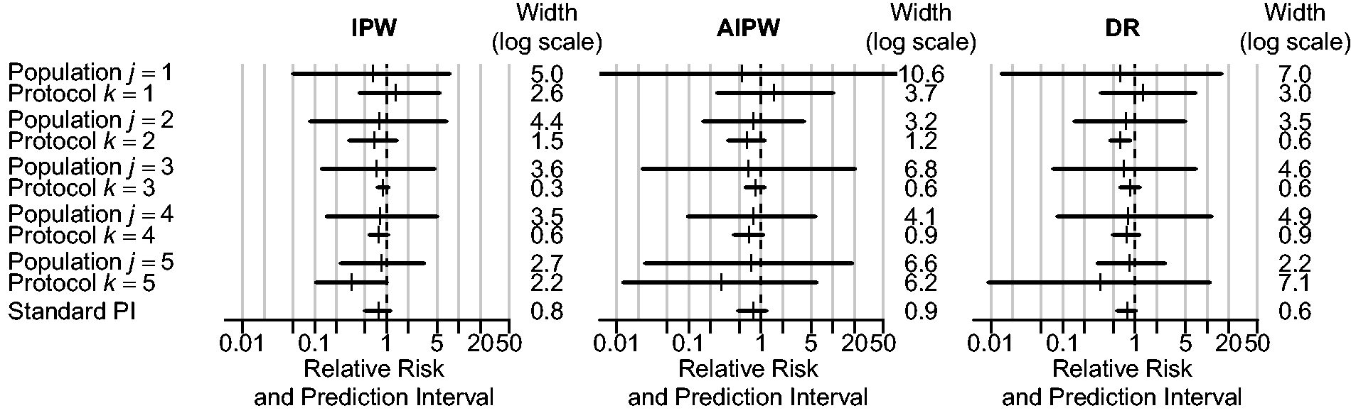
We standardize results of one trial over the case-mix of the other trials by using (i) the standard inverse probability weighting (IPW) approach, (ii) the doubly robust (DR) approach and (iii) the augmented inverse probability weighting (AIPW) approach. To derive the weights, we consider a multinomial logistic model of the form $\log \left\{\mathrm{Pr}(S=j|L)/\mathrm{Pr}(S=1|L)\right\}={\beta }_j\prime ·L$ , where $j=2\dots 5$ , L is the covariate vector including the value 1 and the main terms of the five considered baseline covariates, and β_j is the corresponding coefficient vector when S = j. The weights within each treatment arm of each trial are truncated by resetting the value of weights greater than the 95th percentile to the value of the 95th percentile (Figure 3), then stabilized as described in the second section. For the DR and AIPW approaches, when standardizing results of trial k over the case-mix of trial j, we consider a logistic outcome model of the form $\text{logit }\mathrm{Pr}(Y=1|X=x,L,S=k)={\gamma }_k\prime ·A$ where $A={\left(\begin{array}{ccc}1& x& L\end{array}\right)}^t$ , with L here denoting the main terms of the five considered baseline covariates, and γ_k is the corresponding coefficient vector when S = k. This model is fitted by weighting each patient i treated with X = x in trial j by the weight stabilized and truncated as described above. Parametric bootstrap is used to derive the covariance matrix of the standardized relative risks. As the overall missing data rate was low ( $\sim 2$ %), we consider a complete-case analysis.

In what follows, we fit model (7) with and without correlated random effects to summarize the standardized relative risks. The procedure is fully Bayesian and is based on Markov Chain Monte Carlo (MCMC) simulation. We consider weakly informative, independent prior distributions for the unknown parameters θ, ${\xi }^2,{\omega }^2$ and ρ (where $\rho =\phi /(\xi ·\omega )$ is only available in model (7) with correlated random effects). The prior for θ is the normal distribution $\mathcal{N}(0,1000)$ , for ξ and ω it is the uniform distribution U(0, 100), and for ρ it is a normal distribution $\mathcal{N}({\mu }_{\rho },{\sigma }_{\rho }^2)$ (where ${\mu }_{\rho }\sim U(-1,1)$ and ${\sigma }_{\rho }\sim \Gamma (1.5,{10}^{-4})$ ), truncated at –1 and 1. We assume that the residual covariance matrix is known a priori. To derive $I_{CM}^2,I_{\mathit{BCM}}^2$ and $I_{\mathit{Corr}}^2$ , we randomly sample 10 000 values of ${\xi }^2,{\omega }^2$ and ρ from the corresponding posterior distributions, then calculate $I_{CM}^2,I_{\mathit{BCM}}^2$ and $I_{\mathit{Corr}}^2$ as proposed above. The empirical (posterior) distribution of these I² is then summarized by the posterior mean and the corresponding 95% credible interval.

For a comparison, we also fit the standard random-effect model (i.e., model (6)) to summarize the unstandardized relative risks. In this model, the prior for θ is the normal distribution $\mathcal{N}(0,1000)$ and for τ it is the uniform distribution U(0, 100). These prior distributions are independent We also assume that the variances ${\sigma }_{jk}^2$ of the residual errors ϵ_jk ( $j,k=1,\dots ,5$ ) are known a priori. To derive the population j- (or protocol k-) specific prediction intervals, we first summarize the standardized relative risks $\log \widehat{\text{RR}}(j,k)$ that share the same value of j (or of k) by using model (6) with the above numerical setup. We then randomly sample 10 000 values of ${\theta }_{j.}$ and of ${\vartheta }_j^2$ (or of ${\theta }_{.k}$ and of ${\varpi }_k^2$ ) from the corresponding posterior distributions, then generate 10 000 values of $\log \text{RR}(j,k)$ for k = 1 to 5 (or for j = 1 to 5) from the distribution $\mathcal{N}({\theta }_{j.},{\vartheta }_j^2)$ (or $\mathcal{N}({\theta }_{.k},{\varpi }_k^2)$ ). The population j- (or protocol k-) specific prediction interval is then computed based on the 2.5% and 97.5% quantiles of the empirical distribution of $\log \text{RR}(j,k)$ . We run MCMC for all models in R (version 3.4.4) by using the package rjags, with 2 chains and 50 000 burn-in iterations followed by 500 000 updates.

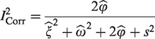
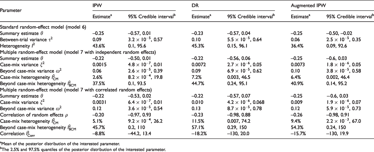
As can be seen in Table 1, the conventional I² statistic (36.5% to 44.4%) suggests that there is a moderate amount of statistical heterogeneity in the meta-analysis. The proposed I² statistics further indicate that this heterogeneity is mostly due to beyond case-mix reasons. The proposed prediction intervals also suggest that beyond case-mix tends to be more important than case-mix in explaining the total heterogeneity (Figure 2). These findings were consistent regardless of the approach being used. In practice, other choices of priors for the parameters should also be considered to assess the sensitivity of the findings.

Table 1.

INDANA meta-analysis: results of different random-effect models.

Parameter	IPW		DR		Augmented IPW
	Estimate a	95% Credible interval b	Estimate a	95% Credible interval b	Estimate a	95% Credible interval b
Standard random-effect model (model 6)
Summary estimate θ	–0.25	–0.57, 0.01	–0.23	–0.57, 0.04	–0.25	–0.50, –0.02
Between-trial variance ${\tau }^2$	0.09	$3.2\times {10}^{-5}$ , 0.57	0.10	$5.5\times {10}^{-5}$ , 0.64	0.06	$2.5\times {10}^{-5}$ , 0.35
Heterogeneity I2	43.6%	0.1, 95.6	45.3%	0.15, 96.1	36.4%	0.09, 92.6
Multiple random-effect model (model 7 with independent random effects)
Summary estimate θ	–0.22	–0.50, 0.01	–0.22	–0.56, 0.06	–0.25	–0.6, 0.03
Case-mix variance ${\xi }^2$	0.0015	$4.8\times {10}^{-7}$ , 0.01	0.0072	$2.7\times {10}^{-6}$ , 0.05	0.0073	$1.8\times {10}^{-6}$ , 0.05
Beyond case-mix variance ${\omega }^2$	0.06	$2.6\times {10}^{-5}$ , 0.39	0.09	$6.9\times {10}^{-5}$ , 0.62	0.10	$3.8\times {10}^{-5}$ , 0.58
Case-mix heterogeneity $I_{\text{CM}}^2$	2.6%	$8.2\times {10}^{-4}$ , 19.8	7.2%	0.003, 46.5	6.4%	0.002, 46.4
Beyond case-mix heterogeneity $I_{\text{BCM}}^2$	37.5%	0.1, 93.5	44.7%	0.24, 95.1	40.9%	0.14, 95.2
Multiple random-effect model (model 7 with correlated random effects)
Summary estimate θ	–0.22	–0.53, 0.02	–0.22	–0.57, 0.07	–0.25	−0.6, 0.03
Case-mix variance ${\xi }^2$	0.0031	$6.4\times {10}^{-7}$ , 0.01	0.010	$4.2\times {10}^{-6}$ , 0.068	0.009	$1.9\times {10}^{-6}$ , 0.07
Beyond case-mix variance ${\omega }^2$	0.12	$3.6\times {10}^{-5}$ , 0.54	0.13	$8.7\times {10}^{-5}$ , 0.78	0.12	$5.9\times {10}^{-5}$ , 0.73
Correlation of random effects ρ	–0.20	–0.97, 0.93	–0.23	–0.98, 0.88	–0.26	–0.98, 0.91
Case-mix heterogeneity $I_{\text{CM}}^2$	5.1%	$9.2\times {10}^{-4}$ , 26.2	11.5%	0.007, 74.2	9.4%	$2.2\times {10}^{-3}$ , 67.0
Beyond case-mix heterogeneity $I_{\text{BCM}}^2$	45.7%	0.2, 110	57.1%	0.29, 150	54.3%	0.24, 150
Correlation $I_{\text{Corr}}^2$	–8.8%	–44.2, 13.4	–18.2%	–130, 20.0	–15.7%	–130, 19.9

^aMean of the posterior distribution of the interested parameter.

^bThe 2.5% and 97.5% quantiles of the posterior distribution of the interested parameter.

Figure 2.

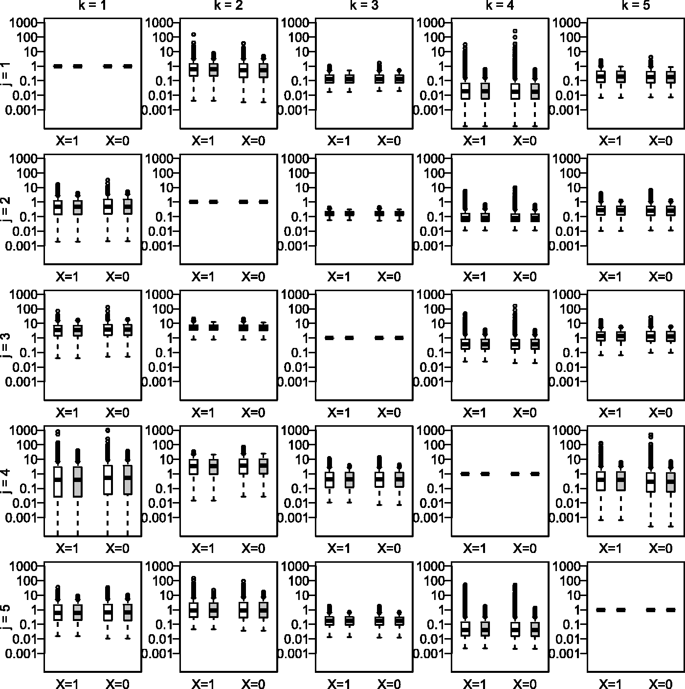
INDANA meta-analysis: population-specific and protocol-specific 95% prediction intervals. Population-specific prediction interval are derived after summarizing $\widehat{\text{RR}}(j,k)$ with j fixed and $k=1\dots 5$ . Protocol-specific prediction intervals are derived after summarizing $\widehat{\text{RR}}(j,k)$ with k fixed and $j=1\dots 5$ . The standard prediction interval is the 95% prediction interval obtained after a standard random-effects meta-analysis. The population-j-specific prediction interval predicts where the result of a new trial conducted in population j can be expected with 95% chance. The protocol-k-specific prediction interval predicts where the result of the trial k can be expected with 95% chance, if this trial follows the same protocol but is being conducted in a new population.

Figure 3.

INDANA meta-analysis: distribution of the weights $\widehat{\mathrm{Pr}}(S=j|L)/\widehat{\mathrm{Pr}}(S=k|L)$ before (white) and after (grey) 95th percentile truncation. The first two boxplots are for the treated group (X = 1), and the last two are for the control group (X = 0).

Figure 4.

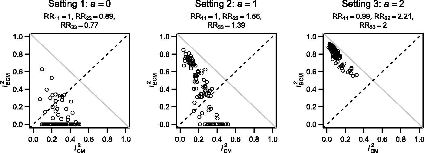
Case-mix and beyond case-mix heterogeneity captured by the two I² statistics across the 3 settings. The closer the points are to the grey line $I_{CM}^2+I_{\mathit{BCM}}^2=1$ , the smaller the value of s² is compared to ${\xi }^2$ and ${\omega }^2$ .

Discussion

Case-mix variation across eligible studies affects many meta-analyses. It often contributes significantly to the overall statistical inconsistency observed among trial results. In this paper, we discuss the use of two conventional statistics, i.e. the I² statistic and the prediction interval, to disentangle the impact of case-mix and beyond case-mix heterogeneity on the final summary estimate. In practice, these approaches can be used to support the standard heterogeneity assessment conducted in conventional meta-analyses. In particular, the proposed prediction intervals can be used to appreciate where the result from a new trial may be expected when it is conducted on the same patient population, or following the same protocol. Case-mix and beyond case-mix may sometimes compensate each other. In extreme cases, this may result in approximately equal marginal effect estimates, thereby rendering standard heterogeneity assessments misleading (as the between-trial variance will then equal zero in the conventional meta-analysis). In such situation, the proposed approaches give a better reflection of the degree of heterogeneity and shed insightful light on possible compensation of different sources of heterogeneity.

The major impediment to the proposed approaches is the need for access to the individual patient data needed for estimating the case-mix standardized treatment effects. In future work, we will therefore generalize these approaches to partially aggregated-data meta-analysis. Another challenge arises from the possible risk of model misspecification when estimating the probability $\mathrm{Pr}(S=j|L)$ . In practice, this estimation is best based on a flexible propensity score model that incorporates many covariates as well as relatively many possible covariate-covariate interactions. If stepwise model building approaches are adopted, we recommend screening at a relatively large significance level (e.g., 15 or 20%) to ensure a sufficient adjustment for case-mix.

To summarize, we conclude that case-mix standardization can bring several advantages to the standard heterogeneity assessment conducted in meta-analyses. This approach, therefore, should be further evaluated to increase its applicability in meta-analysis practice.

Software

The simulated data and computing codes required to replicate the results reported in this paper are available in the Online Supplemental Material file. We are not allowed to distribute the INDANA IPD meta-analysis data, and access should be directly requested to the INDANA steering group.

Supplemental Material

sj-pdf-1-rmm-10.1177_2632084320957207 - Supplemental material for Assessing the impact of case-mix heterogeneity in individual participant data meta-analysis: Novel use of I² statistic and prediction interval

Supplemental material, sj-pdf-1-rmm-10.1177_2632084320957207 for Assessing the impact of case-mix heterogeneity in individual participant data meta-analysis: Novel use of I² statistic and prediction interval by Tat-Thang Vo, Raphaël Porcher and Stijn Vansteelandt in Research Methods in Medicine & Health Sciences

Supplemental Material

sj-pdf-2-rmm-10.1177_2632084320957207 - Supplemental material for Assessing the impact of case-mix heterogeneity in individual participant data meta-analysis: Novel use of I² statistic and prediction interval

Supplemental material, sj-pdf-2-rmm-10.1177_2632084320957207 for Assessing the impact of case-mix heterogeneity in individual participant data meta-analysis: Novel use of I² statistic and prediction interval by Tat-Thang Vo, Raphaël Porcher and Stijn Vansteelandt in Research Methods in Medicine & Health Sciences