Sage Journals: Discover world-class research

Abstract

Unplanned dilution in underground mining is detrimental to the business, as imprecise dilution factors may impair production forecasts for existing operations or the economic evaluation and viability of brownfield expansions and greenfield projects. While high prediction accuracy of over 90% has been achieved using machine learning algorithms, particularly artificial neural networks (ANNs), the studies mostly predicted the overall dilution of stopes or included performance-subjective determinants, such as drill and blast factors. These factors compromise the models’ reproducibility for extensional application to cover new mining projects that do not have historical drill and blast input. To address this, the study explores gene expression programming (GEP) and ANN with backpropagation (BPNN) to predict dilution on a per-stope granularity based on geotechnical and design data. A 138-stope sample from a sublevel open stoping gold mine operation in Western Australia was used to generate predictive models. Model and infield results showed that the GEP model performed better, with a coefficient of determination, R², of 0.740 with a root mean square error (RMSE) of 0.361 compared to BPNN's 0.681 and 0.409, respectively. Accordingly, the GEP model is recommended for dilution prediction for mine planning and production scheduling at the prescribed level of accuracy.

Keywords

machine learning gene expression programming BP-neural networks dilution prediction open stoping artificial neural networks

Preliminaries and motivation

Predictive machine learning (ML) algorithms are increasingly being deployed to infer underground mining performance metrics such as mining dilution, improving the robustness of performance forecasts and enabling the upfront establishment of appropriate mitigatory controls (Nanda, 2020; Chimunhu et al., 2024b). Various underground mining methods exist, with the open stoping method being the most commonly used, particularly for narrow to medium-width orebodies. The method is preferred for its simplicity in execution and retreat methodology, which minimises personnel exposure to mined voids. Input assumptions such as mining dilution and recovery are essential in estimating the mining efficiency of planned mining blocks, called stopes. In particular, dilution accounts for the additional percentage of subeconomic or waste material mined in the course of extraction of the planned stope and is dependent, to a large extent, on rockmass quality, stope geometry and design, amongst other factors (Henning, 2007; Henning and Mitri, 2008; Mathews et al., 1980; Sutton, 1998). Figure 1 provides a simplistic overview of planned and unplanned dilution for a stope in open stope mining. The mining dilution factor is one of the underlying key input assumptions used in generating production schedules that forecast quantities (tonnes) and quality (grades) of metal to be mined per period (usually monthly) over the remaining life of the business. The schedules’ production forecasts are then used to project the business cash flows and assess the sustainability of operating projects or the economic viability of brownfield expansions (i.e. near-mine extensions where geological/geotechnical continuity is not confirmed but may be assumed based on their proximity to existing areas) and greenfield projects (i.e. new mining projects planned and mostly rely on transferable methodologies established elsewhere to establish suitable project-specific assumptions).

Figure 1.

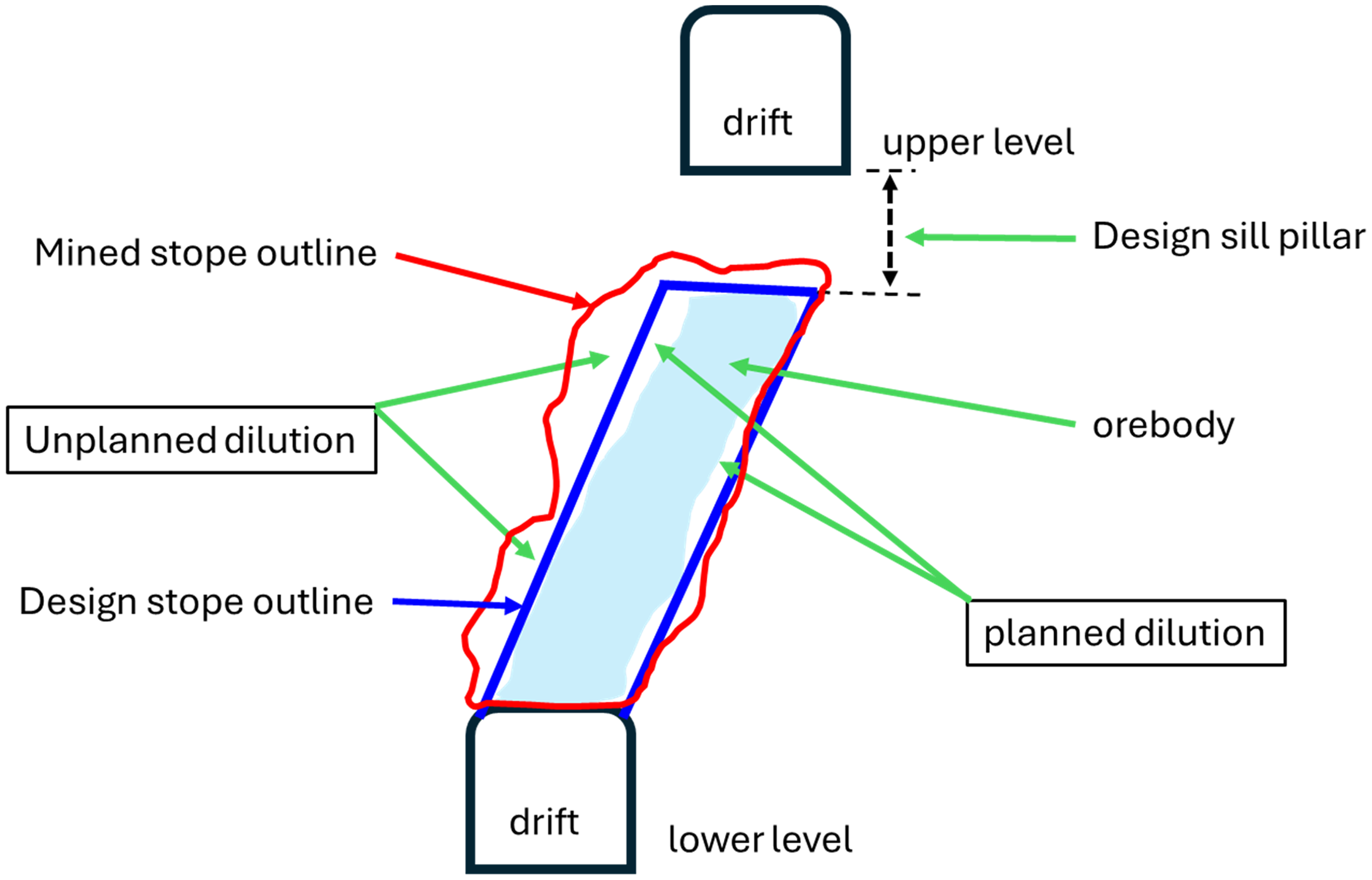
Planned and unplanned mining dilution in open stope mining.

Evidently, a robust dilution estimate is crucial in production forecasting as an underestimate/overestimate affects projected production volumes with serious ramifications to the project's financial performance (Planeta et al., 1990). Yet, despite this glaring fundamental, the common practice in mine planning uses a flat dilution factor for all stopes, in existing mine areas or brownfields and greenfield extensions. The adopted flat factor is usually derived from the historical stope performance data on prior mined stopes, whose performance may not adequately reflect future performance due to differences in the transitional degree of interactions amongst the causative factors as ground conditions and design attributes evolve (Chimunhu et al., 2024a). As a result, opportunities to implement targeted controls on potential high-dilution stopes or optimise production schedules based on a granular prediction of individual stope performance are lost. Further, as production schedules are usually developed years ahead of actual mining to inform high-level economic viability and business sustainability and related decisions, it is prudent that robust dilution factors are established based on stope-specific data available at the early stages of stope design and schedule generation. While prefeasibility data may be limited and crude, its application for dilution prediction provides fundamental insights on the phenomenon, unbiased by human-induced factors such as drill and blast performance, enhancing the generalisation of findings and transferability of concepts to new mining projects.

The stope's geotechnical properties, such as the rock quality designation (RQD), modified stability number ( $N^{'}$ ), rockmass rating (RMR) and Q-rating (Q and Q′), which generally measure the quality of the rockmass, have been found to have an indirect correlation with dilution (Clark, 1998; Mathews et al., 1980; Potvin, 1989), with parameters such as rock Joint spacing (Js), Joint alteration (Ja), Joint water (Jw), Joint roughness (Jr) and stress reduction factor (SRF) moderating the rockmass classification according to the relationship expressed in equation (1) (Henning and Mitri, 2008; Hughes, 2011; Sutton, 1998; Urli, 2015):

Q = \frac{R Q D}{J_{n}} \times \frac{J_{r}}{J_{a}} \times \frac{J_{w}}{S R F},

(1)where J_w/ SRF represents the stress factor, in the absence of which, equation (1) then measures a moderated but still effective value of Q, known as Q-prime (Q′). Extant literature on dilution and overbreak in both mining and tunnelling has shown that rockmass with higher quality (

N^{'}

, Q, RQD) classification/rating are generally less susceptible to dilution and vice versa (Mathews et al., 1980; Papaioanou and Suorineni, 2016; Sutton, 1998; Suorineni, 2010). Further, stope dimensions of width, length, height and aspect ratio (width to height ratio) have also been proven to influence dilution through the effects of hydraulic radius (HR) on hanging wall stability (Sutton, 1998; Suorineni, 2010; Szmigiel et al., 2024). Long and wide spans are more prone to hanging failure (dilution) than short and narrow spans, while shallow dipping stopes are more prone to hanging wall failure than steep stopes due to the increased gravitational effect on the hanging wall (Abdellah Wael et al., 2020; Hefni et al., 2020; Henning, 2007; Hughes, 2011). Additionally, drill and blast human-induced mining errors such as drill hole deviation and excessive explosive charge density potentially increase the risk of premature hanging wall failure, resulting in excessive dilution. Furthermore, the degree of weathering has also been noted to influence dilution by compromising the rock's strength and, therefore, increasing its susceptibility to failure (Forster et al., 2007). While the list of causative factors is not exhaustive, several studies have also shown that sufficiently high levels of prediction can still be achieved with the right combination of a few critical factors.

The Mathews stability graph, proposed by Mathews (Mathews et al., 1980), and later modified by Potvin (Potvin, 1989) and other scholars, is one of the most widely used empirical methods for predicting hanging wall stability and dilution in underground mining. The method predicts hanging wall stability through graphical delineation of zones of stability and instability based on the modified stability number (N′) and hydraulic radius (HR) of a mined void (Sutton, 1998; Suorineni, 2010). The relationship between the modified stability number, N′ and $Q^{'}$ is expressed as follows (Papaioanou and Suorineni, 2016):

N^{'} = Q^{'} \times A \times B \times C,

(2)where Q′ is the rock quality index and A, B and C are the stress reduction, joint orientation and gravity adjustment factors, respectively. The hydraulic radius (HR) represents the dimensions and shape of the stope, i.e. the stope design/geometry, and is mathematically expressed as follows (Papaioanou and Suorineni, 2016):

H R = (w \times h) / 2 (w + h),

(3)where w represents the length of the exposed stope and h represents the stope height. Despite its notable successes in application, the stability graph's limitations in addressing complex stope geometries and its subjectivity in defining the stability graph zones, amongst other factors, necessitated improvements that eventually culminated in the introduction of the equivalent linear overbreak slough (ELOS) graph concept by Clark (1998) to simplify the irregular overcut depth of the hanging wall (dilution) into a linear average for ease of quantification. However, it is worth noting that while the ELOS measurement of dilution is widely used and accepted, it is sensitive to orebody widths, and therefore, its application and interpretation require consideration of that fact (Suorineni, 2010). As ML methods penetrated deeper into facets of underground mining, their application extended to dilution prediction with supervised decision tree-based models, such as the random forest (RF) (Chongchong et al., 2018) and artificial neural networks (ANNs) (Mottahedi et al., 2018; Zhao and Jia’an, 2020), producing remarkable prediction results. In particular, a recent dilution prediction study by Jorquera et al. (2023) based on 752 cases from open stoping underground mines in Chile, Argentina, and Brazil reported an impressive prediction accuracy of 94%. However, the dilution factor was categorised into five classes, focusing on a dilution bandwidth of 0–20%, with dilution above 20% as one large outlier category. Further, as the RF model utilises categorical classification in its prediction, its granularity and accuracy are largely influenced by the bandwidth of categories rather than each stope's unique and distinctive properties, rendering it less effective for dilution prediction on a per-stope basis. Therefore, ML models, such as ANN, that can handle continuous input and output data variables are preferred for dilution prediction on a per-stope fidelity. Indeed, some high-accuracy ANN model prediction results were noted from related early studies conducted on a tunnelling project in Gumi, South Korea, by Jang and Topal (2013). The authors reported a dilution prediction accuracy of over 94.5% based on 49 sets of RMR ratings from a tunnelling project. While the results were significant, they did not reflect the typical underground mining production environment, as was proved a few years later when the authors extended their original study to cover the long hole open stoping (LHOS) underground operations and reported a 22.6% lower prediction accuracy of 71.9% (Jang et al., 2015). Additionally, the authors included human-influenced factors such as drill and blast performance. Such factors included blasting data such as powder factor, drill hole deviation and burden and spacing, which not only introduced human error bias but also meant the model's reproducibility for extensional application to cover brownfield expansions or new mining projects that do not have historical drill and blast input data was undermined. As a result, its generalisation capabilities to cover brownfield extensions and greenfield projects were curtailed. Similarly, Zhao and Jia’an (2020) also used ANN with backpropagation for dilution prediction based on 120 sets of data from several mines, which included 20 synthetic data sets and reported a prediction accuracy of 97.6%. However, the model also used drill and blast data inputs of borehole deviation and charge density. Further, the mining methods from which the 100-set data was obtained were not disclosed, rendering it difficult to relate to open stoping operations. A summary of these studies is presented in Table 1. Clearly, the ANN model can achieve higher prediction accuracy (Table 1) than tree-based models such as RF. However, while ANN models may offer higher accuracy, they function as black boxes, making it difficult to interpret the influence of individual parameters. Tree-based models, on the other hand, provide insight into the contribution of each parameter.

Table 1.

Summary of key studies on dilution prediction in underground mining and tunnelling.

Study	Input variables	Mining type	Method(s)	Test accuracy
Jang and Topal (2013)	UCS, RQD, Js, Jo, Ja, Jw, RMR	Tunnelling	ANN	94.5
Jang et al. (2015)	Q, width to height ratio, D&B	UGM (OS)	ANN	71.9
Chongchong et al. (2018)	RQD, Js, Jo, Ja, Jw, A, B, C, height, dip, strike dilution graph factor, stress factors	UGM (OS)	RF	87.3
Mottahedi et al. (2018)	RMR, D&B	Tunnelling (CM)	Fuzzy	97
Zhao and Jia’an (2020)	N, HR, D&B	UGM	ANN	97.6
Jorquera et al. (2023)	Q, A, B, C, height, width, length, dip	UGM (OS)	RF	94.2
Current study	Dip, stope size, HR, N'	UGM (OS)	GEP &ANN

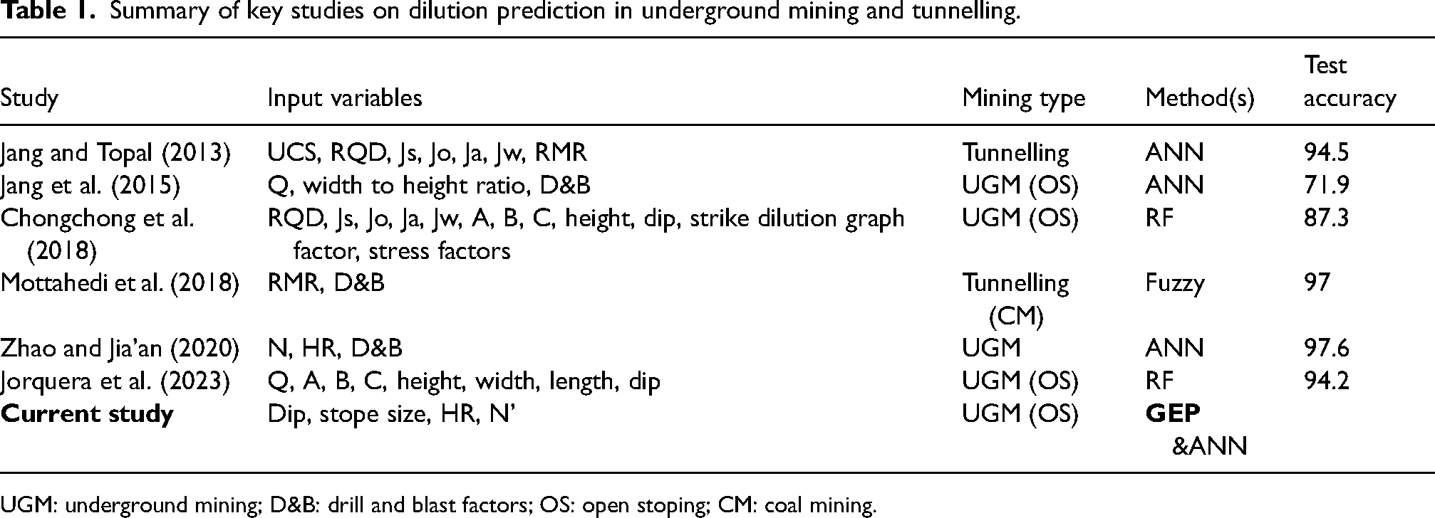
UGM: underground mining; D&B: drill and blast factors; OS: open stoping; CM: coal mining.

Further, the studies also reveal that a high prediction accuracy of over 90% observed in ANN models is achieved mostly in the tunnelling environment or when additional factors, such as the human-influenced drill and blast performance, are considered.

However, Jang et al. (2016) established that rock quality, stope width, mining depth and the horizontal to vertical stress ratio were key dilution causative factors, with drill and blast factors ranked as secondary causatives in their investigatory study on the relative importance of 10 dilution causative factors. Further, these findings were also complimented by Chongchong et al. (2018), who concluded that the stope design method, RQD, stope height, dip, strike and joints data were primary drivers of dilution in underground mining based on 13 influencing variables analysed from a sample of 115 hanging wall cases for sub-level open stoping (SLOS) operations using the RF algorithm. A recent study on dilution for open stoping operations by Cadenillas (2023) also confirmed that stope height, length, width, hydraulic radius and dip angle significantly influenced dilution based on 29 causative variables for underground mining. This suggests that while there are numerous causative variables, variables related to rockmass quality and stope geometry are principal predictors that significantly influence prediction accuracy. Further, human-influenced factors such as drill and blast performance have improved prediction accuracy, albeit as secondary determinants. Therefore, the omission of such in other studies that still managed to achieve prediction accuracy of over 70% strongly suggests their influence is minimal, considering the bias they potentially introduce arising from subjectivity on human performance and potential human errors. This perspective is supported by Urli (2015), who asserts that rockmass quality (as measured by the modified stability number, N′) and stope spans (HR) are chief causes of dilution and proposes ore-skin design options, which minimise hanging wall disturbance or dilution by not extending blast holes to hanging wall contact. Further, Mateo et al. (2024) also proposed and successfully demonstrated the variability of drill- and blast-related dilution through the application of presplitting blasting techniques at Pique mine in the El Oro province of Ecuador, suggesting that the influence of drill and blast factors on dilution can be considered and handled at a localised scale based on site-specific mining standards and experience. On a similar note, Delentas et al. (2021) argue that optimising the design features of the stopes at the early design stage (stope geometry) is one of the most effective control mechanisms for dilution in underground mining based on the results of their study on stability conditions and dilution in open stoping operations. Such initiatives include optimal placement of drives relative to the reef to minimise footwall trenching dilution when it comes to stope production, control of production drill hole deviation using drill-mounted azimuth aligners and a plethora of other drill and blast controls that are being made possible by an increasing realisation of the possibility of ML augmented capabilities in underground mining (Chimunhu et al., 2024b). As such, drill- and blast-induced variations are expected to be small to moderate, well within reach of the capacity of modern mining standards.

Soft computing methods have also been used to predict dilution in related tunnelling studies, with a prediction accuracy of over 84% reported (Mottahedi et al., 2018). However, these methods have not been sufficiently extended to cover underground mining operations such as open stoping. In the past decade, evolutionary ML models such as genetic algorithms (GAs) have shown a continued and stable application in prediction and forecasting studies, as ANN models are usually not the first models of choice due to their black-box nature in their prediction architecture. In particular, gene expression programming (GEP), a sibling of genetic programming algorithms inspired by the Darwinian evolutionary theory of ‘Survival of the Fittest’ (Roohollah Shirani et al., 2017; Shirani et al., 2024), is increasingly being used to develop mathematical predictive models. The model was first introduced by Ferreira et al. (2002), leveraging the merits and overcoming the limitations of the pioneering works of Koza (1994) and Sampson (1976). In its simplest form, the GEP model, like the GA, utilises a randomly generated sample population (chromosomes) as the initial population. This population is then improved multiple times (evolution) through activation by a group of genetic operators (mutation, crossover, reproduction, etc.). The dominant characteristic genes of the surviving population then represent the model's solution, encoded in strings called chromosomes. The solution is expressed in a branch-like structure linked by genetic operators that describe the multiple relationships between the leaves. In its mathematical presentation, the model's ability to generate clear and structured mathematical representations of complex systems and phenomena through its mutational architecture offers increased visibility to underlying relations for modelling complicated relationships often handled by neural networks in a black-box architecture. Further, its successful application in related mining studies, such as the prediction of rockbursts (Shirani Faradonbeh et al., 2022; Shirani et al., 2024), blast-induced ground vibrations (Faradonbeh and Monjezi, 2017; Shirani Faradonbeh et al., 2016) and more recently, hanging wall stability in underground mining (Amirkiyaei et al., 2023; Jalilian et al., 2024), lends its credibility in offering potential solutions to extensional studies such as overbreak prediction (dilution) in underground mining as proposed in this study.

This study aims to establish a dilution prediction model for individual stopes based on geological/geotechnical and geometrical (design) attributes and generate a mathematical equation of the model to facilitate the optimisation of production schedules through granular predictions on stope performance. The study also aims to establish a dilution prediction model that is not influenced by human performance factors such as drill and blast performance and, therefore, is generalisable for extensional applications in open stoping operations at the strategic level of detail. When that is achieved, the novel contribution of this study to existing literature emanates from using a unique set of data available at the early stages of mine planning to predict dilution on a per-stope basis. Further, the study's significance lies in its pioneering incubation of a GEP-based methodology for dilution prediction in underground open stope mining operations, where currently, to the authors’ knowledge, no known studies have explored its application. While the crudeness of the input data at the early stages of mine planning and production schedule generation points to potential challenges in achieving high prediction accuracy, this study seeks to harness the merits of the increasing ability to use reduced data inputs and still generate more insights, utilising the computing power of modern-day computing systems coupled with emerging ML applications as proposed by Chimunhu et al. (2022, 2024c) and Buaba (2023). While the deliberate omission of drill and blast input may result in a lower prediction than when included, the prediction is not impaired by the subjectivity of human performance that comes with its inclusion. Further, if modelling and prediction with fewer data achieve a considerably high prediction accuracy, this may save on the additional time and costs that would have been required to generate more data and, more importantly, will likely bring production schedules and cash flows forward with an earlier start in production.

In a nutshell, the chronological progression of studies on mining dilution largely shows an increasing inclination to include drill and blast factors to improve prediction accuracy. However, including drill and blast factors requires that a reasonably large number of stopes are mined first to create the relevant database. As such, the results will be limited in application scope, particularly when planning for brownfields extension or greenfield projects where no drill and blast and related databases exist. Few studies that have not considered drill- and blast-related factors continue to face challenges in achieving relatively high prediction, particularly for prediction on a per-stope basis. This study leverages literature to explore different input variables, riding on the merits of emerging ML applications such as gene expression programming, which has not been used extensively in previous related studies.

Data collection and preparation

Parametric and geotechnical data for 167 stopes was collected from an anonymised multireef narrow to medium-width orebody open stope mining operation in Western Australia. Parametric data focused on stope size (T), dip (A) and dimensions to calculate hydraulic radius, HR, while geotechnical data comprised additional random checks on rock quality measures to verify stope stability numbers (N) acquired from the geotechnical database. The equivalent linear overbreak slough (ELOS) measurement method was used to convert measured dilution values from percentage form to metres for a linearised transformation of the values to improve dimensional consistency with other variables. The dilution proxy, equivalent ELOS, was back-calculated from percentage form and converted to ELOS classification system as per equation (4):

ELOS = \frac{V_{s}}{A_{s}}

(4)where V_s is the volume of the overbreak slough and A_s is the stope's surface area.

This transformation was essential for comparing dilution on stopes with different widths, as percentage dilution factors do not reflect the comparative magnitude of hanging wall overbreak (dilution) when assessing stopes with different widths. The resultant ELOS equivalent dilution proxy will later be reconverted back to percentage form for production scheduling purposes. ELOS values above 3 m were discarded as such magnitude of overbreak is generally regarded as a failure criterion and not overbreak (Brady et al., 2005). A desurvey of the mine's exploration drill hole database was conducted to randomly check some of the drill hole intercepts on the sample stopes and use the borehole data to check the core samples and logged geological and geotechnical data for any obvious discrepancies. Further, a correlation matrix was used to assess any interference amongst the variables that could lead to redundancies or poor model calibration and performance (Figure 2).

Figure 2.

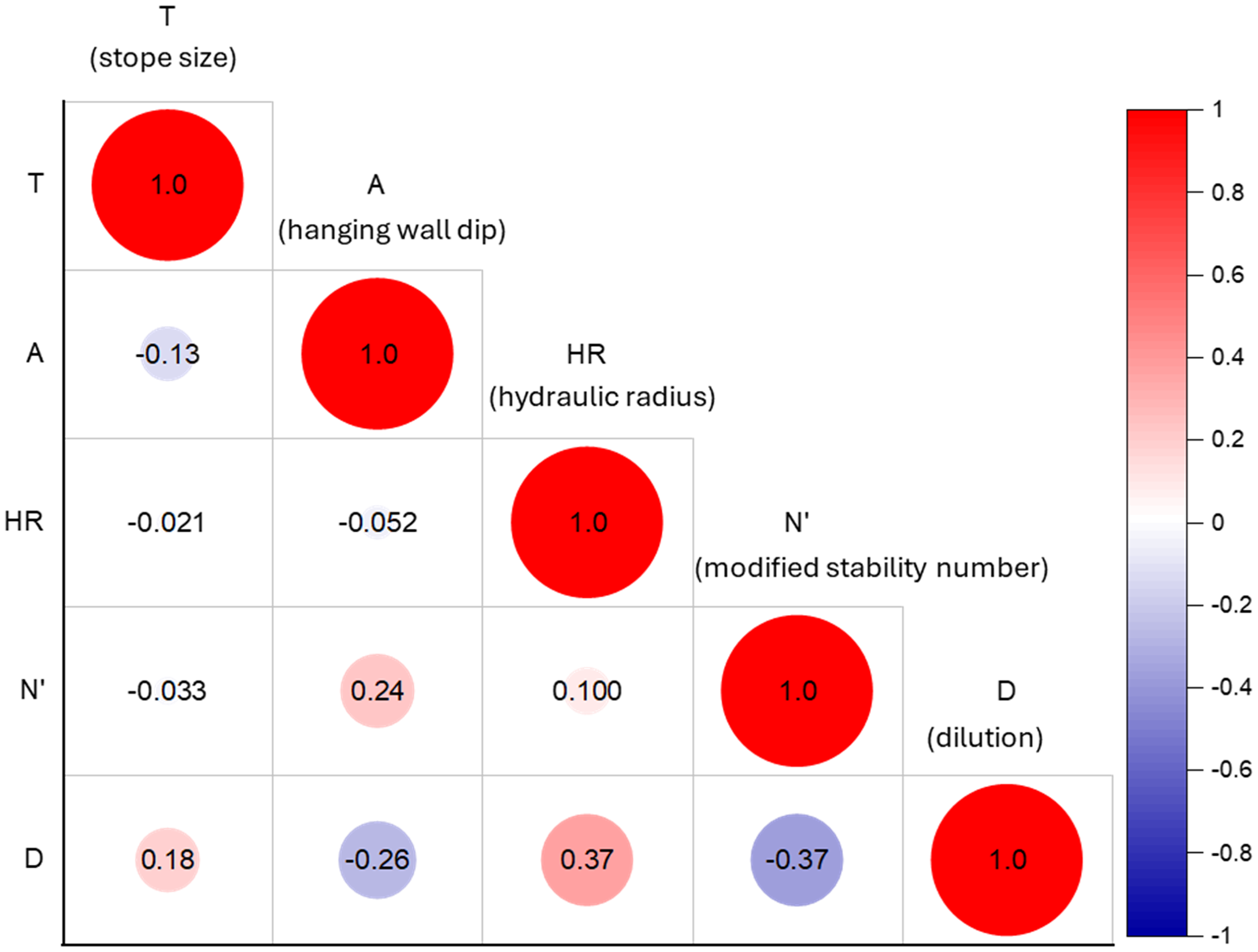
Correlation matrix for the dependent and independent variables.

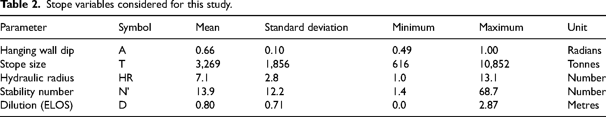
Histogram plots for the dependent variables showed that the distributions were largely asymmetrical as the stopes were from different reefs with dissimilar wide-ranging geometrical and geotechnical attributes. As such, a data contextualisation approach was adopted to ensure that the observed asymmetry was not error-driven, but represented inherent variability of data and a legitimate population of stopes that the model will still encounter and expected to predict dilution on. This approach involved additional checks and validations on the primary data sources, such as borehole logging and stope design data, to deal with outliers and noted anomalies. Further, these checks were critical to ensure the models would be trained on a realistic data profile that would enhance the models’ projective capability and generalisability. Measurements outside the data’s interquartile bounds, Q1 − 3(Q3 − Q1) and Q3 + 3(Q3 − Q1), where Q1 and Q3 represent the data's first and third quartiles, are generally regarded as extreme outliers that require to be removed to avoid skewing of data (Faradonbeh and Monjezi, 2017). A total of 29 cases were removed from the original data set following the completion of the data processing phase (i.e. missing values, outliers and unvalidated discrepancies), and 138 cases were kept for the study. A summary of the descriptive statistics for the final data set is presented in Table 2, and an overview of the distribution is presented graphically in the form of histograms in Figure 3.

Figure 3.

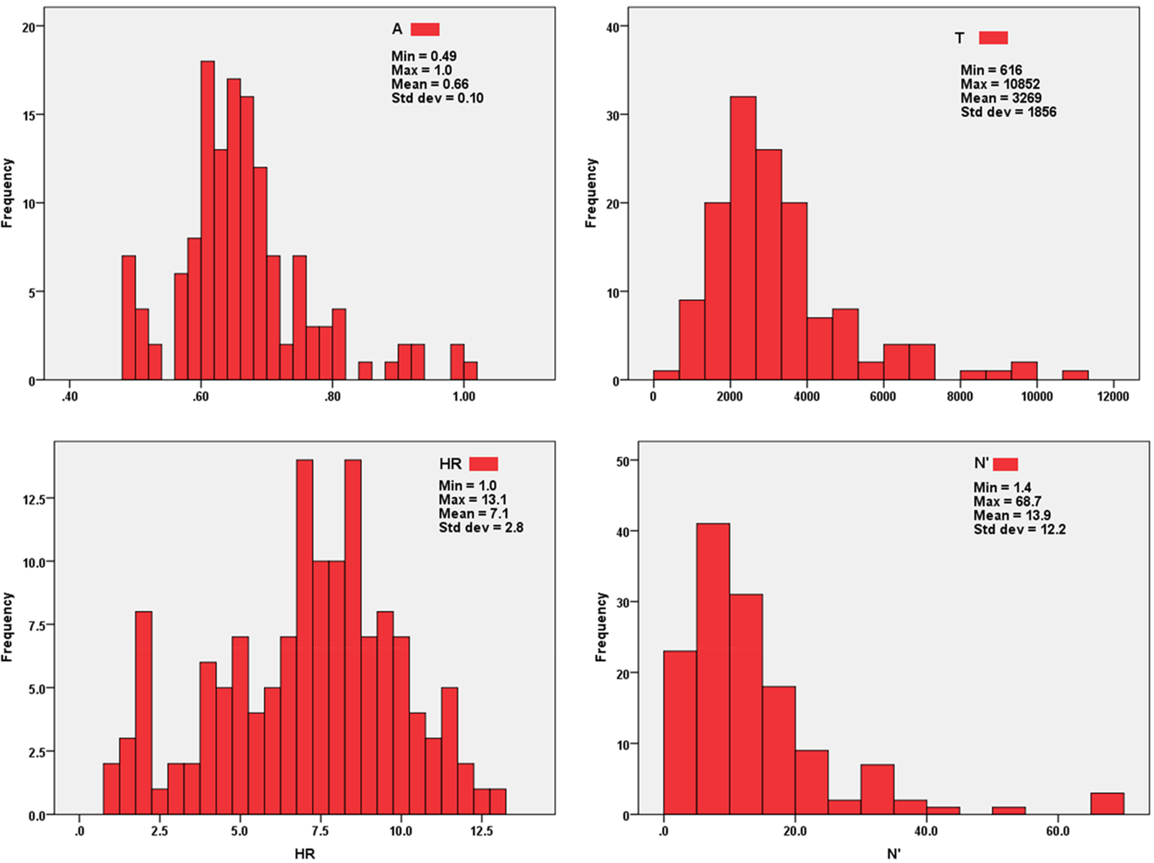
Histograms showing the statistical distribution of input data.

Table 2.

Stope variables considered for this study.

Parameter	Symbol	Mean	Standard deviation	Minimum	Maximum	Unit
Hanging wall dip	A	0.66	0.10	0.49	1.00	Radians
Stope size	T	3,269	1,856	616	10,852	Tonnes
Hydraulic radius	HR	7.1	2.8	1.0	13.1	Number
Stability number	N'	13.9	12.2	1.4	68.7	Number
Dilution (ELOS)	D	0.80	0.71	0.0	2.87	Metres

The sample data was then randomly shuffled several times before splitting it using the 80/20 rule for the training and validation or training and test sets. Accordingly, 115 samples from the shuffled data set were used as a training and validation set, and the remaining 23 samples were held out as a test set.

Methods and model development

Figure 4 presents a conceptual framework for the dilution prediction model construction followed in this study. It shows the generalised relationships between input variables, key processes and the independent variable. This framework sets the overarching philosophy to which all the proposed models will generally relate.

Figure 4.

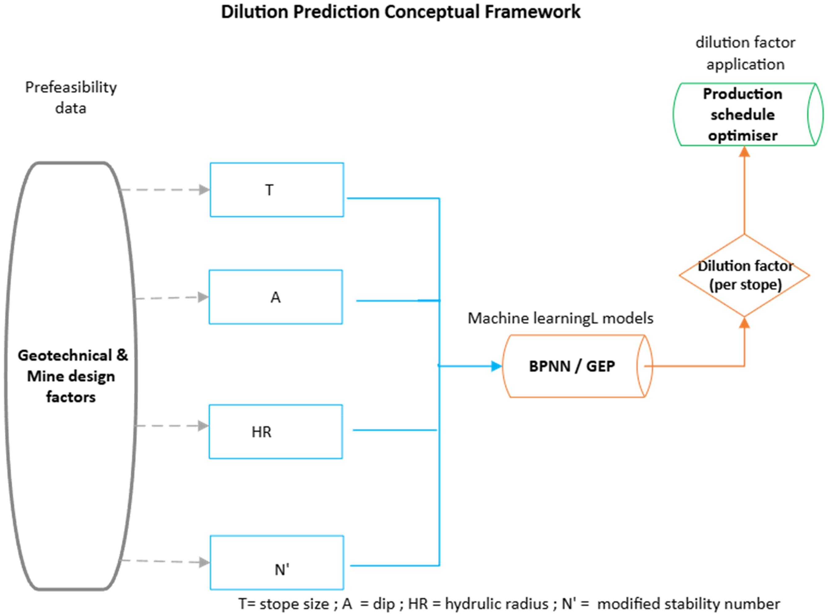
A generalised conceptual framework of the study.

Backpropagation artificial neural network (BPNN) algorithm

The three-layer structure backpropagation neural network has been shown to have strong approximation abilities for non-linear relationships in related mining studies (Lawal, 2020; Zhao and Jia’an, 2020). The model architecture comprises three layers: the input, hidden and output. A summary of the model's design and prediction is provided. However, the reader is directed to Li et al. (2021) and Zheng et al. (2022) for more comprehensive information on the algorithm's design. In the backpropagation algorithm, input data is processed through a transfer function through the hidden layer in a forward pass to the output layer. The output is compared to the measured target value, and the error variance is relayed back to the network in a backward pass to adjust synaptic weights, triggering an update to the model's input weights to reduce the output error to within set limits (Greenwood, 1991). Thus, ANN prediction optimisation fundamentally involves establishing optimum weights for inputs to achieve convergence below minimum set error limits. The input weights and bias of the optimised model are then used to establish a mathematical equation that represents the relationships between the inputs and the outputs.

BPNN model construction

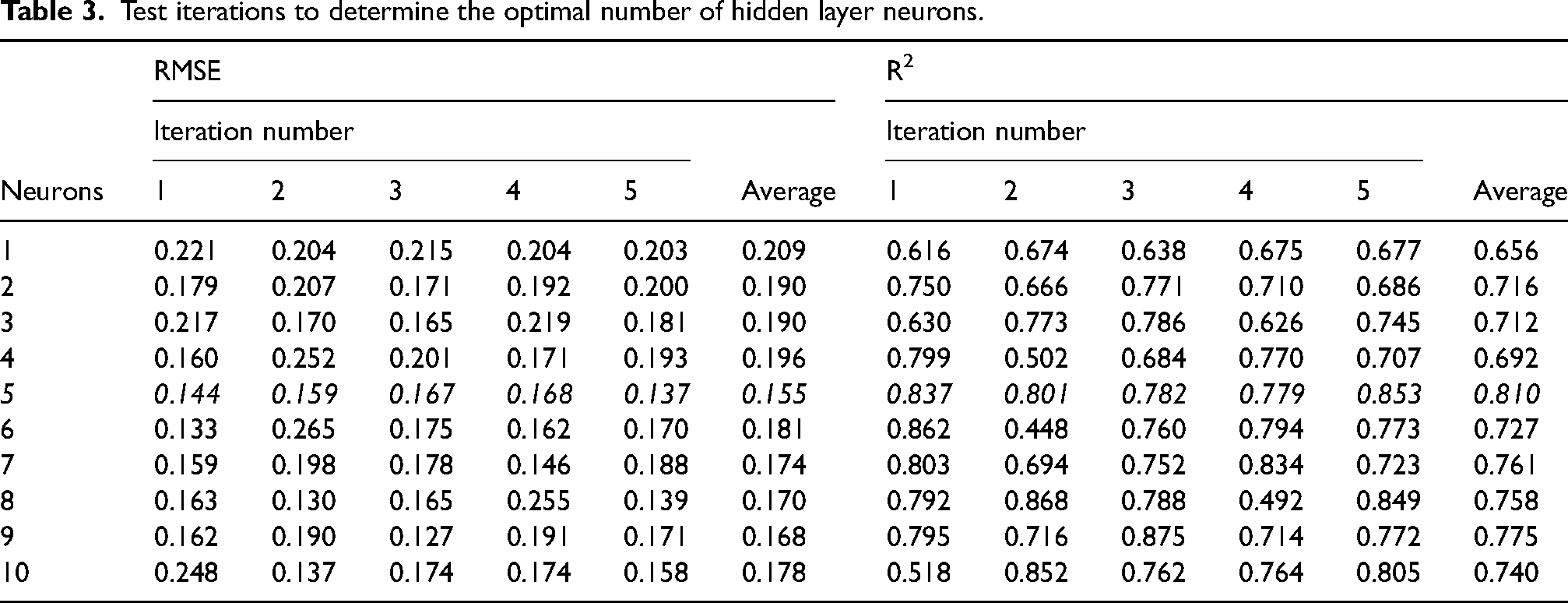
Extant literature on ANN model development has no universally prescribed method for determining the optimal number of neurons for the hidden layer. However, one widely used method is the trial and error approach, and this was adopted for this study. This involved iterative test runs to test various configurations as proposed by Gorman and Sejnowski (1988). MATLAB^® was used to determine the number of hidden neurons for a range of 1–10 neurons by performing test runs in an iterative loop and assessing performance, seeking to establish a neuron architecture with the least RMSE. The lowest RMSE value was achieved with five neurons in the hidden layer (Table 3).

Table 3.

Test iterations to determine the optimal number of hidden layer neurons.

	RMSE						R²
	Iteration number						Iteration number
Neurons	1	2	3	4	5	Average	1	2	3	4	5	Average
1	0.221	0.204	0.215	0.204	0.203	0.209	0.616	0.674	0.638	0.675	0.677	0.656
2	0.179	0.207	0.171	0.192	0.200	0.190	0.750	0.666	0.771	0.710	0.686	0.716
3	0.217	0.170	0.165	0.219	0.181	0.190	0.630	0.773	0.786	0.626	0.745	0.712
4	0.160	0.252	0.201	0.171	0.193	0.196	0.799	0.502	0.684	0.770	0.707	0.692
5	0.144	0.159	0.167	0.168	0.137	0.155	0.837	0.801	0.782	0.779	0.853	0.810
6	0.133	0.265	0.175	0.162	0.170	0.181	0.862	0.448	0.760	0.794	0.773	0.727
7	0.159	0.198	0.178	0.146	0.188	0.174	0.803	0.694	0.752	0.834	0.723	0.761
8	0.163	0.130	0.165	0.255	0.139	0.170	0.792	0.868	0.788	0.492	0.849	0.758
9	0.162	0.190	0.127	0.191	0.171	0.168	0.795	0.716	0.875	0.714	0.772	0.775
10	0.248	0.137	0.174	0.174	0.158	0.178	0.518	0.852	0.762	0.764	0.805	0.740

Accordingly, a five-neuron configuration for the hidden layer was adopted as the optimal neuron architecture for the BPNN model (Figure 5). The input layer has four neurons corresponding to the study's proposed input variables. The output layer has one neuron representing the output, i.e. ELOS equivalent dilution (D). K-fold cross-validation (CV) was used to split the data into subsets (k-folds) on which the model was then trained and validated ‘k’ times instead of a single run. Cross-validation was essential to avoid overfitting the model and ensure that the model's performance could be generalised on unseen data and, therefore, appropriate for prediction purposes. Specifically, a five-fold CV was applied to split the training set into five subtraining sets (five-folds). In each iteration, data from four folds (80% of the training set) was trained and then validated on unseen data from the remaining fold (20%). A low learning rate of 0.001, a target error threshold of 10⁻², a maximum number of training epochs without change of 100 and maximum training iterations of 10,000 were used to ensure effective model training. Further, the model's independent variables were also normalised to the [0,1] range to improve the dimensional consistency of inputs and ensure compatibility with the selected activation function.

Figure 5.

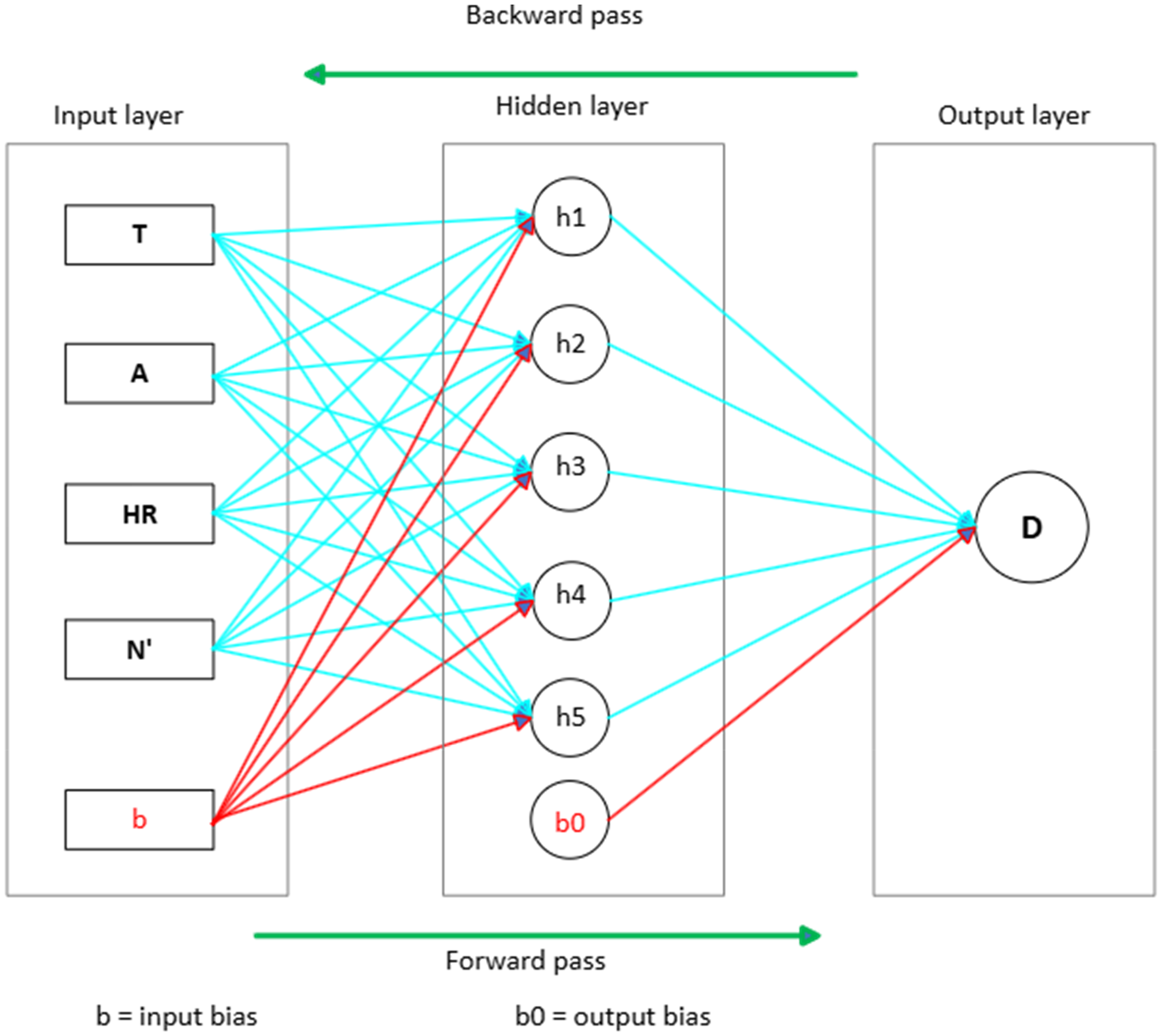
ANN model architecture showing the layers, neurons and dual propagation directions.

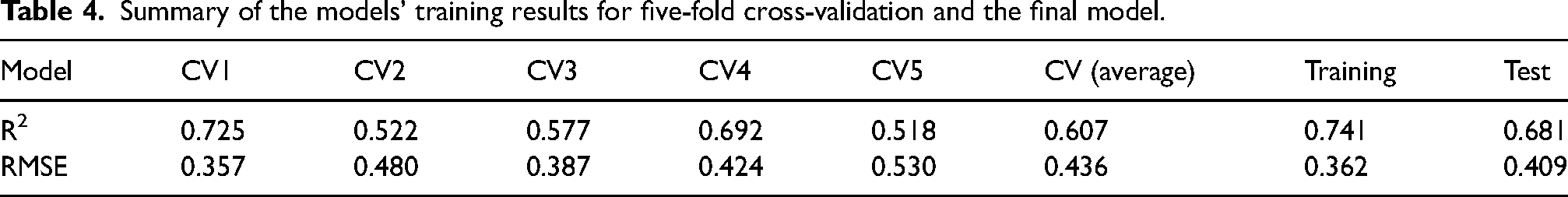
The network model was built using the Origin Lab^® software. The software has a simplified user interface with a wide range of optionalities on input data settings and output display, providing great flexibility in training neural network models. A key feature of the software is its default capability to normalise or standardise inputs in the background for network training but still keep the output (predictions) in their original, unscaled form. As such, the formulated proxy regression equation will also be in the same format to effectively simulate the training environment for optimum performance. Model tuning was conducted by trialling different activation functions (logistic, identity, hyperbolic tangent and rectified linear unit) and assessing the model's performance. The best training and validation performance was achieved using the logistic activation function (the sigmoid function), with an average $R^{2}$ of 0.61 and an $R M S E$ of 0.436 for all folds. The results of the final model, trained on the entire training set, suggest the model harnessed the acquired learning during the CV, resulting in an improved $R^{2}$ of 0.74, and the $R M S E$ improved to 0.409. Table 4 summarises the training results for the five-fold CV and the final model.

Table 4.

Summary of the models’ training results for five-fold cross-validation and the final model.

Model	CV1	CV2	CV3	CV4	CV5	CV (average)	Training	Test
R²	0.725	0.522	0.577	0.692	0.518	0.607	0.741	0.681
RMSE	0.357	0.480	0.387	0.424	0.530	0.436	0.362	0.409

The sigmoid activation function, which is defined mathematically as

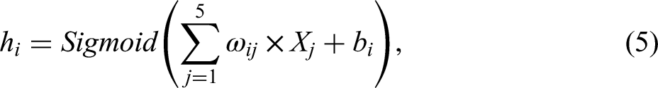
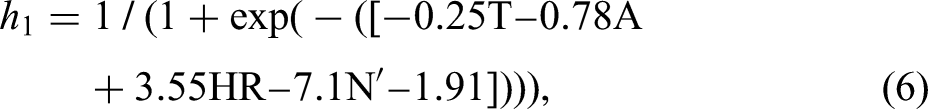
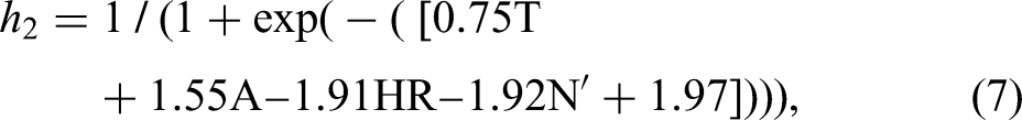
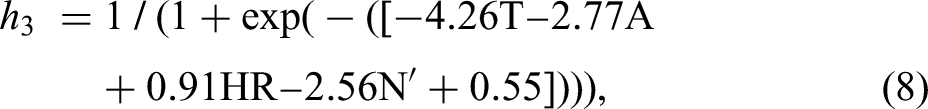
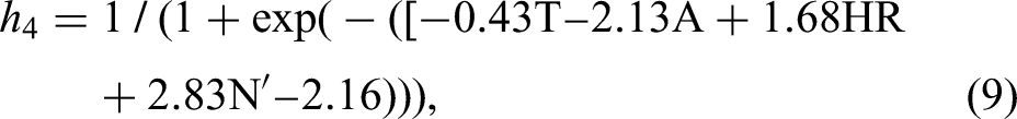
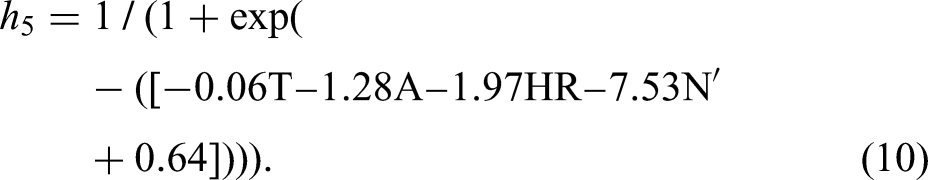
Logistic (x) = $\frac{1}{[1 + \exp (- x)]}$ , maps the normalised inputs ( $X_{1}$ , $X_{2}$ , …, $X_{4}$ ) to the hidden layer and calculates the value of each hidden neuron according to equation (5):

h_{i} = S i g m o i d (\sum_{j = 1}^{5} ω_{i j} \times X_{j} + b_{i}),

(5)where

h_{i}

is the calculated value of the hidden layer neurons,

w_{i j}

represents input

j

’s weight to the hidden layer neuron i, and

b_{i}

is the bias factor for the hidden neuron i. The weights of the optimised model were extracted and used to calculate the model's hidden neuron coefficients (i.e.

h_{1}

h_{5}

), as presented by equations (6) to (10): :

h_{1} = 1 / (1 + \exp (- ([- 0.25 T – 0.78 A + 3.55 HR – 7.1 N^{'} – 1.91]))),

(6)

h_{2} = 1 / (1 + \exp (- ([0.75 T + 1.55 A – 1.91 HR – 1.92 N^{'} + 1.97]))),

(7)

h_{3} = 1 / (1 + \exp (- ([- 4.26 T – 2.77 A + 0.91 HR – 2.56 N^{'} + 0.55]))),

(8)

h_{4} = 1 / (1 + \exp (- ([- 0.43 T – 2.13 A + 1.68 HR + 2.83 N^{'} – 2.16))),

(9)

h_{5} = 1 / (1 + \exp (- ([- 0.06 T – 1.28 A – 1.97 HR – 7.53 N^{'} + 0.64]))) .

(10)

The output from the hidden layer (i.e. predictions) is calculated using the formula below: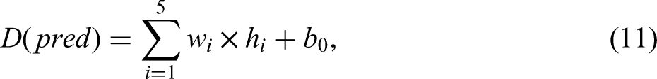

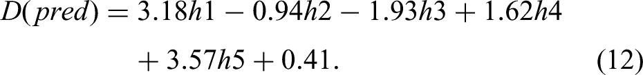
D (p r e d) = \sum_{i = 1}^{5} w_{i} \times h_{i} + b_{0},

(11)where

D (p r e d)

is the predicted output,

w_{i}

are the weights from the hidden layer neurons to the output neuron and

b_{0}

is the bias for the output layer. Substituting equations (6) to (10) into equation (11), the model's prediction equation is mathematically represented as follows:

D (p r e d) = 3.18 h 1 - 0.94 h 2 - 1.93 h 3 + 1.62 h 4 + 3.57 h 5 + 0.41.

(12)

If required to calculate dilution with the original unnormalised inputs, then equation (12) will need to be back-transformed by replacing the normalised values in equations (6) to (10) with the actual values using equation (13):

x^{'} = \frac{X - X_{m a x}}{X_{m a x} - X_{m i n}},

(13)where for a given input data set of a variable X,

x^{'}

is the normalised value and

X_{m a x}

and

X_{m i n}

are the minimum and maximum values for the variable X. Thus, the model's back-transformed prediction equation is then presented in equation (14) as follows:

D (p r e d) = 3.18 H 1 - 0.94 H 2 - 1.93 H 3 + 1.62 H 4 + 3.57 H 5 + 0.41,

(14)where

H 1, H 2, . ., H 5

represent the model's hidden neuron coefficients calculated using the original unnormalised values by replacing the normalised values using equation (13).

Gene expression programming algorithm

Gene expression programming (GEP) is a genome–phenome nature-inspired genetic algorithm that integrates the simplicity of the legacy genetic algorithms and the proficiencies of genetic programming (Roohollah Shirani et al., 2017) to decipher relationships between variables and use the acquired knowledge to explain the relationships (Ferreira et al., 2002). The model allows user-defined fitness functions to evaluate the initial randomly generated population of linear-coded fixed-length strings of different sizes (chromosomes) that use the Karva code language to interpret and express coded programs. The chromosomes comprise genes with a head and a tail and can also be presented as expression trees (ETs). Terminals (input variables and constants) and functions (mathematical functions) in the head instantiate chromosome modification through processes such as mutation, inversion or transposition (Mohammadpour, 2017). These modifications to the selected population generate a new population with new characteristics. Preference for reproduction is accorded to the fittest chromosomes. This process repeats on the new population until a suitable solution is achieved or stopping criteria are met. A concise description of the key stages of GEP is presented; however, for a detailed scope, the reader is directed to the comprehensive treatise by Ferreira et al. (2002). The GEP algorithm has six key steps, as outlined below and graphically presented in Figure 6.

Establishment of the functions and terminals that govern the formation of chromosomes

Selection of a fitness function for model performance evaluation (the $R M S E$ fitness function was used)

Random generation of the initial population using functions and terminals

Evaluation of the chromosomes’ fitness using the selected fitness function (RMSE)

Selection and retention of best chromosomes for replication in the next generation

The modification of chromosomes through genetic operators and their rates (mutation, inversion, transposition, recombination) and combining reproduced chromosomes with retained best chromosomes to create the next generation of chromosomes

Figure 6.

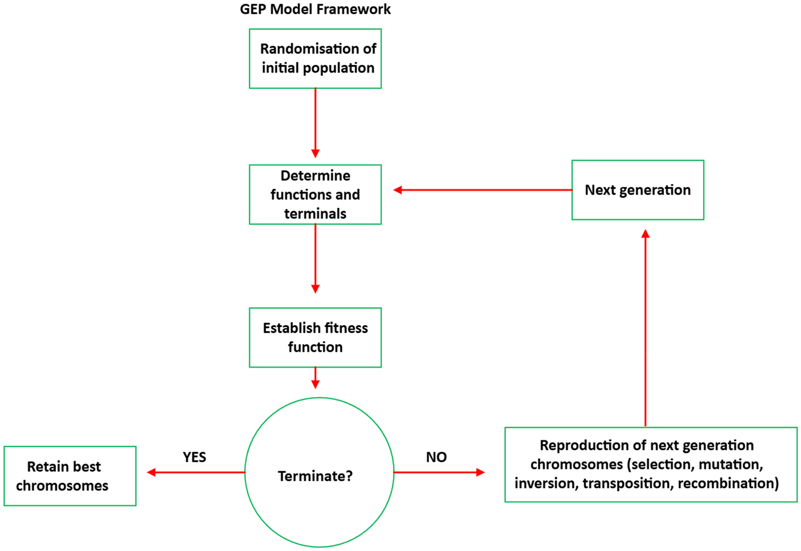
Generalised schematic of the GEP model framework.

The process repeats through a closed-loop iteration between steps iv, v and vi until the circuit is broken by achieving the set fitness condition, or a number of generations. At this point, the optimal solution is reached.

GeneXproTools software version 5.0 was used to build the model. The software is a powerful tool with exceptionally high flexibility in modelling functions and optionality that can quickly generate prediction models once the data is processed and provided in the required format. Several iterations were conducted using different genetic linking functions (i.e. ×, /, +, −) as part of model tuning, and finally, the addition (+) linking function was selected based on comparative performance results. The maximum generation was set at 3000 to avoid overtraining, which could result in overfitting the model. Further, model performance trial runs conducted using either the actual or normalised inputs yielded similar results, leading to conclude that input data transformation was not necessary. Random shuffling was used based on the 80/20 rule for subsplitting the original training set (115 samples) into a training (92 samples) and validation set (23 samples). After establishing the model's optimal settings, the parameters and settings eventually adopted are presented in Table 5.

Table 5.

Parameters, tuning range and the final settings used for the GEP model.

Parameter	Range	Setting
Fitness function		RMSE
Number of generations	1000–3000	3000
Number of chromosomes		256
Head size		8
Number of genes		3
Linking function		Addition
Mutation rate		0.00138
Inversion rate		0.00546
Gene transposition rate		0.00277
Gene recombination rate		0.00277
Data partition (training/validation)		Random
Data partition ratio (training/validation)	%	80/20

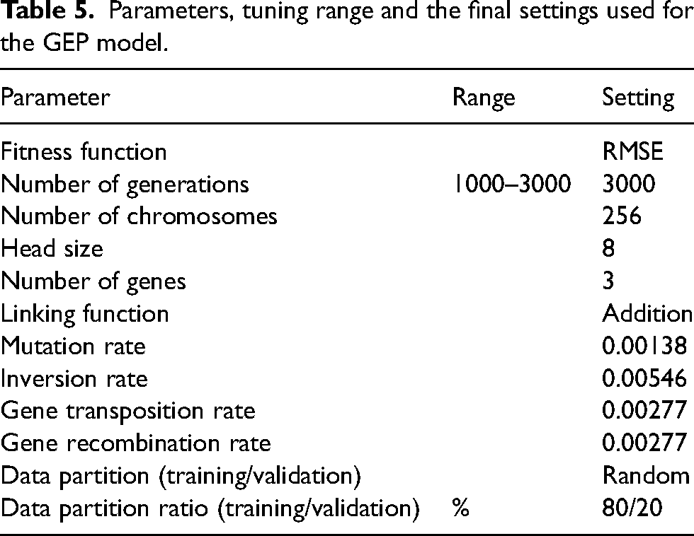
Five consecutive runs were conducted on these settings, with a random split of the entire training data set of 115 samples using the 80/20 rule to split it into a subset of a new training and validation set with 92 (80%) and 23 (20%) samples, respectively. The results of the consecutive training iterations are summarised in Table 6.

Table 6.

Summary of the GEP models’ training and validation results.

		Iteration number
Model		1	2	3	4	5	Average
Training	R²	0.765	0.738	0.750	0.783	0.741	0.755
Training	RMSE	0.355	0.372	0.364	0.340	0.370	0.360
Validation	R²	0.690	0.727	0.661	0.785	0.777	0.728
Validation	RMSE	0.351	0.326	0.375	0.354	0.342	0.350
Average	R²	0.727	0.733	0.705	0.784	0.759	0.742
Average	RMSE	0.353	0.349	0.370	0.347	0.356	0.355

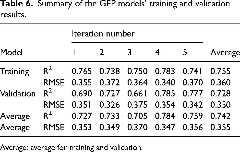
Average: average for training and validation.

It is clear that model 4 has the best performance based on the highest R² across both the training and validation set and its MSE values that are broadly in line with the model's average. Also, the average performance for training and validation shows that model 4 has the highest average R² and the least RMSE. Accordingly, model 4 was selected for further analysis.

The best GEP-based solution (model 4) resulted in a chromosome with three sub-ETs (genes), as shown in Figure 7. The values T, A, HR and N′ represent the model's inputs, and the numbers in the leaf nodes are constants generated by the model to enhance effective modelling of relationships between genes.

Figure 7.

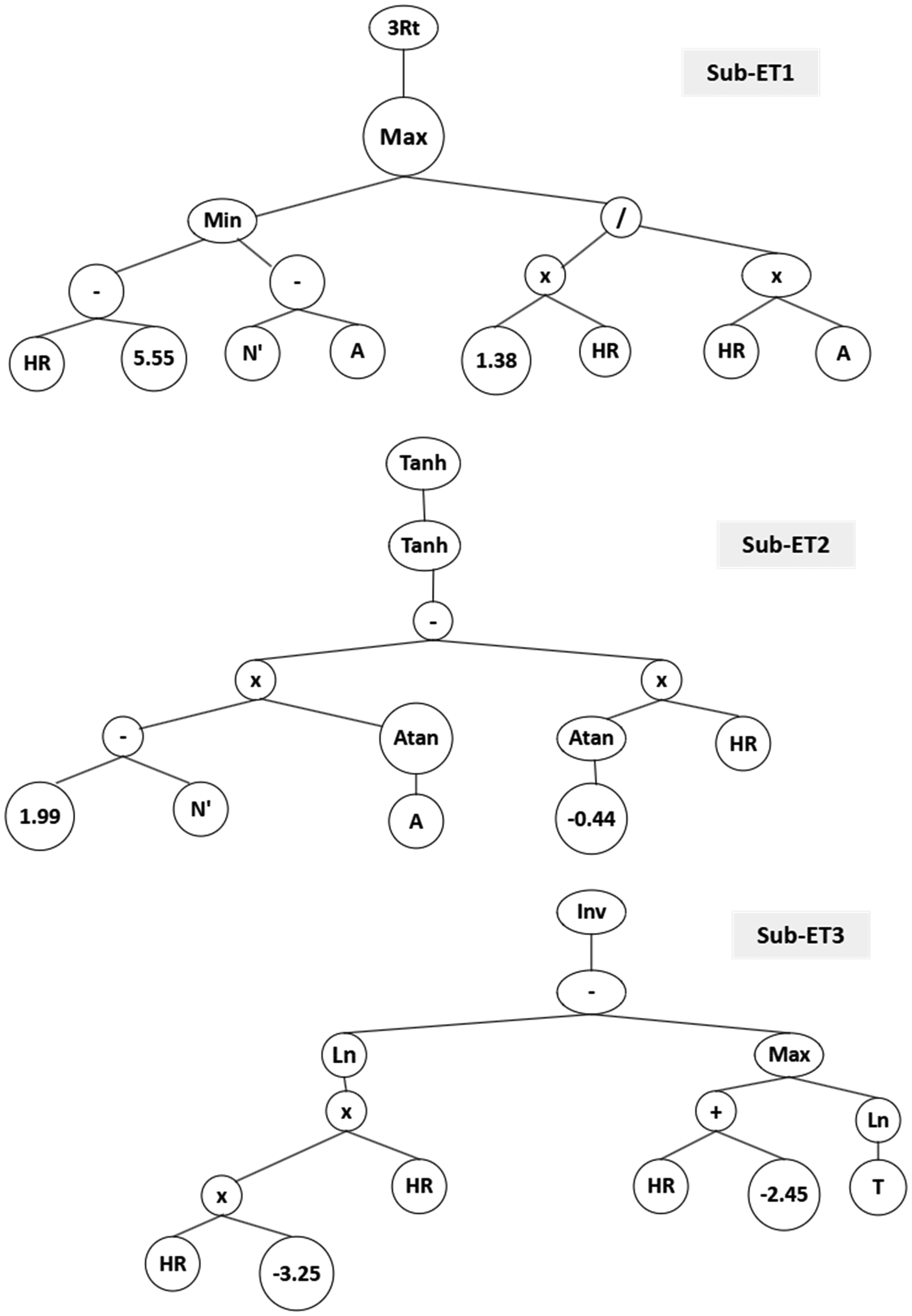
Expression tree (ET) for the GEP model.

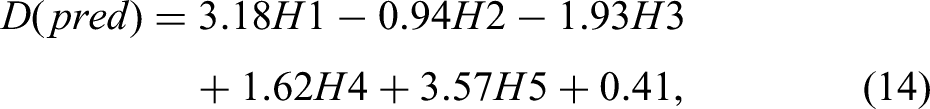
The mathematical equations for the three genes (sub-ETs) were then extracted and summed up (as per the addition linking function) to get the output using equation (15):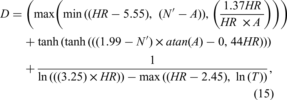

D = (max (min ((H R - 5.55), (N^{'} - A)), (\frac{1.37 H R}{H R \times A}))); (\frac{1}{3}) + \tanh (\tanh (((1.99 - N^{'}) \times a t a n (A) - 0, 44 H R))) + \frac{1}{\ln (((3.25) \times H R)) - max ((H R - 2.45), \ln (T))},

(15)

subject to $c^{\frac{1}{3}} = {\begin{matrix} - {(- c)}^{\frac{1}{3}} i f c < 0 \\ c^{\frac{1}{3}} i f c > 0 \end{matrix}$ , where c is the first part of equation (15) to which the cube root function is executed.

The expression tree (ET) displays how the inputs are combined with different mathematical functions to visually depict the construction of the non-linear equation that predicts the output for a given set of inputs. This simplifies an otherwise black-box operation, allowing the prediction process to be visually conceived from the expression tree, as in decision tree models’ architecture. In an actual mining scenario, this can facilitate easier analysis of complex interdependencies amongst the models’ input variables, thereby enhancing rapid assessment of the sensitivity of the predicted value to the inputs.

The extracted equation was then tested on the test set, and the results were compared with the actual model. The results are discussed in the next section.

Results and discussion

The root mean square Error $(R M S E)$ , coefficient of determination ( $R^{2}$ ) and the correlation coefficient $(R)$ are introduced to assess the performance of models. The performance results of all models were summarised and presented in Table 7, showing the comparative performance based on the selected metrics (R² and RMSE).

Table 7.

Summary of performance results for all models.

	BPNN			GEP
Fitness	Training model	Test model	BPNN equation test model	Training model	Test model	GEP equation test model
R	0.861	0.825	0.825	0.885	0.86	0.86
R²	0.741	0.681	0.681	0.783	0.74	0.74
RMSE	0.362	0.409	0.409	0.34	0.369	0.369

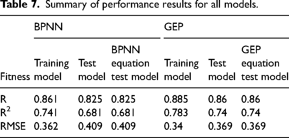
The summary results show a correlation coefficient between 82% and 88% for ELOS for both BPNN and GEP dilution prediction. These findings generally align with previous related studies (Chongchong et al., 2018; Jang et al., 2015), even though this study considered fewer variables than previous studies. Thus, the improved results provide alternative means for establishing robust, generalisable dilution estimates for production planning and scheduling devoid of bias from drill and blast inputs or other related metrics.

The mathematical proxy models’ prediction results perfectly match those obtained by the models on the test data (Table 7), confirming the successful mathematical simulation of both the BPNN and GEP models. The models’ mathematical proxies bring to view a crystallised perspective of the computations and complex relationship, which are often buried in the actual models’ complex architectures, commonly referred to as ‘black box’ due to their complexity. Indeed, this perspective is shared by Hotelling (1991), who argues that mathematics systematically unpacks the relationships, and nothing has a richer profusion of application or traverses the whole domain of human knowledge as does mathematics. Model configuration to mathematical proxies provides improved clarity and visualisation of the interlinked relationships, allowing engineers and operators to understand the key drivers of dilution better and, therefore, focus early on secondary controls for minimising the deviation of production schedules downstream at the mining stage.

The BPNN and GEP proxy models’ predicted dilution values on the test data set were plotted against the measured values for each stope to explore further insights on the model's predictions. Figure 8 overviews the model's predictions on a per-stope fidelity.

Figure 8.

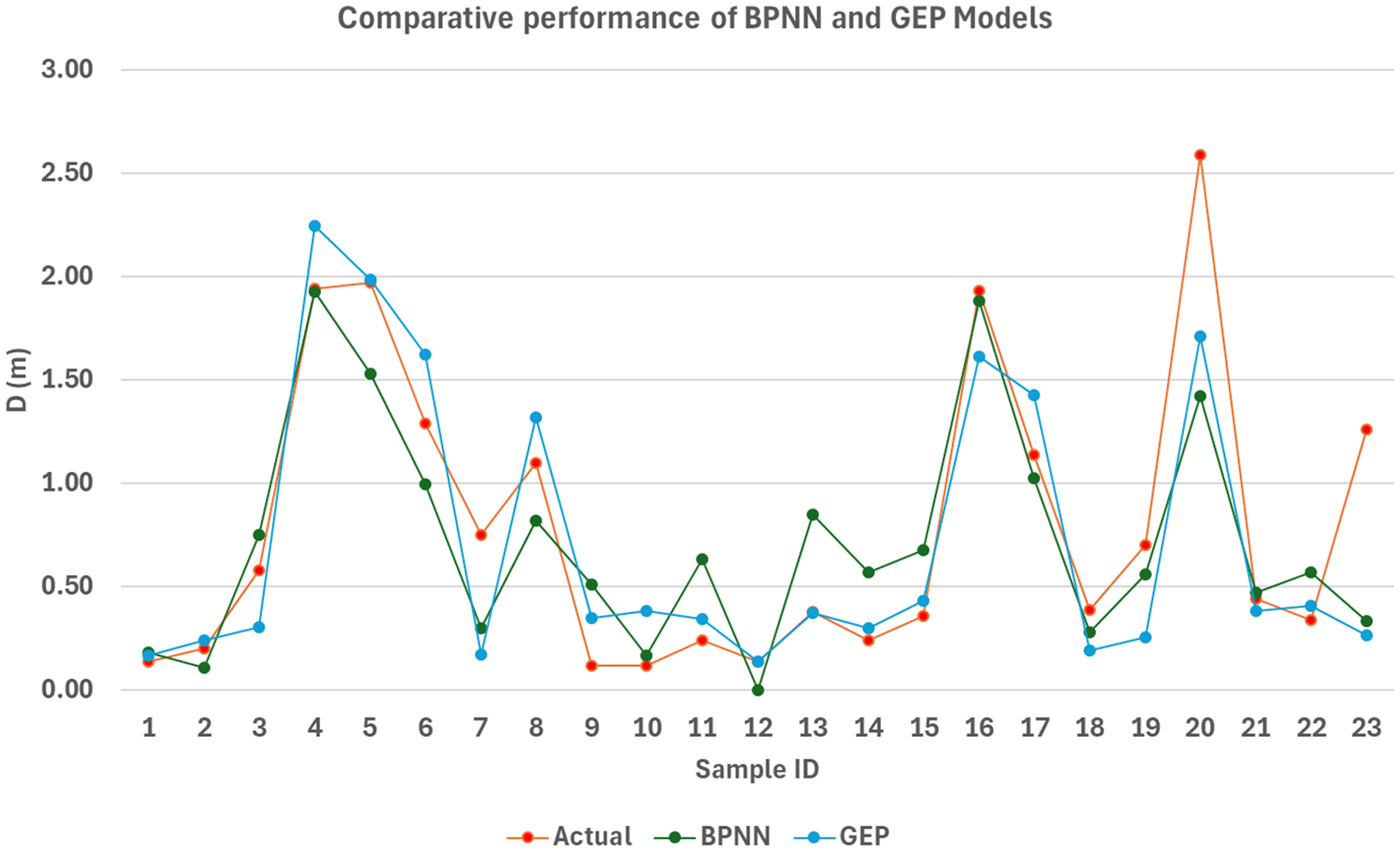
BPNN and GEP models’ predictions against the measured values on the test data set.

The analysis of the model's prediction on a per-stope basis showed that both models’ sensitivity was generally low in the regions towards the extreme values, i.e. when ELOS values approach the minimum or maximum values of the ELOS dilution spectrum used for the study (i.e. 0.0 and 2.87). However, this is considered inconsequential in practical application because ELOS dilution in the lower spectrum is generally classified as minimal dilution that may not be avoidable due to blast damage. Similarly, ELOS dilution values approaching the higher end of the spectrum are considered extreme cases, with an ELOS above 2 also generally regarded as a failure criterion rather than mining dilution. Further, this observation is consistent with extant literature findings on dilution, confirming that the relationship between dilution and stability parameters such as the stability number and hanging wall radius is best modelled by a logistic function. To clarify this behaviour, Figure 9 offers an overview of the general form of the logistic function, showing the insensitive regions towards the low- and high-end values of the spectrum range.

Figure 9.

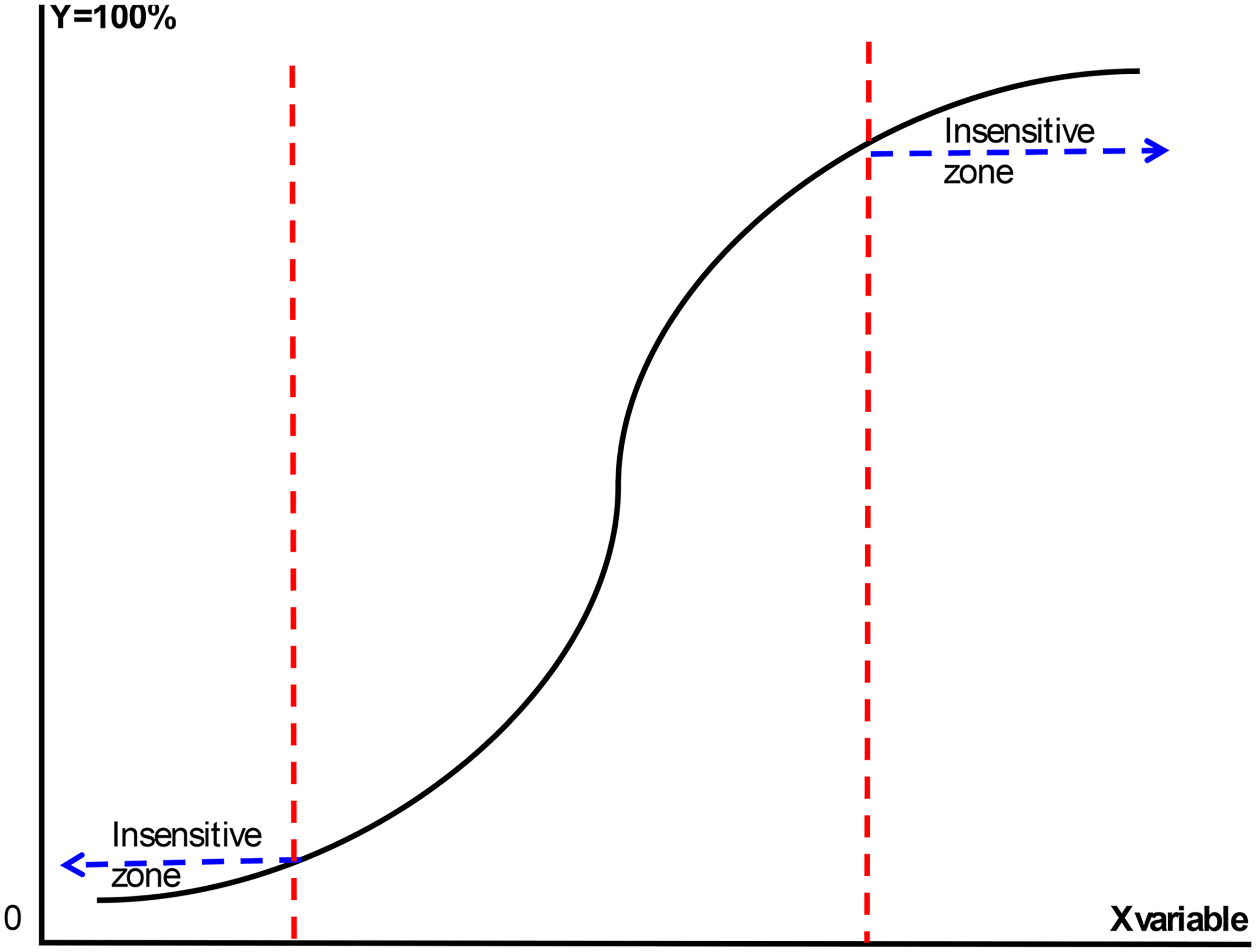
Generalised logistic regression graph showing low sensitivity at lower and upper bounds.

While stability is generally defined in terms of short-term stability, in a sense, it is mostly influenced by the mining methods that, by their nature, are of short-term duration. Thus, the failure criterion, which represents stope hanging wall failure and unstable ground conditions where it is deemed unsafe to conduct mining activities (Brady et al., 2005), does not pass the litmus for stable mining conditions, a fundamental assumption that must be met for mining operations. Thus, while the models are less sensitive in these regions, the predictands achieved are deemed sufficient to provide an indicative estimate for mine planning and production scheduling purposes.

These results also point to the difficulty in predicting the actual ground conditions in the mining zone, which may compromise the prediction accuracy of the models. As such, the models must be updated often to mitigate this as new data is generated. Overall, while there might appear to be a blurred distinction between the models’ performance on the test set as the results were considerably at par, the GEP model has exceptionally high flexibility on model inputs and similar prediction results obtained using actual and normalised input data are a testimony to that fact. Based on the foregoing, the GEP model was recommended for deployment based on its superior prediction accuracy, better generalisation capability and minimal data transformation requirements.

Infield application and further validation of the GEP proxy model

To further assess the performance of the GEP proxy model (i.e. the GEP model's mathematical equation), the model was tested on a sample of three recently completed stopes in the same mining area where the training and test data were extracted. The test stopes’ parameters and the proxy model's prediction results are summarised in Table 8.

Table 8.

GEP proxy model's prediction results on test stopes.

Test stope	T	A	HR	N′	D (measured)	D (predicted)	Relative error deviation (%)
1	1924	0.66	8.4	27.2	0.23	0.19	19.1
2	3053	0.49	6.9	19.6	0.35	0.31	11.7
3	2505	0.79	4.7	14.0	0.13	0.16	24.8

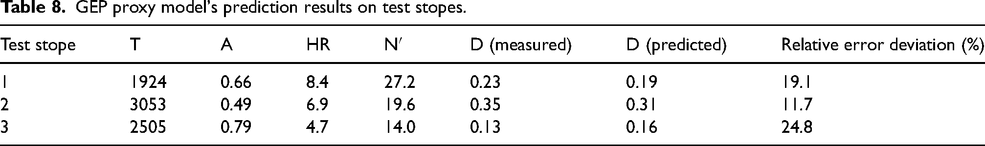
The preliminary test results show that the model's predictions were within a 10–30% relative error margin, consistent with the model's prediction accuracy range established in the model testing and validation phases.

GEP model field deployment and preliminary results

Having selected the GEP model as the best model, the model was deployed for further tests on an additional sample of 64 stopes acquired from another section of the mine where mining occurs on a different orebody of similar dimensions using the open stoping mining method. The summary statics details of the sample data are provided in Table 9.

Table 9.

Summary statistics for the GEP field sample.

Parameter	Symbol	Mean	Standard deviation	Minimum	Maximum	Unit
Hanging wall dip	A	0.63	0.08	0.44	0.79	Radians
Stope size	T	2,898	1,107	1,251	7,142	Tonnes
Hydraulic radius	HR	7.67	1.74	3.2	10.2	Number
Stability number	N′	10.7	6.8	4.9	39.1	Number
Dilution (ELOS)	D	0.76	0.41	0.12	1.90	Metres

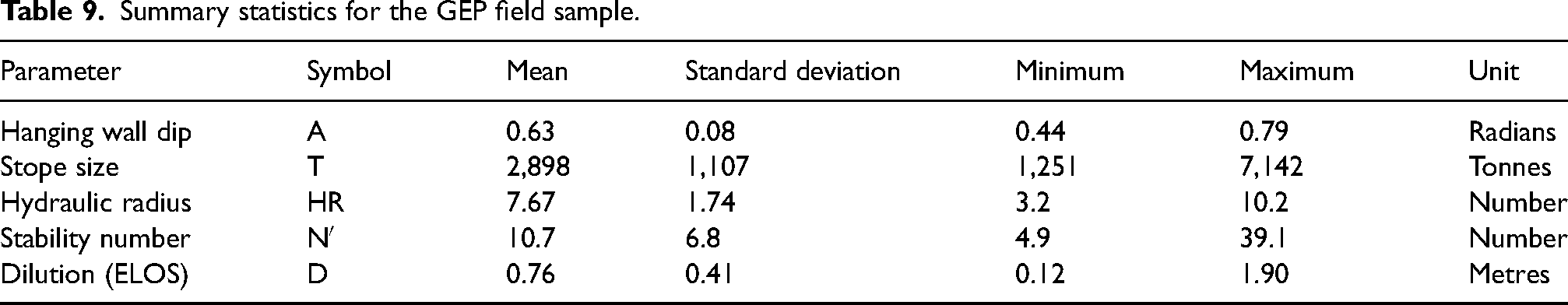
The model's performance on the additional sample showed an R and $R^{2}$ values of 0.83 and 0.70, respectively, with an RMSE of 0.24. These results closely mirrored the model's test results established during the training and testing phases, with a slight variance of under 10%, which suggests that the model is fairly robust for dilution prediction to support mine planning activities at the strategic level of detail.

Merits and limitations of the models

The simplicity of the GEP model's output interpretation in a tree structure form, coupled with its high performance, speed, accuracy and minimal data transformation requirements, renders itself a preferred model of choice over other models with complex black-box architecture. Notwithstanding their comparative performance and the black-box nature of the actual models, the ability to extract proxy equations brings unparalleled convenience for users to deploy the models to Excel spreadsheets for use as an everyday tool. Further, these proxy models may also be linked as an input model to other optimisation models, such as production scheduling, enabling a seamless integration of optimisation processes.

However, although the models’ performance may be regarded as sufficient for mine planning at the strategic level of detail and accuracy, the model's performance will still be limited to the range of input parameters used to develop the models. Additionally, it may be worthwhile for future studies to include drill and blast factors and assess if the model's prediction accuracy can be further enhanced without compromising the model's generalisability. Furthermore, the stopes’ geology and geotechnical databases at the case study site were mature, with sufficient data points for most of the stopes; hence, it may be difficult to achieve high prediction accuracy in new areas with low data density.

Conclusions

Two predictive ML models, namely, artificial neural network with backpropagation (BPNN) and gene expression programming (GEP), were developed to predict mining dilution on a per-stope basis based on geotechnical and geometrical stope design data. The test results showed that the GEP performed better, recording a coefficient of determination, R², of 0.740 with a root mean square error (RMSE) of 0.361 compared to BPNN's 0.681 and 0.409, respectively. The models were mathematically simulated to establish mathematical equations that were then used as proxy models. The proxy models were first tested on the test data, and the results obtained were similar to those achieved by the original respective models, confirming that the mathematically simulated proxies were as robust and effective for dilution prediction as the original software-run models. Further, preliminary results for field deployment of the GEP model showed that model performance was broadly consistent with the test results. Accordingly, the GEP model is recommended for dilution prediction for medium- to long-term production scheduling at the prescribed level of accuracy. The comparatively better performance of GEP models points to its growing maturity for mining-related applications, suggesting that it is well suited to handle prediction for similar and related studies. Importantly, the novel application of GEP for dilution prediction in open stoping operations enriches the existing literature on dilution prediction studies, marks another shift in revolutionising the conceptualisation of dilution prediction and sets the stage for future related studies. Future studies are also recommended to explore ways to improve prediction accuracy by harnessing the merits of improved data capturing, analysis and processing using emerging ML technologies in mining processes to enhance the granularity of model inputs.

Footnotes

Declaration of conflicting interests

The authors declared no potential conflicts of interest with respect to the research, authorship, and/or publication of this article.

Funding

The authors received no financial support for the research, authorship, and/or publication of this article.

ORCID iD

Prosper Chimunhu

References

Abdellah Wael

Hefni

Ahmed

(2020) Factors influencing stope hanging wall stability and ore dilution in narrow-vein deposits: Part 1. Geotechnical and Geological Engineering 38(2): 1451–1470.

Amirkiyaei

Ghasemi

Kadkhodaei

(2023) Development of empirical models to predict stope wall stability in open stope mines using gene-expression programming. Arabian Journal of Geosciences 16(11): 616.

Brady

Martin

Pakalnis

(2005) Empirical approaches for opening design in weak rock masses. Mining Technology (Transactions of the Institution of Mining and Metallurgy, Section A) 114(1): 13–20.

Buaba

, 2023. Application of machine learning techniques to estimate mine safety and health hazards for integration into underground production scheduling optimization . Ph.D.. South Dakota, United States: South Dakota School of Mines and Technology.

Cadenillas

, 2023. Prediction of unplanned dilution in underground mines through machine learning techniques . M.Sc.. Quebec, CA: Canada: McGill University (Canada).

Chimunhu

Faradonbeh

Topal

, et al. (2024a) Development of novel hybrid intelligent predictive models for dilution prediction in underground sub-level mining. Mining, Metallurgy & Exploration 41(4): 2079–2098.

Chimunhu

Topal

Ajak

, et al. (2022) A review of machine learning applications for underground mine planning and scheduling. Resources Policy 77: 102693.

Chimunhu

Topal

Ajak

, et al. (2024b) Chapter 11 – Underground mine planning and scheduling optimization: Opportunities for embracing machine learning augmented capabilities. In: Nguyen

Bui

X-N

Topal

, et al. (eds) Applications of Artificial Intelligence in Mining, Geotechnical and Geoengineering. Cambridge, MA: Elsevier, 183–195.

Chimunhu

Topal

Asad

MWA

, et al. (2024c) The future of underground mine planning in the era of machine learning: Opportunities for engineering robustness and flexibility. Mining Technology 133(4): 25726668241281875. doi: https://doi.org/10.1177/25726668241281875.

10.

Chongchong

Fourie

, et al. (2018) Prediction of open stope hangingwall stability using random forests. Natural Hazards 92(2): 1179–1197.

11.

Clark

(1998) Minimizing dilution in open stope mining with a focus on stope design and narrow vein longhole blasting. Vancouver, Canada: University of British Columbia.

12.

Delentas

Benardos

Nomikos

(2021) Analyzing stability conditions and ore dilution in open stope mining. Minerals 11(12): 1404.

13.

Faradonbeh

Monjezi

(2017) Prediction and minimization of blast-induced ground vibration using two robust meta-heuristic algorithms. Engineering with Computers 33(4): 835–851.

14.

Ferreira

Furuhashi

Köppen

, et al. (2002) Gene Expression Programming in Problem Solving. London, UK: Springer London, Limited, pp. 635–653.

15.

Forster

Milne

Pop

(2007) Mining and rock mass factors influencing hangingwall dilution. In: 1st Canada – U.S. Rock Mechanics Symposium.

16.

Gorman

Sejnowski

(1988) Analysis of hidden units in a layered network trained to classify sonar targets. Neural Networks 1(1): 75–89.

17.

Greenwood

(1991) An overview of neural networks. Behavioral Science 36(1): 1–33.

18.

Hefni

Abdellah Wael

Ahmed

(2020) Factors influencing stope hanging wall stability and ore dilution in narrow-vein deposits: Part II. Geotechnical and Geological Engineering 38(4): 3795–3813.

19.

Henning

, 2007. Evaluation of long-hole mine design influences on unplanned ore dilution . Ph.D.. Ann Arbor: McGill University (Canada).

20.

Henning

Mitri

(2008) Assessment and control of ore dilution in long hole mining: Case studies. Geotechnical and Geological Engineering 26(4): 349–366.

21.

Hotelling

(1991) The economics of exhaustible resources (reprinted from journal of political-economy, Vol 39, PG 137-175, 1931). Bulletin of Mathematical Biology 53(1-2): 281–312.

22.

Hughes

, 2011. Factors influencing overbreak in narrow vein longitudinal retreat mining . M.Eng.. Ann Arbor: McGill University (Canada).

23.

Jalilian

Ghasemi

Kadkhodaei

(2024) Stability assessment of open spans in underground entry-type excavations by focusing on data mining methods. Mining, Metallurgy & Exploration 41(2): 843–858.

24.

Jang

Topal

(2013) Optimizing overbreak prediction based on geological parameters comparing multiple regression analysis and artificial neural network. Tunnelling and Underground Space Technology 38: 161–169.

25.

Jang

Topal

Kawamura

(2015) Unplanned dilution and ore loss prediction in longhole stoping mines via multiple regression and artificial neural network analyses. Journal of the Southern African Institute of Mining and Metallurgy 115: 449–456.

26.

Jang

Topal

Kawamura

(2016) Illumination of parameter contributions on uneven break phenomenon in underground stoping mines. International Journal of Mining Science and Technology 26(6): 1095–1100.

27.

Jorquera

Korzeniowski

Skrzypkowski

(2023) Prediction of dilution in sublevel stoping through machine learning algorithms. IOP Conference Series. Earth and Environmental Science 1189(1): 012008.

28.

Koza

(1994) Genetic programming as a means for programming computers by natural selection. Statistics and Computing 4(2): 87–112.

29.

Lawal

(2020) An artificial neural network-based mathematical model for the prediction of blast-induced ground vibration in granite quarries in Ibadan, Oyo State, Nigeria. Scientific African 8: e00413.

30.

Wang

, et al. (2021) Prediction for dilution rate of AlCoCrFeNi coatings by laser cladding based on a BP neural network. Coatings 11(11): 1402.

31.

Mateo

Christian Ordó

Ernesto

(2024) Minimization of ore dilution in the “pique” mine through pre-splitting blasting technique. ESPOCH Congresses 3(2): 244–261.

32.

Mathews

Hoek

Wyllie

, et al. (1980) Prediction of stable excavation spans for mining at depths below 1000 metres in hard rock. Golder Associates report to CANMET. Ottawa: Department of Energy and Resources.

33.

Mohammadpour

(2017) Prediction of local scour around complex piers using GEP and M5-Tree. Arabian Journal of Geosciences 10(18): 416.

34.

Mottahedi

Sereshki

Ataei

(2018) Development of overbreak prediction models in drill and blast tunneling using soft computing methods. Engineering with Computers 34(1): 45–58.

35.

Nanda

(2020) Intelligent enterprise with industry 4.0 for mining industry. In: Topal

(eds) Proceedings of the 28th International Symposium on Mine Planning and Equipment Selection - MPES 2019. Cham: Springer International Publishing, 213–218.

36.

Papaioanou

Suorineni

(2016) Development of a generalised dilution-based stability graph for open stope design. Mining Technology 125(2): 121–128.

37.

Planeta

Bourgoin

Laflamme

(1990) The impact of rock dilution on underground mining: Operational and financial considerations. In: Proc. nnd CIM Annual General Meeting, Ottawa, Ontario, pp.15.

38.

Potvin

, 1989. Empirical open stope design in Canada . Ph.D.. Ann Arbor: The University of British Columbia (Canada).

39.

Roohollah Shirani

Salimi

Monjezi

, et al. (2017) Roadheader performance prediction using genetic programming (GP) and gene expression programming (GEP) techniques. Environmental Earth Sciences 76(16): 1–12.

40.

Sampson

(1976) Adaptation in natural and artificial systems (John H. Holland). SIAM Review 18(3): 529–522.

41.

Shirani

Vaisey

Sharifzadeh

, et al. (2024) Hybridized intelligent multi-class classifiers for rockburst risk assessment in deep underground mines. Neural Computing and Applications 36(4): 1681–1698.

42.

Shirani Faradonbeh

Jahed Armaghani

Abd Majid

, et al. (2016) Prediction of ground vibration due to quarry blasting based on gene expression programming: A new model for peak particle velocity prediction. International Journal of Environmental Science and Technology 13(6): 1453–1464.

43.

Shirani Faradonbeh

Salimi

Monjezi

, et al. (2017) Roadheader performance prediction using genetic programming (GP) and gene expression programming (GEP) techniques. Environmental Earth Sciences 76(16): 1. doi: https://doi.org/10.1007/s12665-017-6920-2.

44.

Shirani Faradonbeh

Taheri

Karakus

(2022) The propensity of the over-stressed rock masses to different failure mechanisms based on a hybrid probabilistic approach. Tunnelling and Underground Space Technology 119: 104214.

45.

Suorineni

(2010) The stability graph after three decades in use: Experiences and the way forward. International Journal of Mining, Reclamation and Environment 24(4): 307–339.

46.

Sutton

(1998) Use of the modified stability graph to predict stope instability and dilution at rabbit lake mine, Saskatchewan. Saskatoon, Canada: University of Saskatchewan Design Project.

47.

Szmigiel

Apel

Wang

, et al. (2024) Enhancing open stope stability prediction in mining engineering: Optimal configuration of an artificial neural network model. Journal of Industrial Safety 1(1): 100008.

48.

Urli

, 2015. Ore-skin design to control sloughage in underground open stope mining . M.A.S.. Ontario, CA, Canada: University of Toronto (Canada).

49.

Zhao

Jia’an

(2020) Method of predicting ore dilution based on a neural network and its application. Sustainability 12(4): 1550.

50.

Zheng

Long

, et al. (2022) An optimal BP neural network track prediction method based on a GA–ACO hybrid algorithm. Journal of Marine Science and Engineering 10(10): 1399.

Dilution prediction in underground open stope mining using gene expression programming and backpropagation artificial neural network algorithms

Abstract

Keywords

Preliminaries and motivation

Data collection and preparation

Methods and model development

Backpropagation artificial neural network (BPNN) algorithm

BPNN model construction

Gene expression programming algorithm

Results and discussion

Infield application and further validation of the GEP proxy model

GEP model field deployment and preliminary results

Merits and limitations of the models

Conclusions

Footnotes

Declaration of conflicting interests

Funding

ORCID iD

References