Corrigendum to “dockerHDDM: A User-Friendly Environment for Bayesian Hierarchical Drift-Diffusion Modeling”

Original article: Pan W., Geng H., Zhang L., Fengler A., Frank M. J., Zhang R.-Y., & Chuan-Peng H. (2025). dockerHDDM: A user-friendly environment for Bayesian hierarchical drift-diffusion modeling. Advances in Methods and Practices in Psychological Science, 8(1). https://doi.org/10.1177/25152459241298700

The authors would like to alert readers to the following updates to the article:

• Due to a coding error, the symbols presented in Box 3 were rendered incorrectly. The correct symbols are reflected below in red text and updated online.

Box 3. Parameters in Hierarchical Drift-Diffusion Models

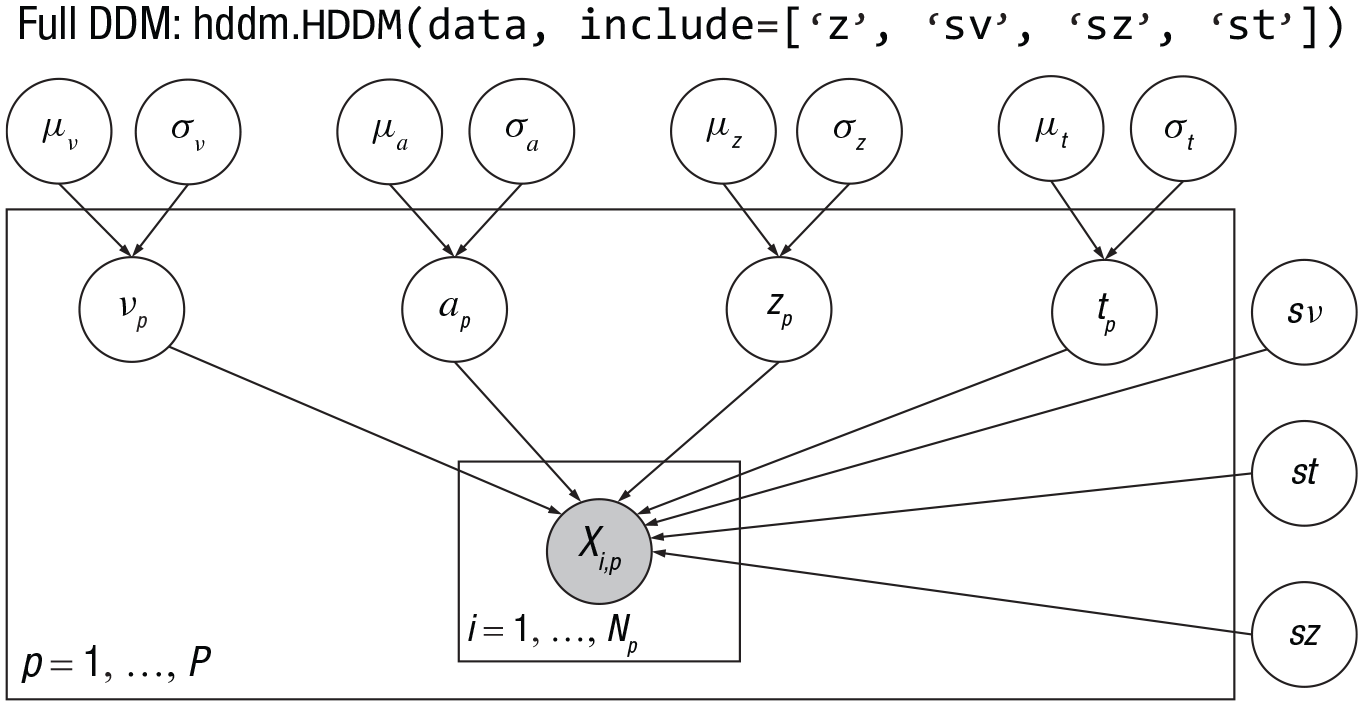
HDDM employs hierarchical Bayesian modeling by default, where each participant’s free parameters are sampled from population-level distributions (Wiecki et al., 2013). Taking full drift-diffusion model (DDM; Model 0) as an example, nondecision time t _p is assumed to be drawn from a normal distribution: t _p ~ N(μ _t ,σ _t ), where μ _t and σ _t are the mean and standard deviation of the population-level normal distribution of nondecision time t. Likewise, u _z /u _v /u _a and σ _z /σ _v /σ _a are the means and standard deviations for the other three parameters, respectively. In addition, three free parameters st/sv/sa indicate the trial-by-trial variability of nondecision time ( t ), drift rate ( v ), and initial bias ( a ), which are estimated only at the population level.

Note: The hierarchical structure of the full DDM in HDDM. The parameters inside and outside the rectangle are subject and population level parameters, respectively. p/i are the indices of participants (p=1, 2, …, p) and trials (i=1, 2, … N), where x_i,p is the data (choice/response time) of the ith trial in the pth subject.

Consequently, there are a total of 11 population-level parameters. At the subject level, subjects have their own estimate of the parameter of a, v, t, z, leading to a total of 4 × p subject-level parameters. Thus, in the full DDM, the number of parameters is 11 plus 4 × p.

HDDM provides two types of priors: weakly informative priors and noninformative priors. By default, dockerHDDM uses weakly informative priors as summarized in the table below (Wiecki et al., 2013). The default informative priors are suitable for most perceptual tasks. However, for tasks with longer response times, it is recommended to use noninformative priors. In this case, one has to set the parameter ‘informative=False’ when defining the model, for example, ‘m = hddm.HDDM(data, informative=False)’.

DDM parameters’ informative prior
μ v ~ $\mathcal{N}$ (2,3)	σ v ~ $\mathscr{H}\mathcal{N}$ (2)	v p ~ $\mathcal{N}({\mu }_v,{\sigma }_v^2)$
μ a $\mathcal{G}$ (1.5, 0.75)	σ a $\mathscr{H}\mathcal{N}$ (2)	a p $\mathcal{G}({\mu }_a,{\sigma }_a^2)$
μ z ~ invlogit ( $\mathcal{N}$ (0.5, 0.5))	σ z ~ $\mathscr{H}\mathcal{N}$ (0.05)	z p ~ $\mathcal{N}({\mu }_z,{\sigma }_z^2)$
μ t ~ $\mathcal{G}$ (0.4, 0.2)	σ t ~ $\mathscr{H}\mathcal{N}$ (1)	t p ~ $\mathcal{N}({\mu }_t,{\sigma }_t^2)$
sv ~ $\mathscr{H}\mathcal{N}$ (2)	st ~ $\mathscr{H}\mathcal{N}$ (0.3)	sz ~ $ℬ$ (1, 3)

Note: Table extracted and refined from Wiecki et al. (2013). $\mathcal{N}$ represents a normal distribution parameterized by the mean (μ) and standard deviation (σ). $\mathscr{H}\mathcal{N}$ represents a half-normal distribution, which is a positive-only distribution parameterized by the standard deviation. $\mathcal{G}$ represents a gamma distribution, parameterized by the mean (μ) and the rate (σ). β represents a beta distribution, parameterized by alpha and beta. The term invlogit represents the inverse logit function also known as the logistic function.

HDDM also allows parameters to vary with variables by integrating hierarchical linear regression models (also called “linear mixed models” or “multilevel models”). Specifically, the ‘hddm.HDDMRegressor()’ function allows any or all of the four parameters of DDM (a, v, t, z) to be modeled as a function of experimental conditions or other variables (e.g., EEG signal). In HDDM, the regression models are defined using the Python package patsy (see https://patsy.readthedocs.io/en/latest/quickstart.html), which uses the same syntax for defining regression functions as in other commonly used statistical packages. For example, in Model 2 in the main text, we used the expression ‘v ~ 1 + C(conf, Treatment(‘LC’))’, where the term to the left of “~” is the dependent variable and the term to the right of “~” is the regression equation. The term ‘1’ refers to the intercept, which corresponds to the variable “V_Intercept” in the output. The term “C(conf, Treatment(‘LC’))” indicates the slope coefficient, which corresponds to the variable “v_C(conf, Treatment(‘LC’))[T.HC]”. As in other hierarchical regression models, both the intercept and the slope can be estimated at the population level and the subject level (referred to as “fixed effects” and “random effects” or “varying effects,” respectively; D. J. Johnson et al., 2017; Pedersen & Frank, 2020; Wiecki et al., 2013), depending on how the model is specified. In ‘hddm.HDDMRegressor()’, the default is hierarchical model with random intercept but no random slope. We need to set ‘group_only_regressors=False’ to include the random slope (as we did in Model 2).

Although both the ‘depends_on’ argument and the ‘HDDMRegressor’ function allow parameters to vary with discrete variables (e.g., conflict levels), there is an important difference between them. The ‘depends_on’ argument defines the parameter split by condition. Specifically, the means of the parameters under each condition are derived from a share prior, whereas the variability of the parameters is consistent across conditions. The ‘HDDMRegressor’ function defines the relation between parameters and condition by a linear model specification, which means the intercept and slope in the linear regression both have their own priors. In a word, ‘depends_on’ is unable to use within-subjects effects because each subject’s condition is derived from the population prior, whereas ‘HDDMRegressor’ allows subjects to have their own intercept, which allows for the estimation of within-subjects variation across conditions. Thus, the choice of model definition is relevant to the assumptions made about the relationship between parameters and the experimental conditions. For more details, see Wiecki et al. (2013).

• Similarly in Box 4, the third and fourth paragraphs displayed incorrectly rendered symbols. The correct symbols are reflected below and updated online:

Box 4. Linking Deviance Information Criterion, Widely Applicable Information Criterion, and Pareto-Smoothed Importance Sampling Leave-One-Out Cross-Validation to Akaike Information Criterion

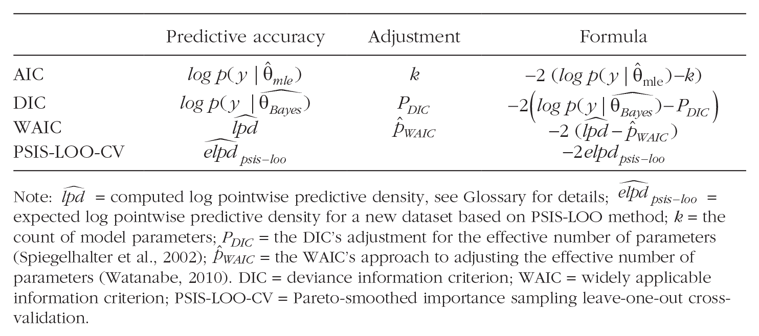
The deviance information criterion (DIC), widely applicable information criterion (WAIC), and Pareto-smoothed importance sampling leave-one-out cross-validation (PSIS-LOO-CV) are criteria founded on the concept of out-of-sample predictive accuracy, that is, the accuracy of using the fitted model to predict new data generated by the assumed data-generating process. Predictive accuracy is often encapsulated by the log predictive density (Box 1). However, the log predictive density approximated using the observed data and the posterior estimates of parameters is biased, and an adjustment is required to correct the bias. Thus, the key difference between DIC, WAIC, and PSIS-LOO-CV lies in the difference between the two terms of log predicted density and corrected bias (see the table below).

	Predictive accuracy	Adjustment	Formula
AIC	$logp(y|{\widehat{\mathrm{\theta }}}_{mle})$	k	$-2(logp(y|{\widehat{\mathrm{\theta }}}_{\mathrm{mle}})-k)$
DIC	$logp(y|\widehat{{\mathrm{\theta }}_{Bayes}})$	P DIC	$-2\left(logp(y|\widehat{{\mathrm{\theta }}_{Bayes}})-P_{DIC}\right)$
WAIC	$\widehat{lpd}$	${\widehat{p}}_{WAIC}$	$-2(\widehat{lpd}-{\widehat{p}}_{WAIC})$
PSIS-LOO-CV	${\widehat{elpd}}_{psis-loo}$		$-2elp{d}_{psis-loo}$

Note: $\widehat{lpd}$ = computed log pointwise predictive density, see Glossary for details; ${\widehat{elpd}}_{psis-loo}$ = expected log pointwise predictive density for a new dataset based on PSIS-LOO method; k = the count of model parameters; P _DIC = the DIC’s adjustment for the effective number of parameters (Spiegelhalter et al., 2002); ${\widehat{p}}_{WAIC}$ = the WAIC’s approach to adjusting the effective number of parameters (Watanabe, 2010). DIC = deviance information criterion; WAIC = widely applicable information criterion; PSIS-LOO-CV = Pareto-smoothed importance sampling leave-one-out cross-validation.

DIC uses the Bayesian posterior means for estimating log predictive density and includes an adjustment based on the effective number of parameters ( P _DIC ). It is particularly suited for hierarchical models, offering an improved estimate of predictive density (Spiegelhalter et al., 2002).

WAIC further refines DIC, evaluating the log predictive density across the entire posterior and correcting bias via the variability of log predictive density ( p̂ _WAIC ). This adjustment is crucial for measuring model robustness and guarding against overfitting (Watanabe, 2010). Both DIC and WAIC rely on estimating the effective number of parameters, but DIC assumes a Gaussian distribution for the likelihood, which simplifies the calculation (Lunn et al., 2012). In contrast, WAIC does not rely on this strict assumption and uses the full posterior distribution, offering greater flexibility and accuracy but at a higher computational complexity (Gelman et al., 2014).

PSIS-LOO-CV estimates the predictive density by simulating the leave-one-out cross-validation, which by definition is the out-of-sample predictive accuracy, so bias correction is no longer needed for PSIS-LOO-CV. For more details on these three indices, see Gelman et al. (2014) and Vehtari et al. (2017).

• In Figure 7, the caption has been corrected from “95% confidence interval” to “95% credible interval.”

Fig. 7.

(a) Statistical inference of parameters. The high-density interval (HDI; black line and texts) is compared with the region of practical equivalence (ROPE; red line and text). ‘var_names’ argument can be used to select both group-level and individual-level parameters for analysis. ‘hdi_prob’ argument specifies the probability of the HDI, typically set at 0.95 to correspond to a 95% credible interval. ‘rope’ defines the limitations of ROPE, which is a range considered to be equivalent to the null hypothesis or a reference value for the parameter. The results show no overlap between the 95% HDI and the ROPE, indicating that the parameter is credibly different from zero. (b) Violin plot of parameter posteriors at two conflict levels. The black line is the 95% HDI, and the white dot is the mean. The drift rate is lower in high-conflict (HC) conditions than in low-conflict (LC) conditions.

In addition, a few minor grammatical and typographical errors have been corrected throughout the article. All changes are now reflected in the current version of the article.