
Abstract
Recent studies in psychology have documented how analytic flexibility can result in different results from the same data set. Here, we demonstrate a package in the R programming language, DeclareDesign, that uses simulated data to diagnose the ways in which different analytic designs can give different outcomes. To illustrate features of the package, we contrast two analyses of a randomized controlled trial (RCT) of GraphoGame, an intervention to help children learn to read. The initial analysis found no evidence that the intervention was effective, but a subsequent reanalysis concluded that GraphoGame significantly improved children’s reading. With DeclareDesign, we can simulate data in which the truth is known and thus can identify which analysis is optimal for estimating the intervention effect using “diagnosands,” including bias, precision, and power. The simulations showed that the original analysis accurately estimated intervention effects, whereas selection of a subset of data in the reanalysis introduced substantial bias, overestimating the effect sizes. This problem was exacerbated by inclusion of multiple outcome measures in the reanalysis. Much has been written about the dangers of performing reanalyses of data from RCTs that violate the random assignment of participants to conditions; simulated data make this message clear and quantify the extent to which such practices introduce bias. The simulations confirm the original conclusion that the intervention has no benefit over “business as usual.” In this tutorial, we demonstrate several features of DeclareDesign, which can simulate observational and experimental research designs, allowing researchers to make principled decisions about which analysis to prefer.
There are several studies in the social sciences that show that different researchers analyzing the same data can come to different conclusions. One reason for discrepancies is unclear specification of the research question (Kummerfeld & Jones, 2023), but even when a question is clearly defined, differences can emerge because of analytic decisions (e.g., Schweinsberg et al., 2021). For example, Silberzahn et al. (2018) reported a study in which different analysts were given the same data concerning the rates at which light-skin-toned or dark-skin-toned soccer players were sent off the field by the referee. The research question was clear: Are referees more likely to send dark-skin-toned players off the field? With observational data such as these, there are many analytic decisions that might affect the outcome of the analyses. For example, should analyses control for the experience of the referee or the league which the player is in? The study found that different sets of analysts used different approaches that resulted in large differences in the effect size obtained. Such differences were not simply a product of the analysts’ experience. It seems that in the case of complex observational data such as these, it may be impossible to avoid differences in the outcome of analyses, depending on the covariates analysts choose to include in their model.
In this article, we focus on a potentially more straightforward issue: analyses of randomized experiments. Much has been written about the analysis of randomized trials (see Shadish et al., 2002). In the ideal case, a study is planned, participants are assigned randomly to treatments, and the analyses follow a preregistered plan to avoid the possible biases that may be introduced if analyses are changed after inspecting the data collected. There are two critical issues in the analysis of randomized studies. First, data should always be analyzed respecting the randomization; researchers should not “subvert” the randomization process by analyzing subgroups. Randomization ensures groups are balanced not just in terms of measured variables but also in terms of unknown confounders. This balance is destroyed if the randomization is broken. One issue that may compromise the conclusions that can be drawn from a randomized trial is attrition. If participants withdraw from a study, this potentially subverts the randomization process and can lead to misleading conclusions. More problematically, if post hoc subgroup analyses are performed, they need to be declared as exploratory, and such analyses cannot support causal conclusions about the intervention. Second, one needs to be aware of the dangers of adopting a flexible analytic pipeline if there are multiple outcome measures. Psychologists use the term “p-hacking” to refer to the problems that can arise if many analyses are conducted with only positive outcomes being reported without any recognition of how this can affect the probability of obtaining a “significant” result.
In summary, even in the case of randomized trials, in which typically the research question is well specified in advance and a preregistered analysis plan exists, complex issues of interpretation of analyses may arise because of attrition or failure of participants to comply with (receive) treatment or because a flexible approach to analysis is adopted that distorts the interpretation of p values. Although these issues have been recognized for years, these problems may be disregarded if researchers fail to appreciate the seriousness of the consequences of different analytic decisions. Our view is that it is important not just to exhort researchers to follow particular procedures but also to give them a sense of the extent of bias that can result if they fail to do so: For this purpose, simulation is a useful tool.
In this article, we describe DeclareDesign, a package in the R programming language that is designed to assess the effects of different analytic choices on outcomes from either observational or experimental studies such as randomized trials. DeclareDesign allows one to simulate data sets from specified designs and compare the effects of different sampling frames and analytic approaches (Blair et al., 2023; https://declaredesign.org/). DeclareDesign was developed in the field of political science but is not widely known outside that field despite its considerable benefits for researchers and policymakers. Simulations allow researchers to create data sets in which the true values of estimated parameters are known and then see how well those values are recovered in an analysis. In particular, as well as checking whether a design is suitable for minimizing the rate of false negatives (i.e., has adequate power), one can estimate the likelihood of false-positive findings (i.e., bias).
DeclareDesign adopts a formal approach to research design, distinguishing between four steps—model, inquiry, data strategy, and answer strategy—that are combined to characterize a design that can then be evaluated using simulated data. Blair et al. (2019) noted that although simulated data are often used to estimate the statistical power of a design, they are seldom used to evaluate other properties of interest, known as “diagnosands,” such as precision of estimates (as reflected in the root mean square error [RMSE]), and bias (systematic differences between estimates and true values). Another index, coverage, combines aspects of precision and bias, reflecting the probability that the confidence interval around an estimate contains the true value. Practical diagnosands, such as cost of a study, can also be included. A useful feature of the package is that once a research design has been specified, it is easy to manipulate parameters to see their effect on statistical power, precision, bias, and other diagnosands for a proposed study. It has a modular structure that also makes it easy to create new designs by combining features of old designs.
Background to the Tutorial
In this tutorial, we introduce DeclareDesign with a worked example. To follow the tutorial, readers will need to be familiar with analyzing regression models using the programming language R.
To illustrate how DeclareDesign can be used to compare different approaches to analyzing data from an intervention trial, we take as a case study a large randomized controlled trial (RCT) that evaluated the effectiveness of GraphoGame (GG) Rime (https://graphogame.com), a computer-based game designed to improve children’s reading (see Goswami & East, 2000). This example is pertinent because there are published analyses of the RCT that come to contradictory conclusions.
The GG RCT was funded jointly by the Wellcome Trust and the Education Endowment Foundation (EEF) as part of a scheme to develop collaborative intervention research between educators and neuroscientists. This trial, registered at http://www.isrctn.com/ISRCTN10467450, selected poor readers who were randomly assigned within classrooms to GG Rime or a business-as-usual control group. To minimize possible bias from experimenters’ conflict of interest, EEF projects undergo independent evaluation by researchers who are not involved in obtaining the funding. Details of the original RCT are provided in the report by independent evaluators from the National Foundation for Educational Research (NFER; Worth et al., 2018). The conclusion from this independently conducted evaluation was stark: “The trial found no evidence that GG Rime improves pupils’ reading or spelling test scores when compared with business-as-usual. This result has very high security.” The high-security rating refers to the EEF’s rating of the methodological quality of this randomized trial. A reanalysis was conducted by researchers at the University of Cambridge, who had developed the English version of GG Rime and had obtained the funding for the study. The Cambridge analysis concluded that “the current study suggests that young learners of the English orthography show significant benefits in learning both phonic decoding skills and spelling skills from the supplementary use of GG Rime in addition to ongoing classroom literacy instruction” (Ahmed et al., 2020). Individuals considering using GG will find it confusing that such diametrically opposed conclusions can be drawn from analysis of the same data set. Here, we show how modeling the contrasting analytic approaches clarifies the sources of disagreement.
Method
We simulated six different designs to illustrate the impact of different analytic choices using the DeclareDesign package (Blair et al., 2023) in the R computing language (R Core Team, 2023). The simulated designs demonstrated the impact of five features of the designs used by the NFER and Cambridge groups.
Basic pretest–posttest design with variable correlation between pretest and posttest (outcome) measures
The NFER analysis used a preregistered outcome measure: the score on the New Group Reading Test (NGRT). On the basis of earlier research, Worth et al. (2018) did a power analysis based on an anticipated pretest–posttest correlation of .8. They did not explain their power analysis in detail, but in their protocol, they stated that with a sample size of 400, they would be able to detect an effect size of 0.17 (presumably Cohen’s d) with 80% power and that attrition of 10% would still yield a minimum detectable effect size of 0.18 at 80% power. In practice, the observed pretest–posttest correlation on the NGRT was lower (.57) than the value used in the power calculations, so the power of the study to detect a genuine effect was reduced. In Design 1, we introduce DeclareDesign with the basic design used by the NFER evaluators and show how simulations can be generated to diagnose the properties of the design; in particular, we quantify the impact of pretest–posttest correlation on the power of the design to estimate the intervention effect.
Control for clustering by classroom
The NFER analysis included a term in the regression analysis that took into account clustering of scores by classroom. This was not done in the Cambridge analysis. With Design 2, we show how to modify Design 1 to simulate data that are hierarchically clustered and see how this affects diagnosands.
Analysis of covariance (regression) versus repeated measures analysis of variance
The Cambridge reanalysis treated pretest and posttest reading scores as two levels of a dependent variable in repeated measures analysis of variance (ANOVA), whereas in the original NFER analysis, regression was used with posttest score as the outcome and pretest as a covariate. In Design 3, we incorporate a comparison of diagnosands from these two analytic approaches.
Use of multiple outcomes
The NFER analysis focused on a single preregistered outcome measure. The Cambridge reanalysis took results from five related outcome measures. In Design 4, we simulate five correlated measures given at pretest and posttest and model the impact of p-hacking.
Selection of participants for analysis
The NFER analysis included all participants in the RCT for whom outcome data were available. The Cambridge reanalysis dropped half of the intervention group, who were below average in the level of the game they had achieved, on the grounds that they may not have been engaged with the intervention. In Design 5, we consider the consequences of modifying Design 1 to restrict analysis to a subset of participants from the intervention group.
Combining Designs 4 and 5
In Design 6, we considered the effect of combining Designs 4 and 5 to model the Cambridge reanalysis as closely as possible.
For each analysis, we considered the diagnosands statistical power, bias, RMSE, and coverage.
Design 1: Simulation of Original Analysis With Variable Correlations Between Pretest and Posttest Measures
We started by simulating data from the original trial, which adopted a standard approach for analyzing an RCT (Shadish et al., 2002) in which children were randomly assigned to intervention or control groups. As is typical in education research, the control group included children receiving usual classroom education—a so-called business-as-usual control group. The GG intervention was compared with business as usual in a sample of 398 Year 2 pupils from 15 primary schools. All participants were selected as having low literacy skills, as assessed by the phonics screening check, a national assessment that is taken at the end of Year 1, when children are around 6 years old. GG training occurred during literacy sessions, when the control group children received regular literacy activities with the class teacher. This was a two-armed pupil-randomized controlled trial powered for a minimal detectable effect size (Cohen’s d or standardized mean difference) of 0.17. Final data were available for 362 children from two cohorts, each of which did the intervention for one spring term in successive years. Allocation to intervention or control group was done by stratified random assignment of pupils within classroom to ensure roughly equal numbers of children in intervention and control groups in each classroom. Worth et al. (2018) noted that attrition was around 10% for both intervention and control groups and did not appear biased but, rather, was due to chance events, such as absence on the day of the test. Analysis of covariance (ANCOVA; regression) was used to estimate the effects of the intervention on a preregistered outcome measure, with a pretest score used as a covariate.
The DeclareDesign package includes a Design Library, with R code for simulating common experimental designs (see https://declaredesign.org/r/designlibrary/). We took as our starting point the pretest–posttest design (https://declaredesign.org/r/designlibrary/articles/pretest_posttest.html), which implements the type of analysis used by NFER. Although the design can be evaluated in a single step with specified parameters, we walk through the model, inquiry, data strategy, and answer strategy separately to clarify the modular approach used in DeclareDesign. Much of the strength of DeclareDesign comes from this modularity; as we show, once one has declared an initial design, it is straightforward to use elements of that design in a new design. We include code chunks here to illustrate the key features of DeclareDesign. For the full code for all computations used in this article, see the Supplemental Material available online.
Model
To simulate data from a study, one needs to specify which variables to simulate, how they are generated, and the relationships between variables. This specification corresponds to the theoretical part of the design, referred to as the “model.” For the pretest–posttest experiment, one needs to specify the underlying distribution of the data, the correlation between pretest and posttest scores, and the effect size of the intervention.
The code chunk DESIGN 1: MODEL SPECIFICATION below illustrates how the model is coded for the pretest-posttest design. A potentially confusing feature of DeclareDesign is that the various “declare” functions do not compute results but, rather, specify new functions. These functions are then combined to create a full design specification. The order of functions is crucial because each function takes as its input the output of the prior function. In this tutorial, we have added steps that compute the results of functions; these serve a purely didactic purpose in making explicit what the function does and allow users to check that the model specified behaves as expected.
A second potential source of confusion is that DeclareDesign distinguishes between unobserved latent values and observed values. In the context of the pretest–posttest design used here, for each simulated participant, we simulate a value of U (unobserved value) at Time 1. The expected outcome at Time 2 is represented by Y and will depend on U and on the intervention condition, Z.
For didactic purposes, we have added some additional steps to the code to make it possible to inspect results of the different steps; in addition, some variable names have been changed to make them more aligned with terminology commonly used in psychology.
For simplicity, we simulate scores as normally distributed with a standard deviation of 1, although virtually any kind of statistical distribution can be simulated. One needs to specify the sample size (before attrition), N; the correlation between pretest and posttest scores, rho; and the size of the intervention effect, or EffSize (in the DeclareDesign examples, this is referred to as “ate” or “Average Treatment Effect”). Our simulated data start as z scores, with mean of 0 and standard deviation of 1, and so EffSize (difference in means for treatment vs. control groups) is the same as the standardized mean difference, also known as Cohen’s d (difference in means divided by pooled standard deviation).
Our model includes one term that is not part of the DeclareDesign pretest–posttest example: improvement from Time 1 to Time 2 regardless of intervention. Our example concerns children learning to read, and children’s scores will improve just because of factors such as maturation or practice on the tests. The NFER analysis reported general improvement in scores on the reading test from Time 1 to Time 2 of around 1 SD regardless of intervention, so we specified a further term, “gain_t1t2,” which is added to Time 2 scores.

For the first eight rows of the resulting simulated data, see Table 1.
Simulated Potential Outcomes for Design 1

The first function, population, generates the first four columns for 398 rows. The first column, ID, identifies each simulated participant by a sequential number. Columns with the prefix “u_” correspond to unobserved latent variables; u_t1 represents Time 1 scores, and u_t2 represents Time 2 scores. The code specifies that these are drawn from a population in which u_t1 and u_t2 are correlated with correlation rho. For the whole data frame, the mean of u_t2 is greater than u_t1 by the value gain_t1t2. Note that the inclusion of the “gain_t1t2” term has no impact on the estimate of the intervention effect size because it applies regardless of intervention status. It is included here just to ensure that the simulated data resemble real data in terms of giving higher scores at Time 2 than Time 1.
Columns with the prefix “Y_” correspond to expected values for observed variables. Y_t1 is equal to u_t1 and corresponds to the observed pretest value. Although this is redundant, it clarifies the distinction between unobserved, latent variables and observed variables. For Y_t2, there are two values generated, Y_t2_Z_0 and Y_t2_Z_1. These are the expected observed values at posttest (potential outcomes), depending on whether the case is allocated to the control group (Z_0) or the intervention group (Z_1). The values of Y_t2_Z_0 are the same as values of u_t2, whereas the values of Y_t2_Z_1 correspond to u_t2 plus the value of EffSize. That is, Y_t2_Z_1 corresponds to the expected observed value at posttest plus an added component equal to the average treatment effect. Note that the individual variation in outcomes arises from u_t2; the average treatment effect is constant.
Inquiry
The inquiry specifies what parameter one wants to estimate from the design—known as the “estimand.” This could be a descriptive statistic, such as the mean value of a variable or the difference or correlation between variables. Here, we specify the estimand as the mean difference between intervention and control groups at Time 2, that is, the average treatment effect.

If we apply the estimand function to the data frame generated at the model stage, we get a value of the estimand of 0. Although this is reassuring, it is hardly surprising because we defined Y_t2_Z_0 and Y_t2_Z_1 as equivalent and specified EffSize as zero, which was to be added to the Y_t2_Z_1 condition. In subsequent steps, we consider how the estimand compares with estimates of its value in subsets of simulated data, where we vary the EffSize. Differences between the estimand and estimates indicate how much bias there is in the analysis.
Data strategy
The data strategy selects data for allocation to treatments and for analysis. In the chunks of code below, we first use “declare_assignment” to randomly assign cases to Z = 0 (control) or Z = 1 (intervention) and then use it again to specify whether the case HasData (using the attrition rate to randomly assign a proportion of cases as HasData = 0). We also make a new column that shows the outcome corresponding to the intervention assignment for each case, and finally, we compute the observed difference (diff_t1t2) between posttest and pretest scores for each row.

For the first eight rows of resulting simulated data from this code, see Table 2.
Simulated Data With Assignment to Intervention for Design 1

When all steps of the data strategy are complete, the simulated data frame now has additional columns. Column Z indicates whether the individual is assigned to control (0) or intervention (1) condition. HasData is 1 for most cases and 0 for around 9%. The Y_t2 column is created by selecting Y_t2_Z_0 where Z is 0 and Y_t2_Z_1 where Z is 1. The final column is the observed difference between scores at Time 2 and Time 1. The latter is not used for our current analysis but will feature in Model 3. Note that values of outcome (Time 2) variables are computed even when HasData = 0. We exclude these values from the analysis at the next step.
Answer strategy
The answer strategy involves first fitting a statistical model to data and then summarizing the model fit.
We use “declare_estimator” to indicate which statistical analysis to conduct and to link this to our estimand. The example of the “pretest_posttest” function in the DeclareDesign vignette compares three different analytic approaches, all implemented in linear models. For now, we focus just on an analysis in which we compare outcome scores (Y_t2) for the two treatment groups (Z) using pretest score (Y_t1) as a covariate. This is a recommended approach for analysis of RCTs, and in a standard analysis, it would be achieved by a command such as “lm (Y_t2 ~ Z + Y_t1).”
In DeclareDesign, we use the declare_estimator function, specifying the “.method = lm_robust”; this fits an ordinary least squares linear model and formats the output summary. Note that at this stage, we can also specify which cases are included with the code “subset = HasData ==1.”

Again, we save the output into a table just for didactic purposes to show what the declare_estimator step achieves.
Table 3 shows the effect of running the “myancova” function on a single simulated data set. The “statistic” here is a t value that tests the statistical significance of the prediction of outcome from a dummy code (Z) representing intervention after controlling for pretest score. The output is the same as for the following code:

Output From Linear Regression Applied to One Run of Simulated Data

To get a reliable estimate of the properties of this design and the variability around the estimated parameters, we need to run the simulation many times. We first create our full design by bolting together the elements of the model, inquiry, data strategy, and answer strategy and then run “diagnose_design” with a specified number of simulations. We can also use the “redesign” function to change the values of parameters and rerun the simulation to see the effect. Here, we compare results when the true effect size is 0 with the same design when the true effect size is .2. In addition, we consider how varying the correlation between the pretest measure and posttest measure affects results by comparing results when the correlation, rho, is set to .6 versus .8. This is pertinent to the current example given that the test-retest correlation for the outcome measure used by NFER was lower than predicted.

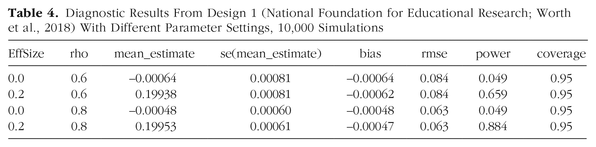
The default output from the model diagnosis (saved in “Design1_diagnosis$diagnosands_df”) has more detail than we need, and we present here simplified tables that show just the parameters varied in the design, the mean estimate of intervention effect with its standard error, the bias (i.e., mean estimate minus estimand), RMSE, the statistical power, and the coverage (probability that the confidence interval contains the true value). An optimal design will give estimates close to the true value (estimand), with RMSE below .1 and coverage around .95. The proportion of significant estimates is labeled as “power.” In cases in which the true effect size is greater than zero, power indicates the probability of detecting a genuine effect given the research design. If, however, the true effect size is zero, then this value corresponds to the false-positive rate and is expected to be close to the specified alpha (.05 in this case): The estimate here is 0.049. Where rho = .6, power is low (66%) to detect an effect size (Cohen’s d or standardized mean difference between groups) of 0.2. In contrast, where rho = .8, power is increased substantially (88% power to detect an effect size of 0.2).
When we run “diagnose_designs,” we create a structure that saves the result from each simulation in a data frame and a data frame containing the diagnosands for each set of parameters. These can be used for generating graphical displays of results.
Figure 1 shows graphically the distribution of estimates from the model after 10,000 runs of each simulation with four different parameter settings (two values of rho and effect sizes of 0 or 0.2).
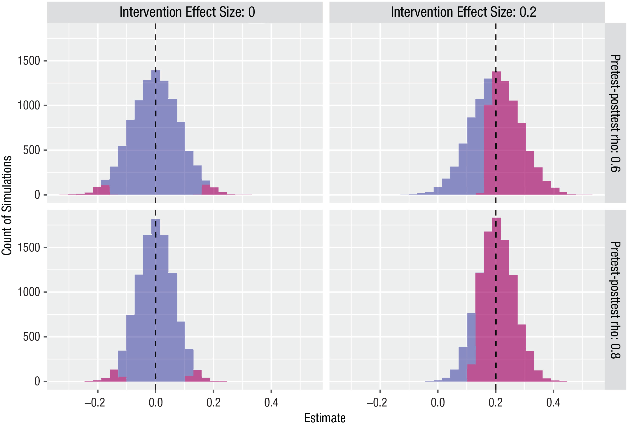
Simulated distributions of estimated effect size for Design 1, 10,000 simulations. The blue corresponds to nonsignificant estimates, and the purple corresponds to estimates where p < .05. For the null case, in which the true intervention effect size is zero, the purple regions correspond to false positives on a two-tailed test. Dashed vertical line shows true effect size.
Figure 1 illustrates two features of the designs. First, the simulated data generate the “true” effect sizes accurately (mean effect sizes of 0.0 and 0.2 as expected). Second, an increase in the pretest–posttest correlation does not affect the estimated effect size, but variability in the estimates of the effect size is smaller (i.e., the standard errors of the estimates are lower) when the correlation is higher, leading to higher power to detect a true effect.
Design 2: Modifying the Simulation to Incorporate Classroom as a Cluster
Note that research designs that involve clustering are more complicated than other designs considered here. Here, we show how to model a clustered design, but the conclusion is that in the design used by the GG study, clustering has no impact on bias or power and can be ignored. We present the full analysis here for completeness, but readers can skip to Design 3 without any loss of continuity.
Analyses of intervention studies conducted in schools can be affected by clustering if randomization is conducted at the level of schools or classrooms because children within a school/classroom are likely to be more similar to each other than to children from different schools/classrooms. Standard errors and p values from a typical regression model depend on the assumption that the residuals in the model across cases are independent from each other. If children within classrooms are more similar to each other, the assumption of the independence of residuals is violated, and this will usually reduce the precision of confidence intervals (and hence reduce the statistical significance of effects).
Children from 53 classrooms were included in the GG trial, with an average of 7.5 pupils per class eligible for the trial, who were randomly assigned within classrooms to either receive or not receive the intervention. Random assignment within classrooms in the trial means that estimates of the intervention effect should not be affected by clustering within classrooms, but for completeness, here, we explain how the effects of different ways of handling clustering in the data can be modeled.
Modeling clustered data is complicated for two reasons. First, at the model-specification stage, we need to incorporate the clustering into our simulated data. Second, at the answer-strategy step, we need to specify how to handle the clustering.
We start by modifying the model specification to introduce clustering by classroom. The key statistic for any analysis that seeks to control for the effects of clusters is the intracluster correlation (ICC). The ICC is the proportion of total variance in a dependent variable explained by the cluster variable. So, an ICC of .15 means that 15% of the variance in scores can be explained by the cluster variable. Typically, ICCs greater than .10 are considered likely to have significant effects on standard errors. There are various estimators for the ICC, but in this case, we use an estimator from the fishmethods() package based on a random-effects ANOVA model.

The inquiry is the same as for Design 1, but the data strategy needs modifying to take clustering into account. DeclareDesign offers different options for dealing with clusters in the analysis. One option is to randomize intervention assignment within class—this was done in the NFER analysis and can be achieved with the “strata_rs” command. DeclareDesign has another option for handling clusters, which is to randomize by cluster using the “cluster_rs” command. For instance, the 53 classrooms in the study could each be randomized to either intervention or control, with all children in the classroom treated the same. We mention this here to illustrate the flexibility of DeclareDesign but will not consider randomization by cluster further because it requires a different analysis strategy (see Blair et al., 2023, Chapter 18).

We need to modify the answer strategy to take clustering into account. There is much debate among methodologists about the best way to take such effects into account. The “.method = lm_robust” syntax in the answer strategy allows us to specify one of a variety of methods for dealing with the effects of clustering on standard errors (for details, see R. Bell & McCaffrey, 2002). In the code chunk below, class is designated as a cluster and included as a fixed effect, following the approach adopted in the NFER analysis. Given that in this case we have specified “cluster = class” without any options, this yields standard errors based on the HC2 variance estimator, first proposed by MacKinnon and White (1985). Other options are available, including the HC1 variance estimator as implemented in Stata, which is usually referred to as the “Huber-White sandwich estimator.” In practice, all of these different estimators try to correct for inaccuracies in standard errors that arise from violations of the assumption of independence of the residuals in the regression model because of clustering. In a case such as this, in which the ICC is small, different methods are unlikely to yield substantially different standard errors, and details of the methods are not relevant here. However, in cases in which the ICC is substantial in a cluster randomized design, these various methods will typically result in larger standard errors (and hence less significant p values) than nonclustered standard errors. If one were uncertain about the appropriate analysis, it would be easy in DeclareDesign to modify the code to adopt a different method and test its effect.
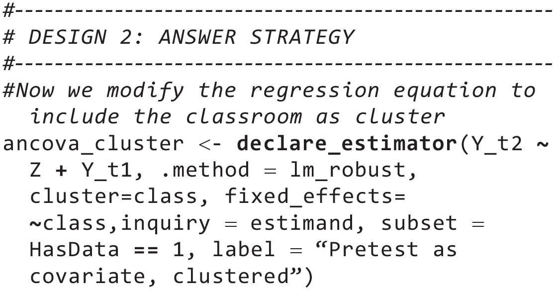
The design declaration is the same as for Design 1 except we substitute “classmodel” and “popmodel” in the model, use “assignment1” to randomly assign within class, and use “ancova_cluster” in the answer strategy.

A final point to note is that our model simulation specifies an ICC based on pretest data, whereas in intervention trials, it is the ICC for posttest data that is typically reported. When we simulate data in DeclareDesign, we start with the model for preintervention data and then add the intervention effect to create postintervention outcomes. Any clustering does not occur at the point of outcomes but is, rather, carried over from clustering in the preintervention model. Therefore, it does not make sense to simulate data in which clustering is seen only in posttest data. However, unless there is a very high correlation between pretest and posttest data (rho), the ICC for pretest data will be higher than that in posttest data. So, a final challenge is to estimate an appropriate ICC to use in the simulation, assuming that we know the ICC for posttest data, but for the model stage, we need to specify the ICC for pretest data. To do this, we ran a separate simulation to create a lookup table, “ICCmultiplier.csv.” This gives estimates for a multiplication factor to convert values of ICCpost into ICCpre for a given rho. For instance, when rho is .6, the corresponding values for ICCpretest is nearly 3 times greater than ICCposttest. The supplementary file “MakeICCMultiplier.Rmd” contains the code for creating the lookup table and is available on OSF (https://osf.io/jeprq/).
The results in Table 4 confirm that the clustering by classroom has a negligible effect on the analysis even when the ICC for classroom is relatively high. In this case, because children were randomly assigned within classrooms, including classroom as a cluster variable in the analysis has no effect on statistical power. If this had been a cluster-randomized design in which randomization was at the classroom level, the higher the ICC, the lower the power would be. Given that the ICC does not affect power here, for Models 3 through 5, we ignore the effect of clusters.
Diagnostic Results From Design 1 (National Foundation for Educational Research; Worth et al., 2018) With Different Parameter Settings, 10,000 Simulations
Design 3: Comparing Repeated Measures ANOVA With ANCOVA
The Cambridge reanalysis treated pretest and posttest scores as different levels of a dependent variable in an ANOVA in which group was the between-subjects factor and time was the within-subjects factor. The intervention effect was then estimated from the interaction term. Mathematically, this is equivalent to t test comparing the pretest/posttest difference scores for the intervention group versus the control group (the Time 2 score minus the Time 1 score for each participant in the two groups). We can readily check the impact of this analytic decision using code that is included in the “pretest_posttest” function in the DeclareDesign vignette. (https://declaredesign.org/r/designlibrary/articles/pretest_posttest.html). This time, our design includes two alternative analyses of the same simulated data—the original regression with pretest as covariate from Design 1 and the analysis of difference scores. Note that once the design is set up, it is trivially easy to incorporate this additional comparison in DeclareDesign. The model, inquiry, and data strategy are unchanged from Design 1; we add a new term just to the answer strategy.

The declaration of the design is identical to Design 1 except that we now include two different answer strategies: the original “myancova” (ANCOVA) and the new “changescore” (repeated measures ANOVA). Our diagnosis will then show both methods compared using the same simulated data.

The summary in Table 5 confirms that precision is greater (i.e., lower RMSE) and power is higher for the ANCOVA analysis than for the repeated measures ANOVA when there is a true intervention effect, although these differences are relatively small. The ANCOVA model is preferred because it has higher power and it better accounts for the correlation between pretest and posttest scores than using simple difference scores. In subsequent models, we use the ANCOVA analysis.
Comparison of Analysis of Covariance (Regression) Versus Repeated Measures (Change Score) Analysis

Design 4: Including Multiple Outcomes
The Cambridge group had administered some additional measures to participating children: Two subtests from the Test of Word Reading Efficiency (TOWRE) were given at follow-up and again at Time 3, after a delay. They reported analyses of five outcome measures (NGRT, TOWRE word, TOWRE nonword at posttest, TOWRE word, and TOWRE nonword at delayed posttest). Of these five analyses, just one showed a significant effect of intervention: a significantly larger improvement in the GG group on the TOWRE nonword subtest (p = .027) at immediate posttest. Neither of the TOWRE subtests differed between the intervention and control groups at the delayed subtest after the school summer holiday. No adjustment for multiple comparisons was made.
It is well established that false positives will increase if several outcomes are analyzed without any statistical correction for multiple comparisons (Lawson et al., 2021). Nevertheless, the standard recommendation to have a single outcome measure is not necessarily optimal in educational trials, in which there may be a range of outcome measures that might be expected to be influenced by the intervention (Bishop, 2023). It is not unusual for multiple correlated outcomes to be tested, and typically, they are different measures of the same underlying construct—in this case, literacy development. Here, we show how DeclareDesign can be used to diagnose properties of the design when there are correlated outcome measures.
To generate measures in the simulation, we first create a correlation matrix for five measures. In theory, it would be possible to use the correlation matrix from the original RCT data set, but this was not made available to us. Accordingly, we simulated five measures taken at both pretest and posttest, specifying plausible estimates for these based on our experience with comparable tests. The test-retest correlation for each measure was set at .7, the intercorrelation between different measures taken on the same occasion was set at .6, and the intercorrelation between different measures on different occasions was set at .4. Note that the “redesign” feature of DeclareDesign gives flexibility to alter these estimates of correlations and consider the consequences.
We also included a correlation of .2 between all measures and a “Level” index, which we explain in Design 6 but for now can be ignored. We use the “draw_multivariate” function of DeclareDesign, which uses the “mvrnorm” function from the MASS package in R to generate data with the specified correlations. Note that the specified correlations have to be in a realistic range. If, for instance, you have three variables, A, B, and C, and you specified that variables A and B were correlated .9 and that A and C were correlated .1, then the function would give an error message (nonpositive definite correlation matrix) if you specified that B and C were correlated .9 because it is just not possible to select variables to conform to these constraints.

The code for model, inquiry, data strategy, and answer strategy for Design 4 from this point is equivalent to that for Design 1 except that we create potential outcomes, estimands, observed outcomes, and estimators separately for each of the five outcome variables (for the full code, see the Supplemental Material).
We then specify Design 4, which includes all five variables (here labeled as “a,” “b,” “c,” “d,” and “e”).

For this model, if we just look at the diagnosand data frame from Design4_Diagnosis, we find diagnosands that are similar to those in Design 1 because each individual outcome behaves like a single outcome. The multiple outcomes, however, introduce potential for an increase in the false-positive rate through what is known as p-hacking—a case in which a researcher selects any of the set of outcome measures as evidence for effectiveness. The greater the number of measures, the more opportunities are for finding a significant result even when the true effect size is zero.
When modeling this situation, we have to decide what kind of selection might be made. Potentially, the researcher might be interested in any result that is statistically significant. However, that seems implausible because it would include negative and positive results. In our simulation, we simulate p-hacking by assuming that the researcher selects the largest positive effect size and disregards results that are opposite to prediction. We create a “p.hack” function, which uses the simulations that are stored as part of “Design4_diagnosis,” and for each run, we select the variable giving the most extreme positive result.

The first 12 rows of simulation results selected by the “p.hack” function are shown in Table 6 for the case in which the null hypothesis is true (EffSize = 0). The inquiry indicates which of the five measures, a, b, c, d, or e, was selected as most extreme. If the five measures were uncorrelated, then each measure would have an independent probability of showing a positive “significant” effect (p < .05) of .025 and a corresponding probability of a null result of .975. The chance of obtaining null results on all of the five tests is .975^5, which is equal to 0.88, and correspondingly, the chance of a false positive on at least one of the five tests is 1 – .975^5, which is equivalent to 0.12. However, the more highly correlated the outcome measures are, the less the false-positive rate will be inflated. We can categorize the p value of the most positive result on each run as either 1 (i.e., significant at p < .05) or 0 (nonsignificant) to compute the false-positive rate after p-hacking. For outcomes with the correlation structure used here, with significance counted only for effects in which the effect size is positive, the probability of a false positive (i.e., a positive estimate with a p value below .05 on at least one of five measures) is 0.08 when the true effect size is zero. Thus, in this case, running five separate statistical tests on a set of correlated outcome measures yields a small increase in the probability of falsely concluding that an effect exists when in fact, there is no true effect. The simulation therefore supports the well-established conclusion that performing multiple tests on the same data will increase the probability of finding false positives (erroneously finding support for a hypothesis when no true effect exists). DeclareDesign quantifies this effect and in this case, shows that the effect of multiple comparisons, on its own, is relatively small.
Most Extreme Positive Results From the First 12 Simulations of Design 4

Design 5: Modifying the Selection of Cases to Match the Cambridge Analyses
The Cambridge group reanalyzed the data after dropping children from the intervention group who had not progressed beyond the mean level achieved on GG for the whole intervention group. These 95 intervention cases were then compared with the whole control group on a range of outcome measures. The rationale for this approach is that playing time was very variable, and some children may have used their time alone on the computer to do other activities. It was argued that it would be a fairer test to restrict consideration to children who had progressed far enough through the game to indicate that they had “received sufficient independent and solitary exposure to the game to learn English phonics” (Ahmed et al., 2020, p. 4).
As discussed briefly in the introduction, this analysis strategy is flawed and likely to introduce bias because it violates the random allocation of participants to groups. In this case, the Cambridge analyses compared children who performed well on GG (i.e., children who were learning to read well during the time in the study) with the whole of the control group (i.e., a group of children including many who would not be expected to learn to read well). This approach is similar to what is called a “per protocol analysis” in clinical trials in which patients in the intervention group who completed the treatment are compared with the control group. Per protocol analysis introduces bias because the characteristics of the intervention group in terms of known and unknown risk factors relevant to response to treatment are no longer matched to those in the control group by random assignment. The approach taken by the Cambridge group is actually more likely than a per protocol analysis to introduce bias because selection of children was not done based on whether children had played the game but, rather, on progress on GG (i.e., based on response to treatment, not whether treatment had been received).
In fact, it is already known from the NFER report that more time playing GG was not in itself associated with better progress in reading. In the NFER report, Worth et al. (2018) reported a negative correlation between the amount of time spent playing GG and reading posttest scores (r = –.298): That is, the more time the child spent playing the game, the less progress they made. Instead, the Cambridge group took the subset of children who made the most progress through the game. The game is adaptive, progressing through 25 streams of phonic knowledge, and children move on to a higher stream only if they have reached a satisfactory level on a lower stream. The mean point reached by all the intervention group was Level 5 of Stream 16. So, the authors selected a “top half” group of children who progressed beyond that point. We refer to this as the “top-half” GG group. This is a group of children who, based on their progress on GG, are mastering the rules of phonics better than the other children in the intervention group.
It is straightforward to modify Design 1 to represent the selection of the top-half GG cases as was done in the Cambridge analysis. To do this, we create a new latent variable, level, which represents the level reached by players of GG. This is modeled as a random normal deviate, as for the other latent variables. A critical issue is how far it correlates with u_t2 (the level of the unobserved latent reading ability at Time 2). We can model this scenario with a new variable, r_L.u2, which represents the correlation between the level reached on GG and u_t2 (the unobserved latent reading ability at Time 2). It seems likely that the children who progress furthest through the game are the children that learn fastest on GG, which after all, is a measure of learning to read (learning correspondences between letters and groups of letters in printed words and their pronunciations). Thus, we anticipate that r_L.u2 will be greater than zero.

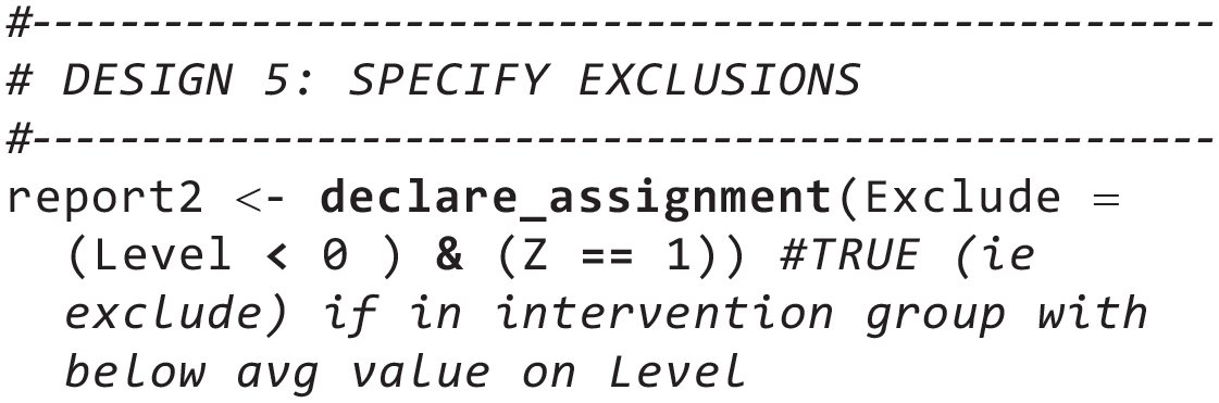
We next need to add a new “declare_assignment” step to the data strategy that selects which participants will be excluded. Because level is a random normal deviate and children are excluded if they are below average on the level variable, then we can just exclude children in the intervention group who have a value of level below zero.
Finally, we need to modify the Answer Strategy to incorporate the new exclusion. We name this new answer ancova_sel, to denote that it is an ANCOVA with selection
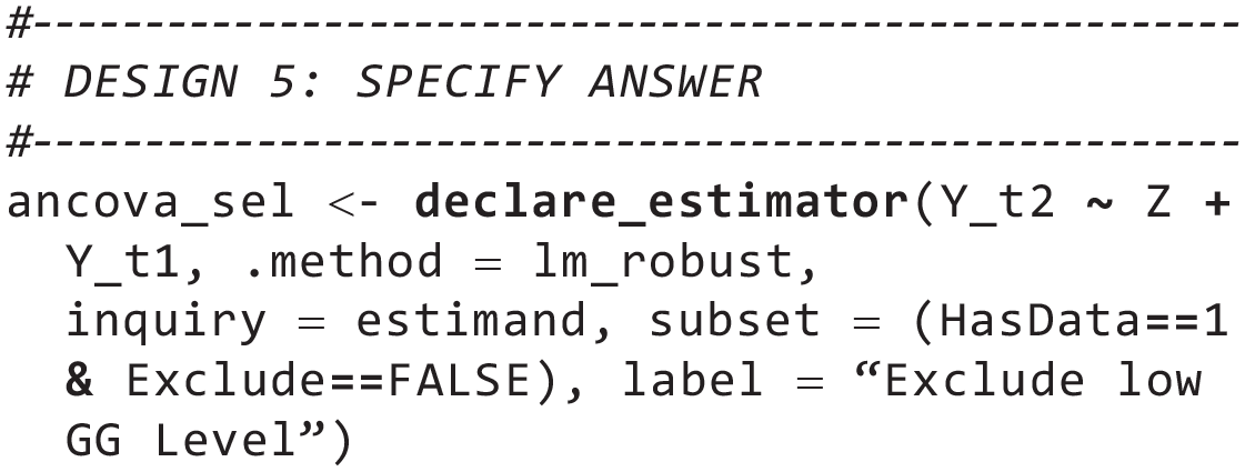
The Design 5 declaration differs from Design 1 in terms of the initial “population_sel” declaration; in the inclusion of the “report2” declaration, which defines the exclusion criteria; and in the use of “ancova_sel” in the answer. All other declarations are carried over from Design 1.

Table 7 shows that the selection of cases based on level creates upwardly biased estimates of the intervention effect when level is correlated with the outcome measures (i.e., when r_L.u2 is greater than zero). When the null hypothesis is true, the estimates of effect size are 0.1 and 0.21 if correlation with the selection measure is .2 or .4, respectively. Note that when the null is true, then “power” indicates the false-positive rate, which should be around .05. The simulated data give values of power (i.e., estimates of the rate of falsely producing evidence of an effect when no effect exists) of .17 and .53 when the correlation with selection variable is .2 or .4, respectively.
Diagnostic Results From Design 5 at Two Effect Sizes, With Different Correlations Between Level and u_t2
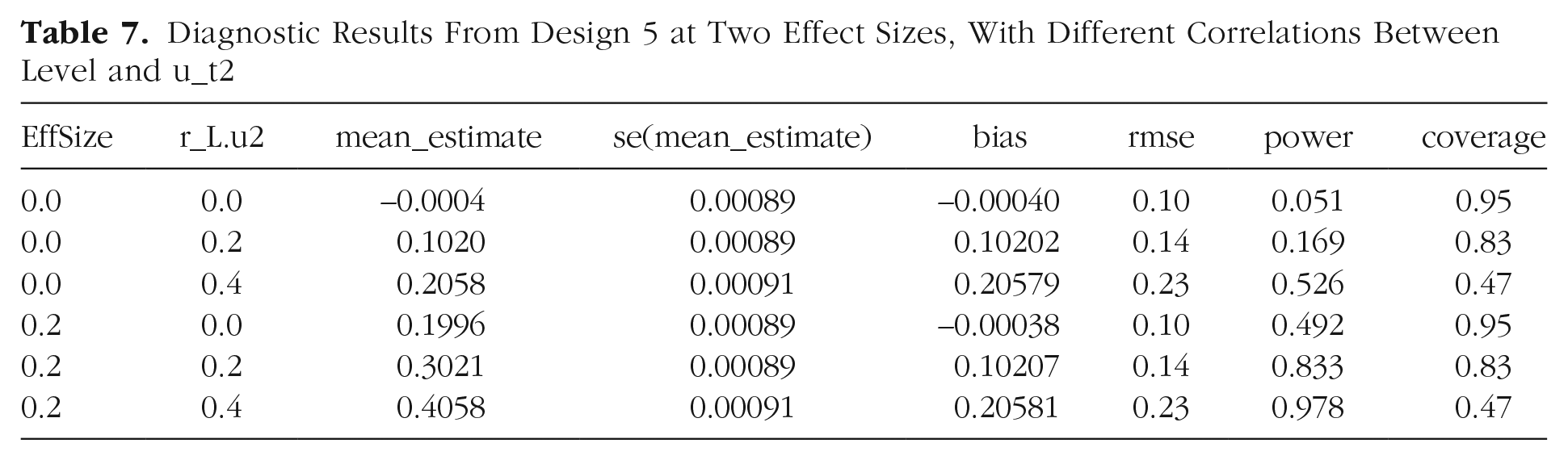
This simulation illustrates the importance of considering diagnosands that go beyond statistical power when evaluating designs. Design 4 gives high power estimates for the real effect of .2, but these are misleading because of the upward bias in estimates of intervention effect. When we look at the coverage statistic, which is the probability that the confidence interval around an estimate contains the true value, we see that the estimates from this design are very poor indicators of the true effect. In other words, a design that gives upwardly biased estimates of the intervention effect will have a low rate of false negatives (i.e., high power) but only because it has a high rate of false positives (see also Fig. 2). Discussions of research designs typically concentrate on power and whether an estimate is likely to be unbiased (as it is with a randomized experiment). These simulations demonstrate the importance of considering coverage as well as bias and power when discussing the effectiveness of a design. However, the simplest and most important message from Design 5 is that it quantifies the extent to which subverting the randomization process used in a trial can lead to substantial bias in estimating the causal effect of a treatment. In this case, selecting only those children who made progress as a result of an intervention and comparing them with the control group produces an artifactually inflated estimate of the effect of the intervention.

Distribution of estimates of effect size for original National Foundation for Educational Research design (Model 2) and Cambridge design (Model 6) when null hypothesis is true; 10,000 simulations. Dashed vertical line shows true effect size.
Design 6: Combining Designs 4 and 5
In a final set of simulations, we combined Designs 4 and 5 to create simulations that corresponded to the Cambridge reanalysis to consider the extent of bias introduced by the combination of multiple outcomes and participant selection. We focused just on the case in which the null hypothesis was true and specified that the correlation between the selection variable and outcome variables is .2. For each run of this simulation, we again used the “p.hack” function to select the outcome variable that gives the largest effect size (from the five outcomes that are considered). Figure 2 shows the estimates of effect size that are obtained when the correct value of effect size is zero for Design 2 (NFER analysis) and Design 6 (Cambridge reanalysis).
For the NFER analysis in which the randomization is respected and only one test is conducted, we obtain an unbiased estimate of the true effect (d = 0, Fig. 2, top). However, for the Cambridge analysis (see Fig. 2, bottom), it is clear that the combination of using multiple outcomes (Design 4) and discarding participants from the intervention group (Design 5) dramatically biases the estimates, giving a mean estimate of the effect size of 0.11 and a false-positive rate of 0.2 even though the amount of correlation between the selection variable and outcome is relatively modest (r = .2). The modeling with DeclareDesign helps clarify how two aspects of analysis that individually create some bias in estimates have a larger effect in combination.
Discussion
This tutorial illustrates how seemingly contradictory conclusions from different analyses of a data set can be understood by using simulations to diagnose the properties of different analytic strategies. We consider first the insights into analyses of RCTs, then the implications for evaluating GG, and finally, the potential of DeclareDesign more widely in psychology.
The analysis of RCTs
The contrast between Design 1 and Design 5 emphasizes the importance of using randomization to evaluate interventions. The simulations demonstrate clearly that analyzing subsets of data from an RCT can introduce bias into the estimates of the intervention effect because the randomization of allocating participants to conditions is broken. As demonstrated in Design 5, when randomization is broken and we select participants to include based on a variable (called here “level,” the level reached on GG), we introduce bias, or a systematic distortion of the true effect size. The degree of bias varies systematically with the extent to which level correlates with reading ability at Time 2. The higher that correlation, the more the estimated effect size is (artifactually) increased. When the correlation is zero, we obtain an unbiased (accurate) effect size. As the positive correlation gets larger, the estimated effect size gets (artifactually) larger. If level correlated negatively with the level of reading ability, we would obtain a negative effect, indicating artifactually that the intervention was harmful.
This general conclusion about the need to respect the original randomization in an RCT and not select subgroups post hoc has been known for decades in the literature on clinical trials but may not be appreciated outside that domain. This may be particularly the case when selection is less extreme than in the Cambridge reanalysis. A common form of post hoc subgroup analysis is referred to in clinical trials as per protocol analysis. This is an analysis that compares the control group with only those participants who completed the intervention. When some of the original participants are excluded, the remaining participants can no longer be considered as balanced as they were originally because of randomization. As discussed by Bishop and Thompson (2023), it may seem logical that one should exclude from analysis individuals who did not complete the intervention. However, dropouts are seldom random, and therefore, simply ignoring dropouts in an analysis is likely to introduce bias. The standard approach to avoid bias in such cases is to report intent-to-treat (ITT) analyses (i.e., to include data from all participants in the analysis of a trial whether or not they have complied and received the treatment). ITT analyses are possible, however, only if posttest data for participants who have dropped out can be collected. There is a large literature on how this case should be handled, which is beyond the scope of this article, but suffice it to say that reliance on people’s intuitions about appropriate analyses can be misleading (M. L. Bell et al., 2013).
In clinical trials, it has also long been recognized that outcomes should be preregistered and statistics adjusted if multiple tests are used. However, we suspect that this is another case in which researchers’ intuitions do not align with best practice. Many researchers do not understand how analyses may be seriously biased if these basic rules are broken. There may be good reasons for questioning the recommendation that a single primary outcome should be specified so that the problem of p-hacking is avoided. In the context of educational trials, it may be desirable to include a range of related outcome measures to maximize one’s chances of demonstrating an intervention effect when there is no obvious reason to prefer one measure over another. Bishop (2023) compared different approaches for handling this situation, noting that the popular method of applying a Bonferroni correction is overconservative when outcome measures are correlated. An alternative approach, “MEff,” is similar to Bonferroni correction but adjusts for intercorrelations between measures and is less conservative. However, in cases in which multiple measures are indicators of a common construct, the best way of avoiding the problems associated with doing independent analyses is to derive a latent construct that is defined by the variance that is shared between those measures (for an example in the field of language intervention, see West et al., 2021). Using a latent variable has the added advantage of increasing statistical power by eliminating error of measurement.
Once again, our main message is that with the simulations we have presented using DeclareDesign, we can quantify the consequences of deviating from recommended practice, including situations in which more than one bias is present, for example, when p-hacking is combined with bias from sample selection.
The effectiveness of GG Rime as a method of teaching reading
The RCT described here was designed to give a convincing answer to the question of whether GG Rime was an effective intervention for children who were struggling with learning to read. Although studies of GG had been conducted before this RCT, they were mostly small and quasi-experimental (McTigue et al., 2019). The effectiveness of GG Rime is a high-stakes issue given that according to the company’s website, it has been used by more than 4 million children and is an “effective, proven and affordable way to teach reading” and “the most researched literacy game in the world.” The contradictory claims arising from different analyses of the same study of the effectiveness of GG have led to confusion.
Our simulations show that having data from a large, well-powered RCT is not enough to guarantee secure conclusions: It is crucial that the appropriate analysis is conducted. The Cambridge reanalyses of the GG RCT used methods that introduced bias into estimates of intervention effects—selection of subgroups for analysis after the study is completed. The problems created by such approaches are well known in fields such as clinical trials and political science. For instance, in their guideline on the investigation of subgroups in confirmatory clinical trials, the Committee for Medicinal Products for Human Use (2019) stated, “From a formal statistical point of view, no further confirmatory conclusions are possible in a clinical trial where the primary null hypothesis cannot be rejected.” And in an article titled “How Conditioning on Posttreatment Variables Can Ruin Your Experiment and What to Do About It,” Montgomery et al. (2018) noted the dangers of practices such as “dropping participants who fail manipulation checks; controlling for variables measured after the treatment such as potential mediators; or subsetting samples based on post-treatment variables” (p. 760). All of these practices can lead to biased estimates. Unfortunately, the Cambridge reanalyses fall in this category; so contrary to the conclusions of Ahmed et al. (2020), we conclude that there is no convincing evidence that GG Rime is more effective than the business-as-usual control condition.
Potential of DeclareDesign for evaluating analytic designs in psychology
We argue that research in the “many analysts” tradition needs to move beyond documenting the variability of results from different analytic decisions and to use simulation to evaluate the consequences for different diagnosands. Simulation can be particularly useful when there is a clash between recognized best practice for analysis and researchers’ intuitions because it can illustrate how specific methods introduce biases that may not be obvious (Tintle et al., 2015). Simulation also provides a more principled approach to evaluating alternative analyses because it demonstrates how analytic choices affect results in a situation in which the truth is known—because we have specified it in our model. The DeclareDesign package allows researchers to set up models in which the null hypothesis is true or there is a genuine intervention effect and then consider how far different analytic choices affect the rate of false positives or false-negative conclusions or the accuracy or precision of the estimates of effect size. As noted by Blair et al. (2023), the optimal design may depend on which aspects of study outcomes one prioritizes: There may be a trade-off between the likelihood of false positives versus false negatives or between bias and precision of estimates. The key issue is that if researchers specify their model and analysis well enough to simulate it, they will be able to estimate these properties.
Note that in contrast to the bias seen in Designs 4, 5, and 6, the analytic approaches in Designs 2 (adjusting for clustering) and 3 (use of ANOVA rather than pretest covariate adjustment) had relatively little impact on results. This may help explain why researchers sometimes feel they can ignore advice from statisticians: It can seem as if they are encouraged to do a far more complex analysis, only to get the same result as for a simpler approach. Note that we cannot generalize from these simulations to all designs using clustering or covariate adjustment: There will be situations when these make an important difference. Our advice is that when different analytic options present themselves, simulated data can be invaluable in helping evaluate which is optimal—and which should be avoided.
We have focused on a type of research design, the RCT, for which there is already a great deal known about optimal methods of analysis, but DeclareDesign is extremely flexible and can be applied to a wide range of different types of experimental and observational designs used by psychologists. Blair et al. (2023) provided examples of applications to observational and experimental designs and to more complex designs involving behavioral games, structural estimation, and meta-analysis. In this regard, DeclareDesign is not just an R package but is better seen as a flexible tool kit that facilitates better research design by encouraging researchers to use simulation to clarify the model, inquiry, data strategy, and answer strategy implicit in their design.
Supplemental Material
sj-docx-1-amp-10.1177_25152459241267904 – Supplemental material for When Alternative Analyses of the Same Data Come to Different Conclusions: A Tutorial Using DeclareDesign With a Worked Real-World Example
Supplemental material, sj-docx-1-amp-10.1177_25152459241267904 for When Alternative Analyses of the Same Data Come to Different Conclusions: A Tutorial Using DeclareDesign With a Worked Real-World Example by Dorothy V. M. Bishop and Charles Hulme in Advances in Methods and Practices in Psychological Science
Footnotes
Acknowledgements
We are most grateful to Macartan Humphreys for clarification of technical issues relating to the DeclareDesign package. The R Markdown file “GGrmd.Rmd” creates the article and all analyses, including code that is not displayed in the article. The submitted draft was deposited as a preprint on PsyArxiv, https://osf.io/preprints/psyarxiv/vzg3e. The code to reproduce the analyses reported in this article is publicly available via the OSF and can be accessed at ![]() . This site also has the diagnosis files for 10,000 simulations of each of the six designs described in this article.
. This site also has the diagnosis files for 10,000 simulations of each of the six designs described in this article.
Transparency
Action Editor: David A. Sbarra
Editor: David A. Sbarra
Author Contributions
References
Supplementary Material
Please find the following supplemental material available below.
For Open Access articles published under a Creative Commons License, all supplemental material carries the same license as the article it is associated with.
For non-Open Access articles published, all supplemental material carries a non-exclusive license, and permission requests for re-use of supplemental material or any part of supplemental material shall be sent directly to the copyright owner as specified in the copyright notice associated with the article.