Sage Journals: Discover world-class research

Abstract

When new data are collected to check the findings of an original study, it can be challenging to evaluate replication results. The small-telescopes method is designed to assess not only whether the effect observed in the replication study is statistically significant but also whether this effect is large enough to have been detected in the original study. Unless both criteria are met, the replication either fails to support the original findings or the results are mixed. When implemented in the conventional manner, this small-telescopes method can be impractical or impossible to conduct, and doing so often requires parametric assumptions that may not be satisfied. We present an empirical approach that can be used for a variety of study designs and data-analytic techniques. The empirical approach to the small-telescopes method is intended to extend its reach as a tool for addressing the replication crisis by evaluating findings in psychological science and beyond. In the present tutorial, we demonstrate this approach using a Shiny app and R code and included an analysis of most studies (95%) replicated as part of the Open Science Collaboration’s Reproducibility Project in Psychology. In addition to its versatility, simulations demonstrate the accuracy and precision of the empirical approach to implementing small-telescopes analysis.

Keywords

small-telescopes analysis

One of the cornerstones of science is replicability. A single experiment does not hold the power to prove or disprove a particular theory. To be accepted by the scientific community, a theory must pass rigorous tests with consistent results. Despite the importance of reproducibility, many findings in psychology, as in other sciences, fail to replicate (Ioannidis, 2005; Maxwell et al., 2015; Shrout & Rodgers, 2018; Stroebe & Strack, 2014). Performing replication studies is worthwhile, but it also raises an important methodological question: How should replication results be evaluated? There are many recently developed methods to address this question, each with its own strengths and limitations (Maxwell et al., 2015; Nosek et al., 2022; Open Science Collaboration [OSC], 2015; Schauer & Hedges, 2021; Simonsohn, 2015; Stroebe & Strack, 2014).

Simonsohn (2015) proposed an approach known as the “small telescopes” method to more effectively evaluate replication results. This method involves performing a replication study with a larger sample than the original and assessing whether the newly measured effect is statistically significant and large enough to have been detectable using the original sample size. If both conditions are met, the original results are corroborated (Simonsohn, 2015). If not, the results either fail to support the original findings or are inconclusive. The small-telescopes method can be used to mitigate the replication crisis in psychology by directing the evaluation of results away from an exclusive reliance on tests of statistical significance. This method has gained traction in recent years; more than 750 citations were noted by Google Scholar as of August 2023. To help reach a more nuanced judgment, the small-telescopes method also draws on information provided by measures of effect size, confidence intervals (CIs), and statistical power to assess whether the original study was adequately powered to empirically support its conclusions.

Although the small-telescopes method is a promising tool for evaluating reproducibility, it does have some limitations. For instance, as described by Simonsohn (2015), using this method requires the calculation of an effect size, the construction of a CI for that effect size, and the estimation of statistical power for the lower and upper bounds of this CI. Simonsohn employed an analytic approach to these calculations, meaning that it requires formulas not only for calculating effect size but also for constructing CIs and estimating statistical power. This analytic approach does not necessarily involve complex math, and the required calculations may be performed using statistical software. For many common analyses, such as t tests and analyses of variance (ANOVAs), these formulas are widely available and relatively easy to use (Faul et al., 2007; Lee, 2016; Lenth, 2007). However, for other types of analyses, such as hierarchical regressions that control for covariates or assess interactions, multilevel models, focal effects obtained via structural equation models, or analyses of covariance, formulas to construct a CI and estimate power may not exist. Other times, one may wish to forgo formulas that require making parametric assumptions (e.g., normality, homogeneity of variance) that may be untenable for the data at hand. These distributional assumptions are mainly related to test statistics. Because of this, violations of assumptions can influence estimates of statistical power when a small-telescopes analysis is performed. When formulas are not available or one would rather not make parametric assumptions, one cannot implement the small-telescopes method as described by Simonsohn. To extend the reach of the small-telescopes method, we developed an empirical approach to its implementation that uses bootstrapping for CI construction and statistical power estimation. This versatile approach is available in a Shiny app and an R package, both of which are illustrated in the present tutorial. Finally, we used simulations to examine the accuracy and precision of the empirical approach to small-telescopes analysis.

Small-Telescopes Analysis

Background

To help explain this method, Simonsohn (2015) introduced an analogy. Suppose an astronomer observes a new planet with a telescope. To verify the existence of this planet, a second astronomer with a larger, more powerful telescope observes the same area of the sky. If the second astronomer can find the new planet, this corroborates its existence. On the other hand, if the second astronomer is unable to detect this new planet, this suggests that the original sighting may have been spurious. A planet observable using the small telescope should also be observable using the larger, more powerful telescope.

The key to using the small-telescopes method in psychological science is to begin with a replication sample size at least 2.5 times that of the original study, which is analogous to using a larger telescope in astronomy (Simonsohn, 2015). Next, the investigator addresses two questions. (a) Are the replication results statistically significant? (b) Given the effect size estimated in the replication study, would this have been detectable given the sample size of the original study? The four pairs of answers to these questions yield different conclusions.

Four possible conclusions

First, if the replication results are statistically significant and the original study appears to have been sufficiently powered, the original findings are supported. By analogy, this is when the use of a larger telescope both confirms the existence of a new planet identified using a smaller telescope and suggests that a planet of that size would have been detectable using the smaller telescope.

Second, if the replication results are not statistically significant and the original study appears to have been insufficiently powered, the original findings are not supported. By analogy, this is when the use of a larger telescope fails to confirm the existence of a new planet identified using a smaller telescope and also suggests that a planet of that size would not have been detectable using the smaller telescope.

In these first two possibilities, the evidence is consistent in reaching a conclusion. In the former case, the evidence supports the original findings. In the latter case, the evidence suggests that the original findings may have been spurious. However, this is not the only possible explanation. Other potential explications include a Type I error in the original study, a Type II error in the replication study, methodological differences between studies, and change in the studied phenomenon over time. The final two possibilities involve inconsistent evidence.

Third, if the replication results are statistically significant and the original study appears to have been insufficiently powered, the original findings are not supported. However, the replication results nonetheless provide some measure of support for the original conclusion. By analogy, this is when the use of a larger telescope does confirm the existence of a new planet identified using a smaller telescope but also suggests that a planet of that size would not have been detectable using the smaller telescope. The original claim may have rested on a questionable foundation, yet it may turn out to be correct nonetheless.

Fourth, if the replication results are not statistically significant and the original study appears to have been sufficiently powered, the evidence is inconclusive, and further research is needed to reach a more definitive conclusion. The telescope analogy breaks down in this instance. If the use of a larger telescope failed to detect a new planet, then presumably, it would not have been detectable using a smaller telescope. In psychological science, however, this pattern of results could emerge if the replication study did not follow Simonsohn’s (2015) advice of using a sample size 2.5 times larger than in the original study. This is analogous to doing small-telescopes analysis without having used a larger telescope.

Procedural overview

Addressing the question of whether replication results are statistically significant involves conventional tests that are not new to the small-telescopes method. What is new is the technique for addressing the question of whether the original study appears to have been sufficiently powered. This is the focus of our attention in how to perform a small-telescopes analysis.

The process begins with an estimate of the effect size in the replication study (Simonsohn, 2015). Given the use of a larger sample size, this is presumed to be a better estimate than one calculated from the original study results. Next, a CI is constructed around this effect size to account for sampling error in its estimation. Finally, statistical power at each end of the CI is estimated. This power is estimated using the sample size of the original research and the effect size (and its associated CI) in the replication study. The critical question is whether the CI of the replication study contains the smallest effect size that the original study would have sufficient power to detect. Simonsohn suggested using a 90% CI and operationalized sufficient power in this context as 33%. Therefore, if the 90% CI of the replication study contains the smallest effect size that the original study would have at least 33% power to detect, the original study is judged to be sufficiently powered. Otherwise, the original study is judged to be insufficiently powered.

An empirical approach

Simonsohn (2015) demonstrated how to implement the small-telescopes method analytically, constructing CIs and estimating power using available formulas. As noted earlier, for some types of data analysis, these formulas might not exist, or one might not be willing to make the required parametric assumptions. Our empirical approach implements the small-telescopes method in a four-step process that uses resampling techniques.

Step 1: test for statistical significance in replication data

This step is simple. Perform the appropriate test of statistical significance. This depends on the research design, but it should be the same type of test as in the original study.

Step 2: calculate effect size from replication data

This second step is also straightforward. Depending on the nature of the data and the type of statistical test, calculate an appropriate measure of effect size. This may or may not have been done in the original study, but if so, this can help to guide the choice of an appropriate measure.

Step 3: construct a 90% CI for the effect size

This is where the empirical approach first diverges from the analytic approach because resampling is used instead of formulas. Starting with the point estimate of effect size in the replication study, a CI is obtained through percentile bootstrapping (Efron & Tibshirani, 1993). This involves taking a large number of random samples (with replacement) from the data, calculating the effect size in each of those samples, and constructing the CI by choosing the effect sizes at the appropriate percentiles that form its lower and upper limits (Wood, 2004). For example, when constructing an interval with 90% confidence, as Simonsohn (2015) recommended for small-telescopes analysis, the lower bound of the interval will be the effect size at the fifth percentile, and the upper bound will be the effect size at the 95th percentile. In addition to enabling a CI to be constructed when no formulas are available to do so or when one simply prefers not to make their required assumptions, a bootstrapped CI cannot extend beyond the theoretically possible range of values. For example, whereas an analytic CI for a probability or a proportion of variance explained can extend below 0 or above 1, an empirical CI constructed via bootstrapping cannot.

Step 4: estimate statistical power for the lower and upper bounds of the CI

The empirical approach also uses resampling, rather than formulas, at this step of the process. Specifically, statistical power is estimated through bootstrapping. Bootstrapping is a widely used method of statistical power estimation (Efron & Tibshirani, 1993; Zhang, 2014), and we empirically evaluate its utility in the present context below. Using the bootstrap sample that yielded the effect size estimate at the fifth percentile (the lower bound of the CI), the researcher takes a series of random samples (with replacement), and power is estimated to be the proportion of times that a test of statistical significance rejects the null hypothesis in these samples. Once power has been estimated at the lower bound of the CI, the same thing is done to estimate power at the upper bound of the CI (using the bootstrap sample that yielded the effect size at the 95th percentile). Once again, this empirical approach enables one to proceed even when formulas for estimating statistical power are unavailable or one prefers not to make the required parametric assumptions.

The key to the small-telescopes analysis is that at this step in the process, statistical power is estimated using the sample size of the original study. This allows one to assess whether the original study would have been adequately powered to detect an effect whose size was estimated using the replication study, with its larger sample. This is what completes the analogy of using a larger telescope to evaluate the earlier findings obtained using a smaller telescope.

Step 5: interpret the results

As described earlier, evaluating replication results using small-telescopes analysis entails asking (a) whether the replication results are statistically significant and (b) whether the smallest effect size that the original study would have been adequately powered to detect is contained in the CI for the replication results. For example, suppose the effect of interest in the original and replication studies was a difference across three experimental conditions. Addressing the first question is done on the basis of the test of statistical significance performed in Step 1. In this example, one could use the F test from an ANOVA. Addressing the second question is done using the statistical power estimates from Step 4. In this example, it would entail estimating an appropriate measure of effect size, such as η²; constructing a 90% CI around this point estimate of effect size; and estimating statistical power at the lower and upper bounds of the CI. The original study is deemed sufficiently powered to detect the effect if the power estimate at the upper bound is at least 33% (a threshold suggested by Simonsohn, 2015). In the event that the effect of interest lies in the other direction (e.g., a negative correlation), one would examine the statistical power estimate at the lower bound, rather than the upper bound, of the 90% CI. Users need to estimate power at only one bound of the interval, but because the bound of interest depends on the research context, the present method provides power estimations for both bounds.

The five steps in this empirical approach to the small-telescopes method are displayed in Figure 1.

Fig. 1.

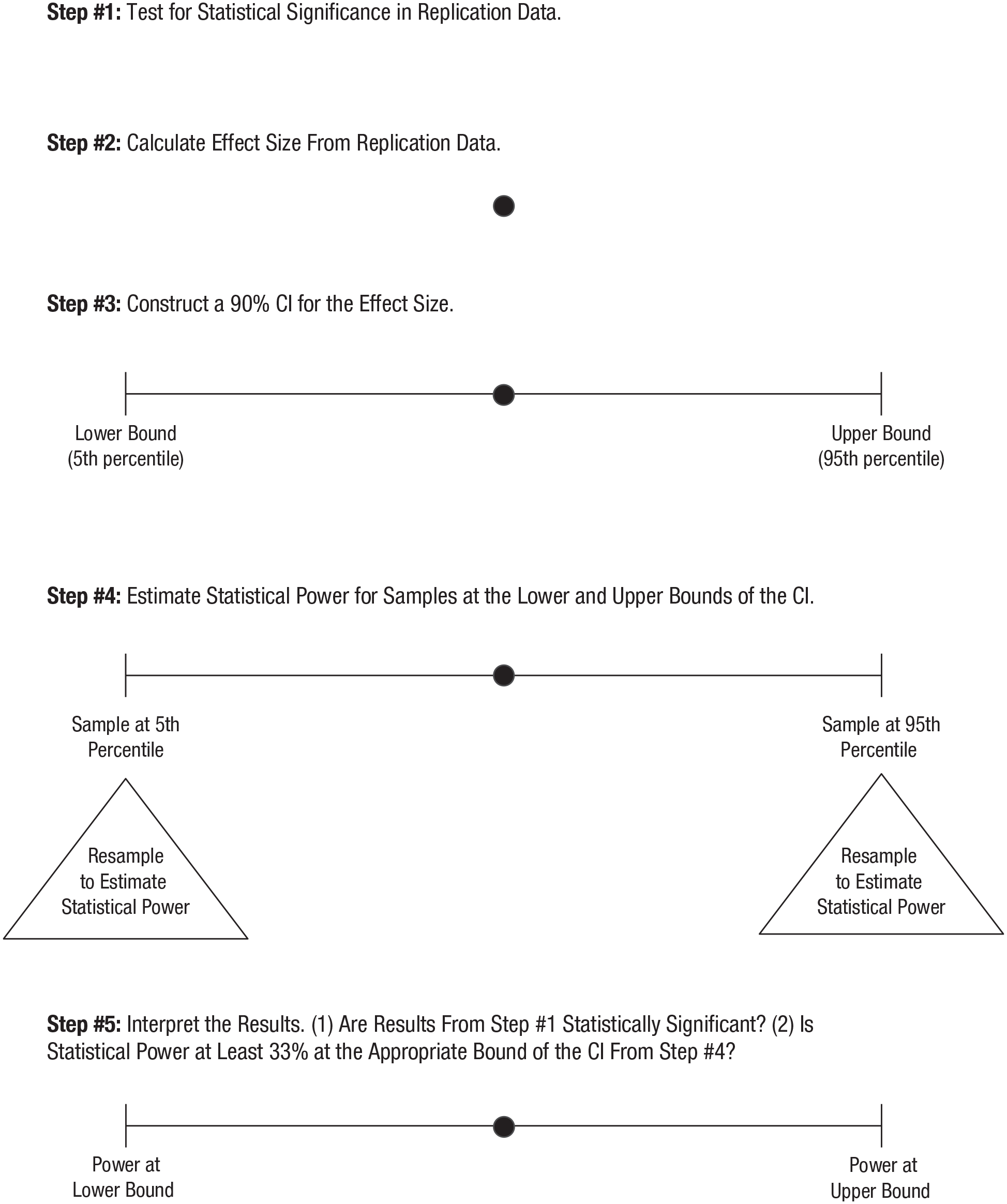
Steps in the empirical approach to small-telescopes analysis.

Tutorial

Shiny app

We begin with a demonstration of empirical small-telescopes analysis using the graphical user interface of the RSmallTelescopes Shiny app, and this is followed by showing how to use the RSmallTelescopes package in R. For both, we first work with a replication study conducted as part of the OSC’s (2015) Reproducibility Project in Psychology (RPP). Study 104, as numbered in the OSC archives, attempted to replicate an investigation of construal-level theory (Alter & Oppenheimer, 2008) that found that conceptually fluent objects were perceived more concretely and conceptually disfluent objects were perceived more abstractly, χ²(1, N = 236) = 3.83, p = .05, ϕ = .13. The replication study recruited approximately 5 times the original sample size, and when the key statistical test (a χ² test of independence with Yates’s continuity correction) was performed, the result was not statistically significant, χ²(1, N = 1,146) = 0.387, p = .543, ϕ = .018. More information regarding this study is available at https://osf.io/kegmc/.

To begin, access the RSmallTelescopes Shiny app at https://ruscio.shinyapps.io/RSmallTelescopes_app/. Once in the app, users will see a welcome message and widgets to input the information necessary to conduct the analysis. Figure 2 displays the app’s widgets. Users will need to upload the data as a comma-separated value (CSV) file in which each row contains the data for one subject and each column contains the data for one variable. Because the OSC archive for Study 104 provided the data in the form of a frequency table, we converted this to a CSV file in which there were 1,146 rows (one per subject) and two columns (one per variable). We confirmed that χ² analyses of the original frequency table and our CSV file yielded identical results. The CSV file used for this demonstration is titled “ao.csv” and is available at https://osf.io/4daw2/.

Fig. 2.

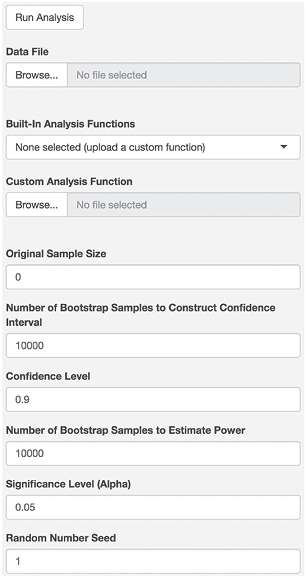
RSmallTelescopes Shiny app widgets.

After uploading their data, users have the option of choosing from five built-in functions to perform various simple analyses (correlation, independent-groups t test, related-samples t test, between-subjects ANOVA, and χ² test of independence) or uploading a custom analysis function. Choosing a built-in analysis is very straightforward, and for the present example, one could use the χ² test of independence function built into the Shiny app. Purely to demonstrate how one can go about creating a custom analysis function, we show how to do so here.

To obtain a p value and effect-size measure for this study design, one can use R’s chisq.test() function as shown below. In this case, the chisq.test() function returns the p value, and the effect size (a ϕ coefficient) can be calculated as the square root of the test statistic (χ², also provided by the chisq.test() function) divided by N (or the number of rows in the data). Our custom analysis() function returns a list object with two elements, effect.size and p.value:

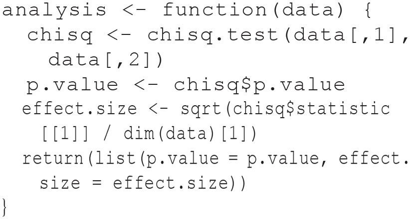
An R script containing this function is available at https://osf.io/4daw2/.

For any other type of analysis, the key to building a custom analysis() function to use in the Shiny app would be to return the same: a list object containing effect.size and p.value. Refer to Table 1 for a list of R functions and packages that one can draw from to calculate measures of effect size and obtain p values for many common types of data analysis.

Table 1.

List of R Packages and Functions to Calculate Effect Sizes and Obtain p Values

Analysis	R package	Function
Correlation	stats	cor.test
Regression	stats	lm
Multilevel model	lme4	lmer
Binomial test	stats	binom.test
Chi-square	stats	chisq.test
t test	stats	t.test
Analysis of variance	stats	aov
Levene’s test	car	leveneTest

Note: This illustrative list contains many of the types of analysis used in the Open Science Collaboration (2015) Reproducibility Project in Psychology (RPP). The stats package is available in the default R installation. Demonstrations of how to use all of these packages (and more) are available in the repository containing all code used to perform small-telescopes analyses for the RPP studies: https://osf.io/4daw2/.

In addition to uploading the data and perhaps a custom analysis file, users will specify a variety of parameters in the remaining widgets. This begins with the original sample size. Unlike each of the remaining widgets, there is no default value for the original sample size. For the present example, the original study had 236 subjects. As a default, a 90% CI will be constructed (following the recommendation of Simonsohn, 2015) using 10,000 bootstrap samples. Using 10,000 bootstrap samples is sufficient to produce stable estimates of the upper and lower bounds of a CI (Efron & Tibshirani, 1993) but not so large that it significantly slows analysis run time. For the present example, with replication study N = 1,146 and original study N = 236, the small-telescopes analysis ran in less than 1 min. The same was true when we tested each of the built-in analysis functions with test data. Unless one has a very large sample size or a computationally intensive type of data analysis, run time should not be a serious concern.

Statistical power is estimated for both ends of the CI despite the fact that the investigator will usually be interested in power at only one end, depending on the direction of the effect being investigated. When estimating power, a new layer of bootstrap samples is used, once again with a default of 10,000 samples. Given that the goal is to assess whether power exceeds 33% (following the advice of Simonsohn, 2015), estimation using 10,000 bootstrap samples should provide sufficient precision. As discussed later, we set default values conservatively to enhance precision; if run time is prohibitive for complex analyses of large data sets, the number of bootstrap samples used at one or both stages can be reduced.

Users can change the α level used for statistical significance when estimating power (default = .05). Finally, a random-number seed is set to make the analyses themselves reproducible. As a default, the seed is set to 1. Using the same random-number seed for a subsequent analysis of the same data would ensure that the bootstrap samples themselves would be the same rather than newly randomized. Alternatively, anyone curious about the impact that random sampling error in the bootstrapping process has on small-telescopes results could run the analysis multiple times, beginning with different random-number seeds, to check how consistent the results are. Using 10,000 bootstrap samples should provide good stability (Efron & Tibshirani, 1993), but if run-time considerations lead to reducing this, one can easily check on the stability of results by checking how much using other random-number seeds influences them.

Once the parameters of the app have been set, the analysis can be conducted by pressing the “Run Analysis” button. Notes shown in the app itself guide the user through the process and explain how a data file should be set up to use one of the built-in analysis functions. While the analysis is running, a progress bar will be displayed in the app. Figure 3 shows the output for the present example using the settings shown in Figure 2. The p value at the top of the output (p = .543) reveals that the replication results are not statistically significant. After constructing the 90% CI for the ϕ coefficient, statistical power is estimated at each bound using the original study’s sample size. The power estimate at the upper bound is only .150, which suggests that the original study was insufficiently powered. The largest effect that the original study would have had at least 33% power to detect is not contained within this 90% CI. Given this and the statistically nonsignificant replication results, the small-telescopes analysis fails to support the original findings.

Fig. 3.

Output from RSmallTelescopes app using Open Science Collaboration Study 104. Analysis was conducted on August 25, 2023.

Before proceeding, we note that it is encouraging that the statistical power estimate is similar to that obtained through an analytic implementation of the small-telescopes analysis for these data. Whereas the empirical approach yielded a power estimate of .150, the analytic approach (performed using the DescTools R package to construct the CI and the pwr package to estimate statistical power) yielded a power estimate of .181. The difference between these values—power estimates of 15.0% versus 18.1%—is inconsequential for decision-making because both are well below 33%. The difference of 3.1% is likely due to the fact that whereas the analytic approach makes assumptions regarding the shape of a hypothetical sampling distribution and, when estimating power, about its continuity (rather than discreteness in the analysis of nominal data), the empirical approach generates an observed sampling distribution through resampling and, when estimating power, works with only the discrete values observable in actual (bootstrap) samples of nominal data.

To demonstrate that the small difference in power estimates observed in this example are due to differences in assumptions regarding how to construct a CI and estimate statistical power and not problems with the code we wrote to implement the empirical approach to small-telescopes analysis, we performed a second analysis in which no differences in assumptions between the two approaches would be expected to lead to different results. The data representing the replication study were drawn from a bivariate normal distribution, with r = .135 in a sample of 1,000. The psychometric R package was used to construct an analytic 90% CI = [.083, .185], and the pwr R package was used to estimate power at both ends of the CI presuming the original study had N = 400: 90% CI = [.383, .962]. The empirical small-telescopes analysis yielded highly similar results: 90% CI = [.084, .184] and power estimates of (.384, .969). The bounds of the CIs and the power estimates all agreed within ±.01.

R package

In addition to using the RSmallTelescopes Shiny app, users have the option of conducting the analysis in R through the RSmallTelescopes package (available at https://cran.r-project.org/web/packages/RSmallTelescopes/index.html). The analysis is conducted in the same manner and with the same parameters, but the package offers added flexibility in terms of the format of a data file and the types of analyses that can be performed. Whereas the Shiny app requires a CSV file, users can upload data into R using a wide variety of formats (e.g., CSV, tab-delimited, SPSS, Excel). In addition, users can work with data for which each case spans more than a single row. More importantly, whereas the Shiny app has a relatively small number of commonly used types of data analysis built in, using the R package allows users to perform any type of analysis for which a p value and an effect-size measure are available. They can draw from an extensive library of other R packages or create their own code to perform analyses. Although this can be done through the Shiny app, too, by uploading a custom analysis() function in a text file, users comfortable creating such a file might find it simpler to do the entire small-telescopes analysis in R itself.

To begin, users will install the RSmallTelescopes package to access the SmallTelescopes() function. This conducts the empirical small-telescopes analysis, returning the p value from a test of statistical significance plus a CI and power estimate for the effect size measured in the replication study. To run the function, users specify the data to be used, the original sample size, the analysis function (which returns effect size and p value), and the optional parameters discussed above (e.g., number of bootstrap samples, confidence level, significance level). To demonstrate, here is how the same analysis shown earlier, for OSC Study 104, would be performed. First, install the package and upload the data:

Next, create an analysis function that returns an appropriate measure of effect size and a p value. The function for the present example has already been shown in the Shiny app section.

Finally, call the SmallTelescopes() function to perform the analysis. The arguments of the function correspond with the widgets of the app as shown in Table 2.

Table 2.

Shiny App Widgets and Corresponding R Package Function Arguments

Shiny app widgets	R package function arguments
Data File	data
Built-in Analysis Functions / Custom Analysis Function	analysis
Original Sample Size	n.original
Number of Bootstrap Samples to Construct Confidence Interval	B.CI
Confidence Level	CI.level
Number of Bootstrap Samples to Estimate Power	B.power
Significance Level (Alpha)	alpha
[not available in Shiny app]	n.rows
Random Number Seed	seed

For this example, the original sample size is 236, and the default settings will be used. The code below illustrates these parameters:

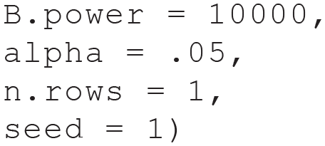
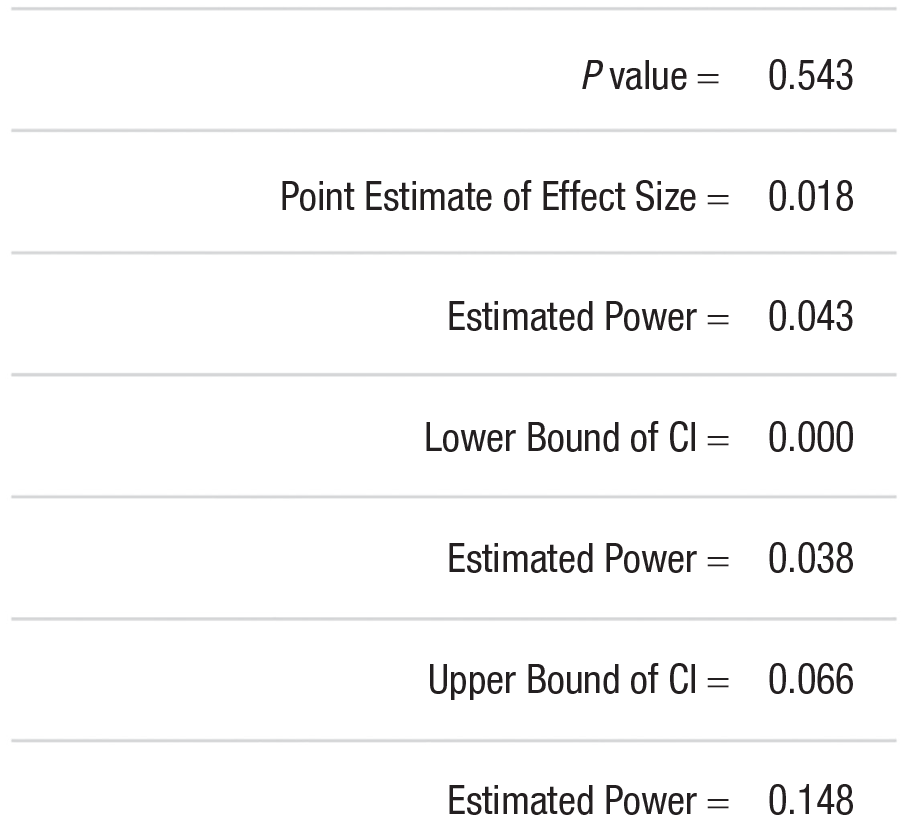
Figure 4¹ displays the output of the R package, which produces results nearly identical to those of the Shiny app. In particular, the p value was .543, and statistical power estimated at the upper bound of the CI was .148. The latter value differs slightly because of differences in random-number generation when using the Shiny app, hosted online, and the R package, running locally on a personal computer. As discussed earlier, one can examine how stable the results are by varying the random-number seed, which yields new bootstrap samples at each stage of the small-telescopes analysis. When the command shown above was rerun using seeds of 2 and 3, the power estimates at the upper bound of the CI were .149 and .147, which demonstrates strong agreement with the values of .150 from the Shiny app and .148 using the R package with seed = 1 (and leaves no doubt that the value falls short of the 33% threshold suggested by Simonsohn, 2015). Figure 5 summarizes the steps in the empirical small-telescopes analysis with results from this example. For this example, we can conclude that the original results are unsupported and that the original study was underpowered to detect the effect of interest. Although we cannot definitively conclude that the original results were a Type I error, it is not unreasonable to assume the replication results are more trustworthy given the significantly larger sample.

Fig. 4.

Output from SmallTelescopes() function using Open Science Collaboration Study 104. Analysis was conducted on August 25, 2023.

Fig. 5.

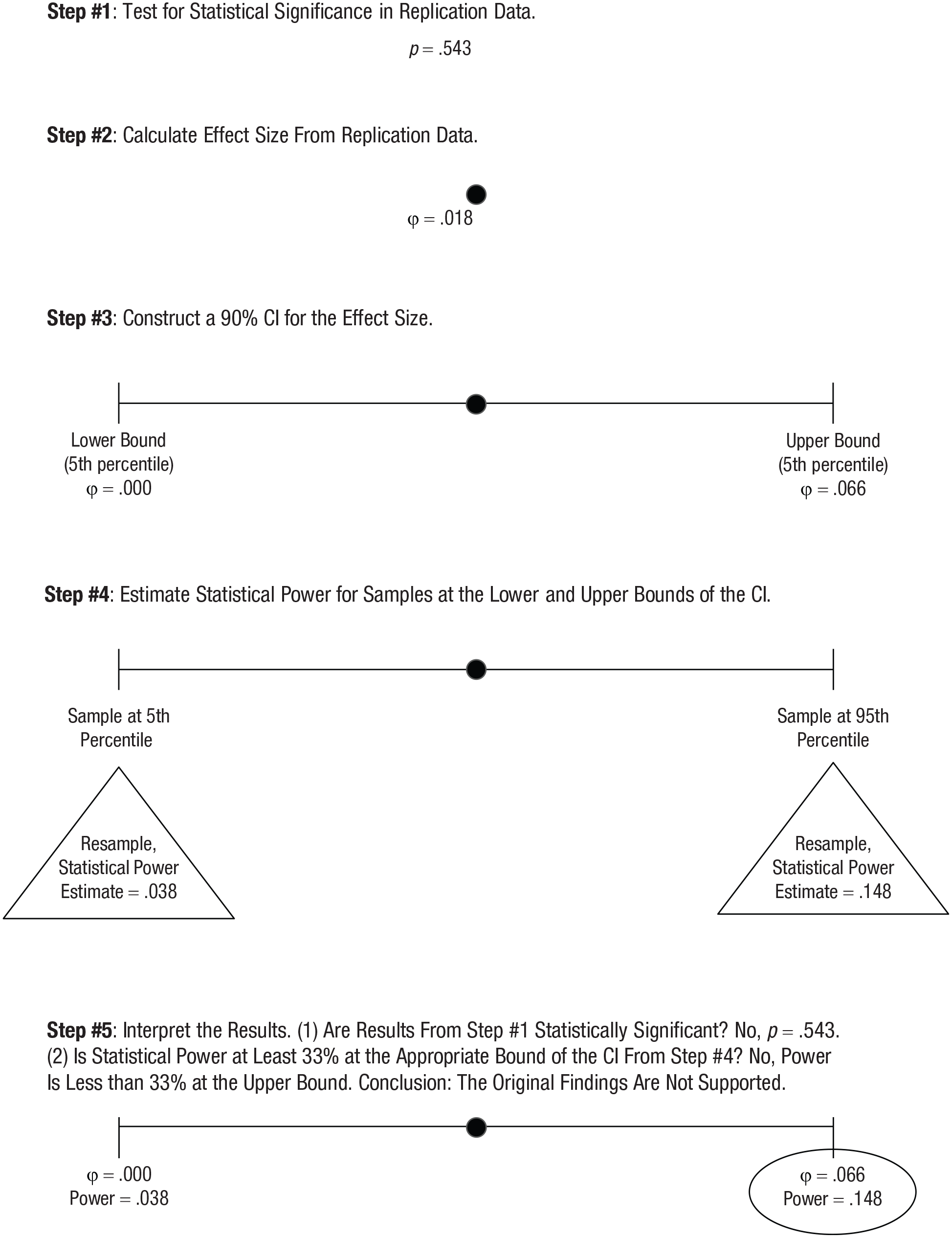
Steps in the empirical approach to small-telescopes analysis, illustrated with results from Open Science Collaboration Study 104.

Applications

The empirical approach to small-telescopes analysis has been used successfully in published research. For example, when evaluating the results of a series of replication studies, Crawford et al. (2019) were unable to take an analytic approach. In the original study, the investigators had conducted a regression analysis, and the effect of interest was an interaction tested after controlling for covariates and main effects. The replication authors were unable to identify formulas to estimate statistical power for the effect of interest in this scenario. By using an empirical approach, the authors were able to conduct the small-telescopes analysis.

To further demonstrate the utility and versatility of the empirical approach to small-telescopes analysis, we reanalyzed data from the OSC’s (2015) RPP. The RPP sought to evaluate the extent of false-positive findings in psychological science by replicating 100 studies chosen from leading social- and cognitive-psychology journals. The RPP was chosen for present purposes because it is well known and the data were readily available. All code used for this demonstration is available at https://osf.io/4daw2/.

The empirical small-telescopes analysis was conducted for 95 of the 100 studies. Studies 150 and 154, as numbered in the OSC archives, were excluded because we could not reproduce the results reported by the replication authors (and the OSC analysis auditors also failed to corroborate the reported results). Studies 25, 89, and 121 were excluded because the data management and analysis could not be conducted using an R package. In principle, however, the small-telescopes analysis could have been performed if these particular types of transposition error coding (Study 25), multilevel modeling (Study 89), and neuroimaging data-management techniques (Study 121) were available in R. Thus, before even considering the results, it is clear that the empirical approach to the small-telescopes method can be used for a wide range of study designs and analysis types. The limiting factor is not the availability of formulas for CI construction or statistical power estimation or the willingness to make parametric assumptions. Instead, the limiting factor is the availability of functions to perform the appropriate types of data analysis in R.

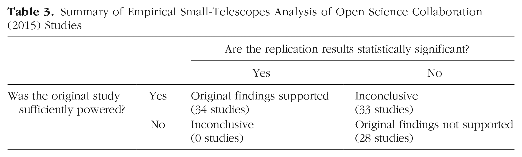
Thirty-four studies (36% of the 95 that were analyzed) supported the original results because the replication was statistically significant and the original study was sufficiently powered. Twenty-eight studies (29%), including the example shown above for OSC Study 104, did not support the original findings because the replication results were not statistically significant and the original study appeared to be underpowered. Thirty-three studies (34%) produced inconclusive results because the replication results were not statistically significant but the original study appeared to be sufficiently powered. This type of inconclusive results would not be expected to occur often, if ever, when designing a replication study with small-telescopes analysis in mind. However, the RPP was performed before Simonsohn (2015) published this method, and many of the RPP studies did not have a sample that was at least 2.5 times as large as the original. Finally, in no case were replication results statistically significant for an original study that appeared to be underpowered. Results are summarized in Table 3.

Table 3.

Summary of Empirical Small-Telescopes Analysis of Open Science Collaboration (2015) Studies

		Are the replication results statistically significant?
		Yes	No
Was the original study sufficiently powered?	Yes	Original findings supported (34 studies)	Inconclusive (33 studies)
	No	Inconclusive(0 studies)	Original findings not supported(28 studies)

Empirically Evaluating the Resampling Approach to Small-Telescopes Analysis

Simulations were performed to examine the accuracy and precision of the resampling approach to the small-telescopes method. Data were generated to simulate replication studies of two-group comparisons in which parametric assumptions of normality and equal variance were satisfied, which affords a comparison between the small-telescope results obtained via analytic calculations with those from resampling. The data conditions included equal group sizes in the original studies that were small (n = 25), medium (n = 50), or large (n = 100) and, as per Simonsohn’s (2015) advice, sample sizes were 2.5 times as large in the simulated replication studies. Effect sizes in these replication studies were sufficiently small (ds = 0.00, 0.05, or 0.10) that the independent-groups t tests were not statistically significant, and therefore a small-telescopes analysis would be warranted. The code used for this simulation is available at https://osf.io/4daw2/.

Within each cell of this 3 × 3 simulation design, standard analytic methods were used to implement small-telescopes analysis first by constructing a 90% CI for the effect size in the replication study and then by estimating statistical power at both ends of the CI using the sample size of the original study. These calculations provided reference values against which to compare the accuracy of results obtained via resampling. To assess its accuracy and the precision of its results, the resampling method was repeated 100 times for each data condition. The performance of the resampling method was tested not only using the default value of B = 10,000 bootstrap samples to construct CIs and to estimate statistical power but also smaller values of B = 1,000 and B = 100 to examine the impact of this parameter on the results.

Table 4 shows the analytically calculated CIs and statistical power estimates in bold. The results for resampling are summarized using the mean to assess accuracy and its standard error to assess precision. In the context of this resampling approach to small-telescopes analysis, one would expect greater precision when constructing CIs than when estimating statistical power. Constructing a CI entails a single application of the bootstrap, with its associated sampling error, whereas estimating statistical power relies on a second level of bootstrapping that introduces additional sampling error. Nonetheless, the simulation results reveal high levels of accuracy and precision at both stages.

Table 4.

Results for Simulated Replication Studies Testing the Mean Difference Between Two Groups

			Limits of 90% confidence interval for d		Statistical power estimates at limits of confidence interval
Original group size^a	Replication effect size and p value^b	Number of bootstrap samples^c	Lower bound	Upper bound	Lower bound	Upper bound
n = 25	d = 0.00	—	–0.294	0.294	0.179	0.179
	p = 1.000	10,000	–0.297 (0.004)	0.297 (0.003)	0.177 (0.008)	0.175 (0.009)
		1,000	–0.299 (0.012)	0.298 (0.013)	0.177 (0.018)	0.176 (0.019)
		100	–0.294 (0.043)	0.292 (0.034)	0.175 (0.050)	0.174 (0.042)
	d = 0.05	—	–0.245	0.344	0.137	0.229
	p = .780	10,000	–0.246 (0.004)	0.348 (0.004)	0.135 (0.007)	0.223 (0.010)
		1,000	–0.247 (0.012)	0.350 (0.013)	0.135 (0.014)	0.226 (0.020)
		100	–0.243 (0.044)	0.343 (0.035)	0.136 (0.046)	0.226 (0.048)
	d = 0.10	—	–0.195	0.394	0.102	0.286
	p = .576	10,000	–0.195 (0.004)	0.399 (0.004)	0.104 (0.006)	0.279 (0.009)
		1,000	–0.196 (0.012)	0.401 (0.013)	0.105 (0.013)	0.282 (0.021)
		100	–0.192 (0.044)	0.394 (0.036)	0.106 (0.040)	0.287 (0.053)
n = 50	d = 0.00	—	–0.208	0.208	0.179	0.179
	p = 1.000	10,000	–0.209 (0.003)	0.209 (0.002)	0.179 (0.006)	0.178 (0.006)
		1,000	–0.207 (0.008)	0.207 (0.007)	0.173 (0.016)	0.175 (0.016)
		100	–0.209 (0.027)	0.202 (0.023)	0.181 (0.057)	0.174 (0.043)
	d = 0.05	—	–0.158	0.258	0.121	0.252
	p = .693	10,000	–0.159 (0.003)	0.259 (0.002)	0.122 (0.004)	0.250 (0.007)
		1,000	–0.156 (0.008)	0.257 (0.007)	0.121 (0.013)	0.245 (0.019)
		100	–0.159 (0.027)	0.252 (0.024)	0.127 (0.046)	0.241 (0.059)
	d = 0.10	—	–0.109	0.308	0.078	0.337
	p = .429	10,000	–0.108 (0.003)	0.310 (0.002)	0.083 (0.004)	0.334 (0.007)
		1,000	–0.106 (0.008)	0.308 (0.007)	0.083 (0.010)	0.332 (0.020)
		100	–0.109 (0.028)	0.303 (0.024)	0.088 (0.035)	0.316 (0.057)
n = 100	d = 0.00	—	–0.147	0.147	0.179	0.179
	p = 1.000	10,000	–0.147 (0.002)	0.148 (0.002)	0.179 (0.005)	0.180 (0.006)
		1,000	–0.148 (0.007)	0.148 (0.006)	0.180 (0.016)	0.178 (0.015)
		100	–0.141 (0.017)	0.142 (0.016)	0.171 (0.048)	0.166 (0.051)
	d = 0.05	—	–0.097	0.197	0.102	0.286
	p = .576	10,000	–0.097 (0.002)	0.198 (0.002)	0.105 (0.004)	0.285 (0.008)
		1,000	–0.097 (0.007)	0.198 (0.006)	0.107 (0.012)	0.284 (0.020)
		100	–0.091 (0.016)	0.192 (0.016)	0.105 (0.035)	0.268 (0.063)
	d = 0.10	—	–0.047	0.247	0.062	0.416
	p = .264	10,000	–0.047 (0.002)	0.248 (0.002)	0.063 (0.003)	0.414 (0.008)
		1,000	–0.047 (0.007)	0.249 (0.006)	0.064 (0.009)	0.415 (0.023)
		100	–0.041 (0.016)	0.243 (0.016)	0.064 (0.025)	0.393 (0.070)

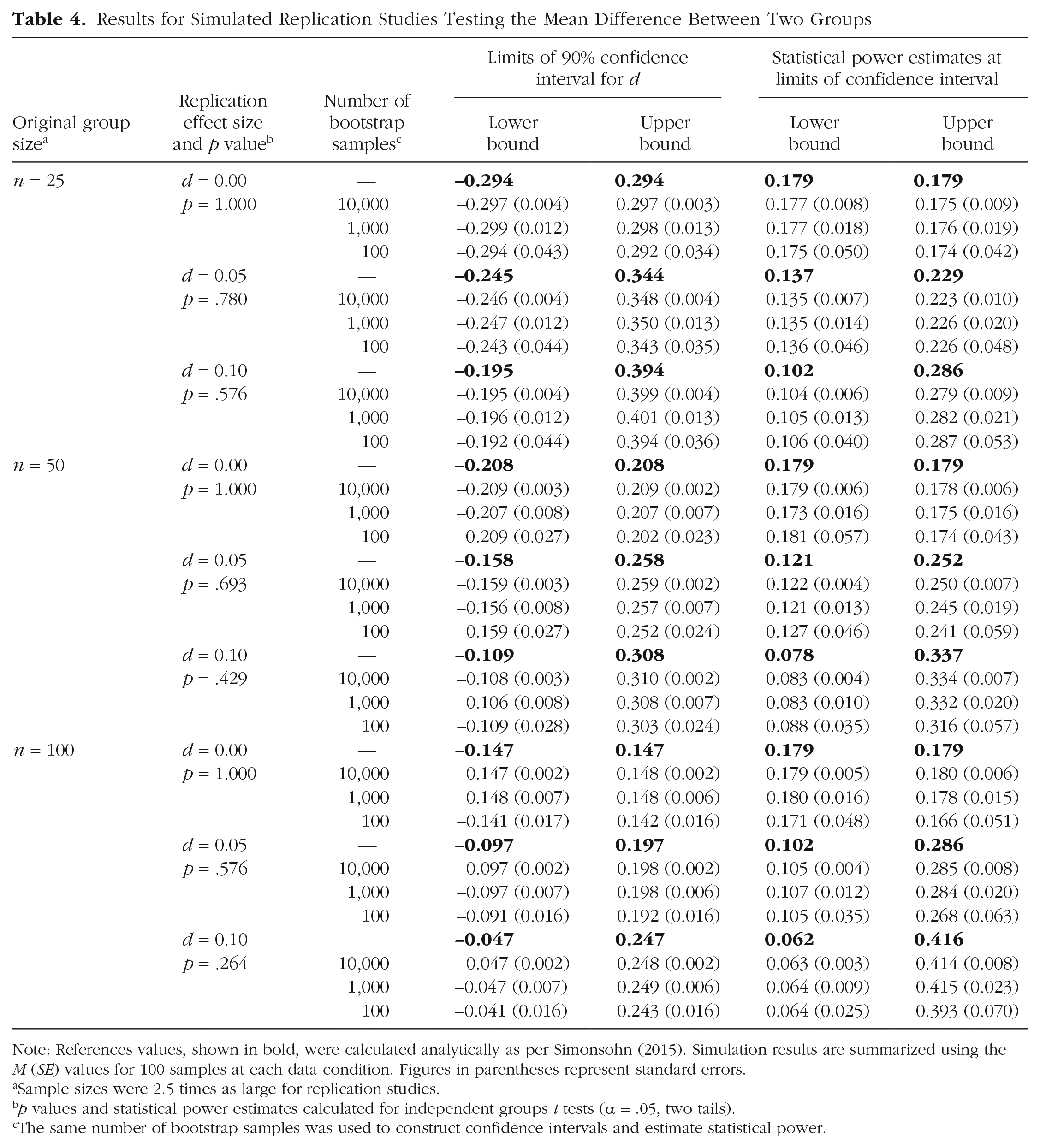
Note: References values, shown in bold, were calculated analytically as per Simonsohn (2015). Simulation results are summarized using the M (SE) values for 100 samples at each data condition. Figures in parentheses represent standard errors.

Sample sizes were 2.5 times as large for replication studies.

p values and statistical power estimates calculated for independent groups t tests (α = .05, two tails).

The same number of bootstrap samples was used to construct confidence intervals and estimate statistical power.

Using the program default of B = 10,000, most means were within ±0.001 of the calculated reference values, and none differed by more than ±0.007. Given the metrics of these CIs (Cohen’s d) and statistical power (probability scale), this represents excellent accuracy. Moreover, standard errors ranged from 0.002 to 0.010, which represents excellent precision. As expected, precision was even better for CIs (all SEs ≤ 0.004) than for statistical power estimates, but all of these values are quite small. This suggests that the resampling approach to small-telescopes analysis can be relied on to produce trustworthy results.

Finally, the influence of using fewer bootstrap samples to construct CIs and estimate statistical power was examined. Accuracy levels remained fairly high (most means remained within ±0.010 of reference values, and the largest difference was 0.023), but precision decreased (standard errors ranged as high as 0.023 for B = 1,000 and 0.070 for B = 100). This suggests that it would be wise to use the program default values of B = 10,000 bootstrap samples for CI construction and statistical power estimation unless run time is prohibitive. As a point of reference, an ordinary laptop computer took about 16 s to complete the small-telescopes analysis of each simulated replication study reported here when using B = 10,000.

Summary

The small-telescopes method proposed by Simonsohn (2015) provides a compelling way to evaluate replication results. However, performing small-telescopes analysis using an analytic approach is not always possible (if the required formulas do not exist), practical (if formulas exist but the calculations are not implemented in accessible software), or advisable (if parametric assumptions are violated), which limits how widely the method can be adopted. The empirical approach to small-telescopes analysis is a versatile tool for evaluating replication results because it can be used with a wide range of data analyses and data conditions. This approach allows users to conduct small-telescopes analysis even when the analytic approach is impractical or impossible to conduct, avoids making assumptions that may not be satisfied, yields only theoretically possible CI limits, and can be performed using freely available software.

The small-telescopes method can be used for a variety of study designs, and its particular strength is that its conclusions are based on more nuanced considerations than a test of statistical significance alone (Schauer & Hedges, 2021). By also asking whether the original study appears to have been adequately powered, one can reach a better-informed conclusion regarding the findings (Nosek et al., 2022).

In some instances, the original findings will be supported by a statistically significant replication and a small-telescopes analysis that suggests the original study was sufficiently powered to detect the effect. In other instances, the original findings will not be supported, as when the replication findings are not statistically significant and a small-telescopes analysis suggests the original study was insufficiently powered to detect the effect. Other patterns of results might suggest that the original findings were correct, albeit by a lucky accident, or that the findings of the original and replication studies are inconsistent, requiring further research to help reach a more definitive conclusion.

The ability to perform small-telescopes analysis empirically extends its reach, but there are also some limitations to this approach and what is known about it. One practical limitation is that it requires investigators to go beyond a test of statistical significance. Whether one wishes to perform small-telescopes analysis analytically or empirically, there is extra effort involved. The analytic approach requires identifying and using relevant formulas. Some or all of this may be facilitated by software, but that requires access to the software and knowing how to use it correctly. The empirical approach would be fairly simple if one’s analysis is of a common variety included in the Shiny app, less so if one’s analysis required the use of the R package. Although not a trivial concern, R is becoming increasingly familiar to psychological scientists, especially to younger investigators more likely to have been trained in it during graduate school, so this should not be too serious an obstacle to overcome if performing a small-telescopes analysis seems worthwhile.

In addition, although the empirical approach expands the usability of small-telescopes analysis, it is not necessarily well suited for all data and research designs. For instance, data with complex dependencies, such as nested or time-series data, cannot be analyzed with the present code. To conduct small-telescopes analysis in such cases, the code must be altered to use specialized bootstrap methods that ensure the resampling occurs at the proper unit of analysis.

Furthermore, whereas the analytic approach will usually require parametric assumptions, the empirical approach avoids these by resampling using bootstrap methods. However, this substitutes a different assumption: that the sample of data at hand is representative of its population (Efron & Tibshirani, 1993). For example, when one performs a t test to compare scores across two groups, one makes parametric assumptions about normality and homogeneity of variance. Using the bootstrap avoids those assumptions, instead assuming that the observed distributional shapes and variances are representative of individuals in the population. This may be more tenable than standard parametric assumptions in many instances, but particularly with small samples, there is no assurance that characteristics of the sample are representative of the population.

In addition to the different types of assumptions that the empirical approach makes, there are some additional uncertainties introduced by its implementation. Perhaps most significant is that we have not systematically studied the impact of varying the number of bootstrap samples that are used when constructing a CI and then when estimating statistical power at each end. We relied heavily on the advice of Efron and Tibshirani (1993), experts in bootstrap methods, and set default values even more conservatively than recommended to yield stable estimates. Particularly given that this is a two-stage process, using bootstrapping (for statistical power estimation) layered within bootstrapping (for the construction of a CI), we chose to err on what we believe is the side of caution by setting default values larger than is likely to be necessary to obtain sufficiently precise results for making decisions.

Future research could investigate the performance of this methodology using varying numbers of bootstrap samples at each stage. This could be done for a variety of types of data analysis because it is conceivable that smaller numbers of bootstrap samples are required to obtain sufficiently precise results for some types of analyses than for others. Until this issue is itself addressed empirically, we expect that leaving the number of bootstrap samples at the very large default values (10,000 samples at each stage) should be a safe way to proceed. If doing so takes too long to run a small-telescopes analysis, one can reduce the number of bootstrap samples at one or both stages. In that case, we recommend repeating the entire small-telescopes analysis using at least a few different random-number seeds to check whether the results are sufficiently stable to afford trustworthy conclusions.

Another area that might be worth exploring further is the bootstrap method used to construct a CI. We used the percentile bootstrap for several reasons. First, it is simple to understand and implement. Second, it generally works well, yielding CIs with good probability coverage (Efron & Tibshirani, 1993). Third, and perhaps most important, it enabled us to identify the precise bootstrap samples that yielded particular effect sizes. For example, when constructing a 90% CI, we wanted to know precisely which samples yielded effect sizes at the fifth and 95th percentiles. This is important because it allowed us to take these bootstrap samples and, in turn, perform the second-stage bootstrap resampling to estimate statistical power at each end of the CI. It is possible that another method of bootstrap CI construction would work even better, but that alternative would have to identify a unique bootstrap sample corresponding to each end of the CI. Interested readers can find further discussion of alternative bootstrap methods and software implementations in Banjanovic and Osborne (2016) and Kirby and Gerlanc (2013).

One interesting candidate that we considered is the bias-corrected and accelerated bootstrap method (Efron & Tibshirani, 1993). This often yields even better coverage probabilities than the percentile bootstrap method, and it would identify which samples yielded effect sizes at each end of a CI, but we have not yet included it in our small-telescopes software because it is more computing-intensive. Future research could examine whether the bias-corrected and accelerated bootstrap method produces results that are worth the increase in run time. For the time being, we believe the percentile bootstrap rests on a sufficiently solid theoretical foundation that it provides a good general-purpose CI construction method for the many types of data analyses encountered in replication studies.

With these limitations and unknowns in mind, we believe that the empirical approach to the small-telescopes method, as demonstrated through this tutorial, should enable this valuable tool to be used more often as researchers grapple with the replication crisis in psychological science and beyond.

Footnotes

Transparency

Action Editor: David A. Sbarra

Editor: David A. Sbarra

Author Contributions

Samantha Costigan: Conceptualization; Data curation; Formal analysis; Methodology; Software; Writing – original draft.

John Ruscio: Conceptualization; Investigation; Methodology; Project administration; Resources; Software; Supervision; Validation; Writing – review & editing.

Jarret T. Crawford: Conceptualization; Supervision; Validation; Writing – review & editing.

ORCID iDs

Samantha Costigan

Jarret T. Crawford

Notes

References

Alter

A. A.

Oppenheimer

D. M.

(2008). Effects of fluency on psychological distance and mental construal (or why New York is a large city, but New York is a civilized jungle). Psychological Science, 19, 161–167. https://doi.org/10.1111/j.1467-9280.2008.02062.x

Banjanovic

E. S.

Osborne

J. W.

(2016). Confidence intervals for effect sizes: Applying bootstrap resampling. Practical Assessment, Research, and Evaluation, 21, Article 5. https://doi.org/10.7275/dz3r-8n08

Crawford

J. T.

Fournier

Ruscio

(2019). Does subjective SES moderate the effect of money priming on socioeconomic system support? A replication of Schuler and Wänke (2016). Social Psychological and Personality Science, 10(1), 103–109. https://doi.org/10.1177/1948550617740941

Efron

Tibshirani

(1993). An introduction to the bootstrap. Chapman & Hall.

Faul

Erdfelder

Lang

A. G.

Buchner

(2007). G*Power 3: A flexible statistical power analysis program for the social, behavioral, and biomedical science. Behavior Research Methods, 39(2), 175–191. https://doi.org/10.3758/BF03193146

Ioannidis

J. P. A.

(2005). Why most published research findings are false. PLOS Medicine, 2, Article e124. https://doi.org/10.1371/journal.pmed.0020124

Kirby

K. N.

Gerlanc

(2013). BootES: An R package for bootstrap confidence intervals on effect sizes. Behavior Research Methods, 45, 905–927. https://doi.org/10.3758/s13428-013-0330-5

Lee

D. K.

(2016). Alternatives to P value: Confidence interval and effect size. Korean Journal of Anesthesiology, 69(6), 555–562. https://doi.org/10.4097/kjae.2016.69.6.555

Lenth

R. V.

(2007). Statistical power calculations. Journal of Animal Science, 85(13), 24–29. https://doi.org/10.2527/jas.2006-449

10.

Maxwell

S. E.

Lau

M. Y.

Howard

G. S.

(2015). Is psychology suffering from a replication crisis? What does “failure to replicate” really mean? American Psychologist, 70(6), 487–498. https://doi.org/10.1037/a0039400

11.

Nosek

B. A.

Hardwicke

T. E.

Moshontz

Allard

Corker

K. S.

Dreber

Fidler

Hilgard

Kline Struhl

Nuijten

M. B.

Rohrer

J. M.

Romero

Scheel

A. M.

Scherer

L. D.

Schönbrodt

F. D.

Vazire

(2022). Replicability, robustness, and reproducibility in psychological science. Annual Review of Psychology, 73, 719–748. https://doi.org/10.1146/annurev-psych-020821-114157

12.

Open Science Collaboration. (2015). Estimating the reproducibility of psychological science. Science, 343(6251), Article aac4716. https://doi.org/10.1126/science.aac4716

13.

Schauer

J. M.

Hedges

L. V.

(2021). Reconsidering statistical methods for assessing replication. Psychological Methods, 26(1), 127–139. https://doi.org/10.1037/met0000302

14.

Shrout

P. E.

Rodgers

J. L.

(2018). Psychology, science, and knowledge construction: Broadening perspectives from the replication crisis. Annual Review of Psychology, 69, 487–510. https://doi.org/10.1146/annurev-psych-122216-011845

15.

Simonsohn

(2015). Small telescopes: Detectability and the evaluation of replication results. Psychological Science, 26(5), 559–569. https://doi.org/10.1177/0956797614567341

16.

Stroebe

Strack

(2014). The alleged crisis and the illusion of exact replication. Perspectives on Psychological Science, 9(1), 59–71. https://doi.org/10.1177/1745691613514450

17.

Wood

(2004). Statistical inference using bootstrap confidence intervals. Significance, 1(4), 180–182. https://doi.org/10.1111/j.1740-9713.2004.00067.x

18.

Zhang

(2014). Monte Carlo based statistical power analysis for mediation models: Methods and software. Behavior Research Methods, 46(4), 1184–1198.