Sage Journals: Discover world-class research

Abstract

Topic modeling is a type of text analysis that identifies clusters of co-occurring words, or latent topics. A challenging step of topic modeling is determining the number of topics to extract. This tutorial describes tools researchers can use to identify the number and labels of topics in topic modeling. First, we outline the procedure for narrowing down a large range of models to a select number of candidate models. This procedure involves comparing the large set on fit metrics, including exclusivity, residuals, variational lower bound, and semantic coherence. Next, we describe the comparison of a small number of models using project goals as a guide and information about topic representative and solution congruence. Finally, we describe tools for labeling topics, including frequent and exclusive words, key examples, and correlations among topics.

Keywords

child development health infant natural language processing structural topic modeling topic modeling

Topic modeling is a type of text analysis that identifies clusters of co-occurring words, or latent topics (Jackson et al., 2022; Wallach, 2006). Topics provide one way to map the semantic structure of a set of documents, referred to as the “corpus.” For the psychological scientist, topic modeling can provide great utility describing the broad themes of a corpus (set of texts) and quantifying the degree to which a theme is present in a specific text. Researchers who collect text-based data (e.g., narratives, interviews, writing primes, and even survey questions) may find that topic modeling supplements or, in some cases, replaces human coding, thus saving resources (Jackson et al., 2022). Moreover, the ability for topic modeling to scale to thousands of documents facilitates its use in large data sets (Banks et al., 2018). For example, topic modeling has been used to study open-ended survey questions (Finch et al., 2018) and tweets in specific communities (Bedford-Petersen & Weston, 2021). Note that topic modeling is a good tool for uncovering broad subject-matter-based themes but not subtle nuances, which will still require human coding.

Several different algorithms are available for topic modeling (Blei et al., 2003; Fu et al., 2021; Valdez et al., 2018). Perhaps one of the simplest algorithms is latent Dirchlet allocation (LDA; Blei et al., 2003), which intuits that each document is a mixture of multiple topics (for an intuitive summary of probabilistic topic modeling, see Blei, 2012). Variations on LDA typically relax core assumptions in an effort to better represent a corpus or answer specific research questions. We have summarized several variations on topic modeling in Table 1. For individuals who are new to topic modeling, we recommend tutorials by Maier et al. (2018), Banks et al. (2018), and Schmiedel et al. (2019).

Table 1.

Examples of Variations on Topic Modeling

Name	Description
Latent Dirchlet allocation (Blei et al., 2003)	A simple algorithm that assumes a three-level hierarchical Bayesian model. Documents are modeled as random and finite mixtures of topics. Assumes words in a document are unordered.
Dynamic topic models (Blei & Lafferty, 2006)	Incorporates probabilistic time series to analyze the evolution of topics over time.
Correlated topic models (Blei & Lafferty, 2007)	Explicitly models the covariation among topics. See also Pachinko allocation (Li & McCallum, 2006), which estimates correlations between pairs of topics.
Structural topic models (Roberts et al., 2014)	Allows for the inclusion of metadata to analyze topic prevalence and content as a function of covariates.

A challenging step of topic modeling is determining the number of topics to extract. In this tutorial, we describe tools researchers can use to identify the number and labels of topics in topic modeling. There is likely no single correct number of topics for any corpus but, rather, several good options, each of which may be useful. Thus, topic modeling requires subjective decision-making informed by the data and research questions. In the case of open-ended survey questions, one might consider the specificity of the prompt, the total number of responses, and the relative length of those responses. A final consideration is practical: Solutions with more topics take more time and computer memory to evaluate and are difficult to label.

In the current tutorial, we aim to provide guidance for (a) identifying the number of topics to estimate while using topic modeling and (b) labeling those topics. This is in contrast to existing topic-modeling tutorials, which tend to cover a wide range of considerations (algorithm select, preprocessing, number of topics, and covariates) in less detail; here, we provide deep focus on one aspect of topic modeling. We assume that readers are familiar with topic modeling and the basic steps of conducting topic-modeling analysis. Although we demonstrate some of the essential steps in topic modeling (e.g., data cleaning), we do not discuss these in detail. We refer readers to work by others (Banks et al., 2018; Schmiedel et al., 2019) who have covered such aspects of topic modeling. The tutorial here is applicable across most topic-modeling algorithms; we chose to use structural topic modeling (STM) here as our example. This algorithm may be of special interest to psychologists because of its ability to include prevalence and content covariates (Roberts et al., 2014). In addition, its use of deterministic initialization limits concerns of topic reliability (Maier et al., 2018; Rieger et al., 2020).

Tutorial

Software

All analyses are conducted in R (Version 4.1.3; R Core Team, 2022). This tutorial primarily demonstrates functions available in the stm (Roberts et al., 2019) and tidytext (Silge & Robinson, 2016) packages, although we also use the suite of tidyverse (Wickham et al., 2019) packages for data cleaning and visualization. The stm package conducts topic modeling using the STM algorithm, and the package is well suited for use in R. However, the basic principles described in this tutorial apply to a wide variety of topic models.

Data description

Data come from the Rapid Assessment of Pandemic Impact on Development–Early Childhood project, a nationally representative sample of parents ages 5 and younger (approved by the University of Oregon Institutional Review Board, No. 03252020.031). All surveys included a set of variables assessing parent and child functioning. Special topics were included periodically, including the focus of this tutorial: an open-ended question, “How do you feel about the COVID-19 vaccine in terms of its safety and effectiveness, and what are your plans in terms of whether or not to get it?” This question was administered biweekly between March and December 2021 to 3,331 parents. Participants provided data an average of 1.96 times (maximum = 9), for a total of 6,516 observations. Data and code are available for download at https://osf.io/4nt8x.

These data represent a situation common to psychology researchers collecting longitudinal data: Responses to open-ended questions contain useful information about the population under study. Note that the researcher may not have developed survey questions to probe this information. In the case of these data, it was not known what types of issues would be relevant to child vaccination at the time of writing survey questions. However, a challenge to using the data is their unstructured nature. Topic modeling can provide such structure and also facilitate rapid assessment of thousands of responses.

Data cleaning

To prepare for text analyses, we chose to omit numbers, special characters, common stop words (e.g., prepositions and articles; for more information, see help page for the textProcessor() function), and words with fewer than 20 uses.¹ In some cases, stemming may also be appropriate at this stage (Valdez et al., 2018). Stemming reduces the number of terms by converting different words to the same root, for example, by converting both “writing” and “writer” to the stem “writ-”. However, recent work suggests that stemming does not produce meaningful improvement in model fits and can degrade stability (Schofield & Mimno, 2016). Thus, we did not stem words. Very common terms may also be removed, bespoke lists of stop words can be constructed, and bigrams and trigrams—two-word and three-word sets (e.g., “psychological science”)—can be concatenated before analysis. Basic preprocessing can be performed using the function textProcessor() from the stm package (see Fig. 1).

Fig. 1.

Preparing the text for topic modeling.

The documents argument refers to the open-ended responses collected from our survey (i.e., the variable labeled “vaccine”). Metadata is all other data you wish to be associated with responses, such as time and participant characteristics. Next, remove words with especially low frequencies. The function plotRemoved() may be useful for assessing the threshold at which to include words. A consequence of this step is that some responses are rendered empty, having also removed stop words. Not only do these responses need to be removed, but also all corresponding metadata requires removal to ensure that metadata are appropriately linked to each response. The prepDocuments() function handles both steps.

Narrowing down candidate models

How many and which?

The general procedure for identifying the ideal number of topics is to (1) examine the fit statistics of numerous possible solutions, (2) narrow down these solutions to a tractable number of candidate models, and (3) select one (or a small number) of models for further evaluation. Corpora can contain as few as three and as many as hundreds of topics. This is related both to the researcher’s goals and the number, length, and complexity of responses in the corpora. For instance, researchers have used as many as 65 (Jeong et al., 2019) and as few as eight (Edelmann et al., 2017) topics. In identifying the maximum number of possible topics, researchers should consider the number and length of responses and the specificity of the prompt. These should be intuitive: More (and longer) responses create opportunities for more topics, and specific questions restrict such opportunities. In the case of our example data, we have a relatively large number of responses, but the prompt is specific. Given the latter, we anticipated a relatively small number of dominant themes. Therefore, we extracted an upper bound of 20 topics.

Researchers choose the range and sequence of solutions to examine in the first round. If one is uncertain about the number of topics in a large corpus, one might look at solutions between five and 100 by five in the first round and then narrow the range and sequence in a subsequent round. Given our low maximum, we chose to extract all possible solutions up to 20 topics: from three (the minimum allowed) up to 20. When choosing specific values within a range to estimate, note the diminishing returns: That is, the gain in information from five to six topics is large, whereas the gain from 75 to 76 is small.

Statistics for comparisons

Once the initial set of possible solutions is identified, one can use the searchK() function in the stm package to efficiently² estimate all solutions and extract fit statistics for comparison (see Fig. 2). We note several relevant arguments: K is the set of solutions to be evaluated, such as three through 20, but this can be any vector of integers representing solutions of interest. The argument N indicates the number of documents to be held out from initial estimation. These held-out documents form a test sample with which candidate solutions are evaluated. Specifically, the searchK() function will estimate the likelihood fit values for these held-out documents. However, this may also affect estimates of other metrics discussed here (Maier et al., 2020). For small corpora, researchers may wish to use the entire set of documents. The argument init.type is used to set the method of initialization. There are several options available for this argument, but Spectral is expected to perform well in many cases (Roberts et al., 2019). Finally, heldout.seed takes any integer and ensures reproducibility.

Fig. 2.

Comparing candidate topic-model solutions on a series of fit statistics. exclus = exclusivity, lbound = variational lower bound, semcoh = semantic coherence.

Upon completion, the output object—which we called “storage”—contains for each candidate solution the values of several fit statistics. We recommend plotting these values for comparison (see Fig. 2). Exclusivity represents the degree to which words are exclusive to a single topic rather than associated with multiple topics. Exclusive words are more likely to carry topic-relevant content, thus assisting with the interpretation of topics (Airoldi & Bischof, 2016). Variational lower bound is the metric used to determine convergence for a specific solution. In other words, the estimation functions, searchK() and stm(), will continue to evaluate models until the change in the variational lower bound is smaller than some designated threshold or the maximum number of allowed iterations is reached. The default value for convergence is change less than .00001. Residual is the estimation of the dispersion of residuals for a particular solution (Taddy, 2012). Some have recommended looking for local minima (Silge, 2018), whereas others suggest that dispersion greater than one indicates more topics are needed. Finally, semantic coherence is a measure of how commonly the most probable words in a topic co-occur. This metric has corresponded with human judgments of the logical consistency of a topic (Lee & Mimno, 2017; Mimno et al., 2011), although the validity of coherence is inconsistent (e.g., (Koltcov et al., 2019; Ramirez et al., 2012). A limitation of semantic coherence is that it is highest when the number of topics is low.

We recommend researchers examine all four metrics to identify candidate models for more detailed evaluations. Ideal solutions yield fewer residuals and higher exclusivity, variational lower bound, and semantic coherence. Note that estimating more topics tends to improve fit metrics but diminish coherence (Fu et al., 2021). To balance this trade-off, one might seek solutions that represent a substantive improvement in metrics over preceding models; alternatively, a candidate model may precede a substantive reduction in fit in subsequent models. An analogous strategy in exploratory factor analysis is the examination of scree plots for inflection points or points of diminishing returns (Cattell, 1966). Note in Figure 2 the vertical lines at solutions with eight, 14, and 18 topics: These represent points at which fit was substantively improved by adding one topic (e.g., gains in fit from 13 to 14 topics as represented by the local maxima of the held-out likelihood and local minima of the variational lower bound and gains from 17 to 18 topics in semantic coherence) or the addition of another topic will yield decreases in semantic coherence (e.g., diminished coherence from eight to nine topics, as represented by the inflection point of semantic coherence). For the code that plots the change in fit as a function of increasing the number of topics in the model, see the Supplemental Material available online.

Evaluating and comparing candidate models

These solutions (8, 14, and 18 topics) will be our candidate models. Each could serve as viable models for further evaluation, and in some cases, researchers may choose to use all three in subsequent analyses. There are good reasons to restrict additional analyses to just a single model (e.g., Wicherts et al., 2016), but choosing between them becomes largely subjective. In the current research, we are not necessarily as interested in finding a single model that best fits the corpus than using a data-driven approach to gaining insight into what the participants have reported is important and relevant to them, and the use and comparison of multiple models helps further that goal. These are priorities that researchers will have to formulate for themselves and decide whether a single- or multiple-model approach is most appropriate. We note that it is increasingly popular to use sensitivity analyses and multiverse analyses to explore the implications of various preprocessing methods and parameterizations in multiple models as a way to more fully explore the range of possibilities (Duncan et al., 2014; Steegen et al., 2016). We provide here some additional tools for selecting a single model. Going forward, we use the notation “Model-K” to refer to specific solutions (e.g., Model-8 is the solution with eight topics) and “Topic K-T” to refer to specific topics in a solution (e.g., Topic 14-4 is the fourth topic in Model-14).

Project goals

We recommend researchers consider the primary goals of their research project because topic specificity can lend itself well to some goals but not others. Correlations and regression models perform poorly in the presence of low base rates. But low base rates are exactly what researchers will find in solutions with greater numbers of topics (see “Topic Representativeness” below). Thus, researchers aiming to integrate additional variables may be cautioned to select solutions with relatively few topics. However, some researchers may plan to use topic modeling to devise additional questions during ongoing data collection or for a future project or to gain insight into user experience, customer satisfaction, or other data for which rare but negative feedback can point to design or service improvements. In such cases, a greater number of topics may yield important distinctions or subtypes of larger themes.

Topic prevalence

If project goals are insufficient to guide researchers, there are quantitative metrics to facilitate choice. To make use of these metrics, researchers will need to fit each candidate model to the data in full (see Fig. 3). Again, fitting these models can be time intensive. We recommend saving the output after each model.

Fig. 3.

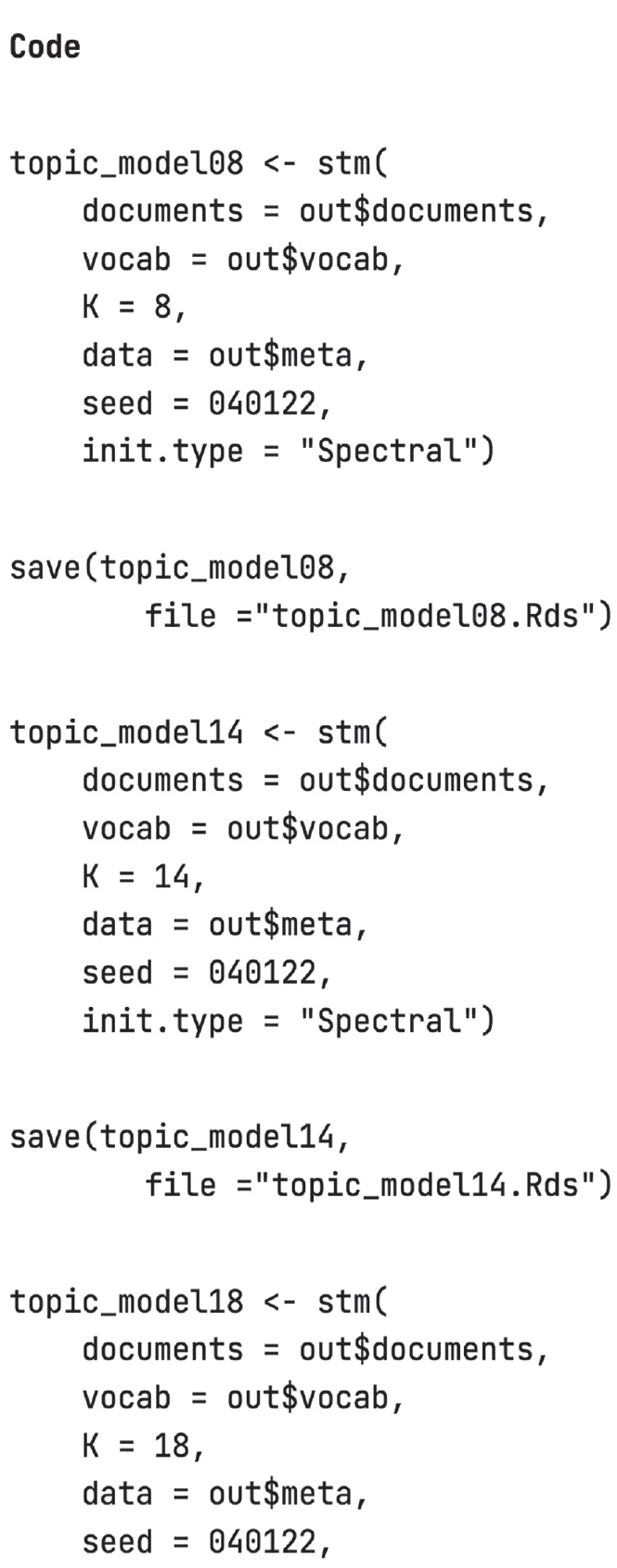
Code to fit models in full to the data. Be sure to save output objects for efficiency.

In comparing solutions, one might assess how representative individual topics are of the set of responses. This is calculated using the theta matrix from the model, which holds the per-document-per topic probabilities. In other words, values in the theta matrix represent the share of words in a document that are assigned to a topic; there is one value for each document–topic pair. Likelihoods in a document sum to 1, but more than one topic can have high likelihood of representing a response. In any given model, one may expect some topics to be common—that is, representing a large share of words in many documents—and for others to be rare—that is, representing a large share of words in few documents.

Researchers may wish to consider the degree to which a model generates such rare topics. Rare topics may carry important information, especially if they can help psychology researchers uncover unpopular opinions or underrepresented groups for study. For example, in the current study, relatively few mothers were pregnant, and their pregnancy-specific concerns appear only in a rare topic in Model-18 (see below). On the other hand, rare topics may have limited utility in statistical analyses. Specifically, analyses using rare topics (which will have low base rates) may suffer from floor effects, which can statistically bias coefficient estimates toward zero (Šimkovic & Träuble, 2019).

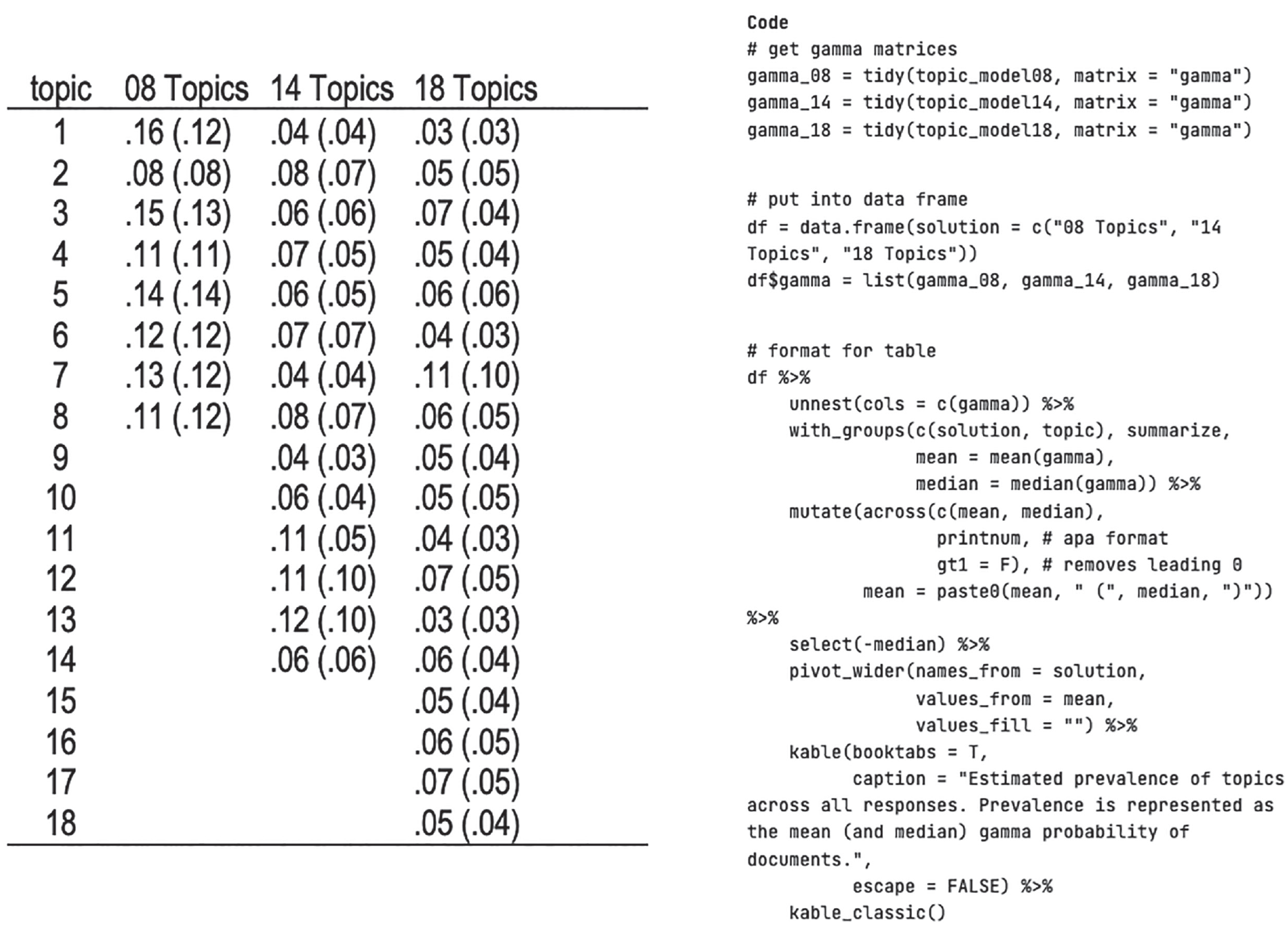
One way to evaluate the prevalence of topics is to estimate the frequency with which they dominate a document. This is most useful in cases in which documents are relatively short, such as the open-ended responses collected in the current study. The tidytext package provides an adapted version of the tidy() function that can extract the theta matrix from an stm object (see Fig. 4). Using this matrix, we identified for each document the topic that dominated, or the topic that covered the largest share of words in the document. We then counted for each topic the number of documents dominated. Comparing these frequencies in a model should make clear which topics are more rare. For example, the 18th topic (pregnancy-related issues) in Model-18 dominated only three of the documents.

Fig. 4.

Estimated prevalence of topics across all responses. Prevalence is represented as the mean (and median) theta probability of documents.

Solution congruence

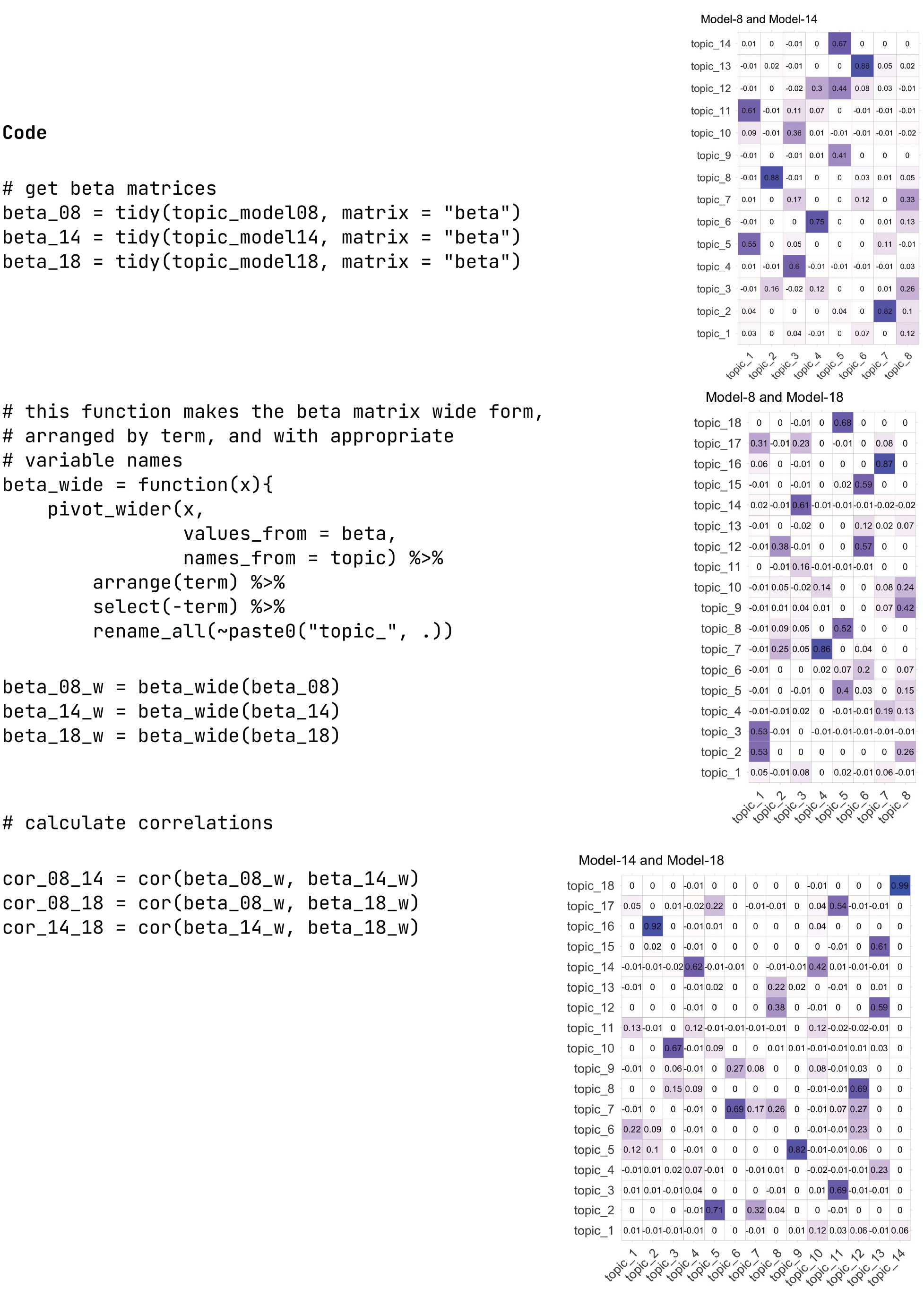
Researchers also examine the overlap in topics across solutions. Here, we used the beta matrix, which indicates the probability that each word was generated from each topic. One can then correlate beta weights across topics in different solutions to estimate the degree to which topics are overlapping. See Figure 5 for code to extract the beta matrices (again, using the tidytext package) and calculate congruence values. Correlations represent the congruence between two topics in terms of word probability. High values of congruence indicate high semantic overlap and may be indicative of robust topics. Figure 5 also includes visual representations of these matrices in the example data.

Fig. 5.

Estimating congruence across solutions. Values in boxes represent correlation between topics based on the beta matrices.

We recommend looking for topics with high correlations across solutions to identify themes that appear in all solutions. For example, one emerges in all three solutions (Topic 8-7, 14-2, and 18-16). Note that this topic represents a larger proportion of responses in Models-8 and -14. In the next section, on labeling topics, we pay particular attention to this theme. Alternatively, topics with low congruence across solutions may point to especially valuable models. That is, if one model is better able to extract an important idea from the corpus, it may be more useful than a model with more representative but less interesting topics.

Labeling topics

Labeling topics is a step necessary for the interpretation and further analysis of a topic model, but it can also provide qualitative support for selecting from a set of candidate models. Topic labeling can reveal that some topics are more relevant to a research question or, alternatively, reveal topics that are less informative. Especially in the case of many-topic solutions, differentiation between topics may reflect grammar rather than content (e.g., “have the vaccine” vs. “plan to get the vaccine”). Whether these grammatical differences are psychologically informative is up to the researcher, but only topic labeling can isolate such distinctions. In this section of the tutorial, we provide tools for identifying and labeling topics.³

Frequent and exclusive words

A relatively straightforward approach to identifying topic content is to examine the words most likely to be generated from that given topic or frequent words. A related but distinct set of words are exclusive words, which are not only frequent in the topic but also unlikely to appear in other topics. For example, the word “vaccine” is likely in many of the topics estimated with these data, but it does not always meet the threshold of exclusivity. The function labelTopics() from the stm package will extract both frequent and exclusive words for each topic in STM (Fig. 6). In some cases, it may be useful to display frequent and exclusive words graphically—this can be a useful method for quickly organizing and comparing topic content. The tidytext package allows researchers to quickly extract the beta matrix, and the resulting object is meant to integrate seamlessly with the tidyverse suite (Fig. 6).

Fig. 6.

Identifying frequent and exclusive words in topics. For this figure, we focus exclusively on Model-8, but for corresponding code and figures for the other candidate models, see the Supplemental Material available online.

Key examples

A second method for labeling topics is to examine key examples from the data set. Again, this is facilitated by a function in the stm package called “findThoughts()” (Fig. 7). This function will select the responses most likely to have been generated from each topic. Users can set the number of topics to examine (argument n). We also recommend setting a threshold for the smallest likelihood at which a response can be considered an exemplar (e.g., .3 or 30% for a model with relatively few topics or .05 for a model with many topics). This may result in fewer examples for some topics, but it prevents interpretation from becoming skewed by loosely affiliated responses.

Fig. 7.

Extracting key responses from topic model. Here we show how to extract the top responses for the fourth topic in Model-8. For more responses, see the Supplemental Material available online. We give an example here of extracting responses for multiple topics.

Correlations among topics

A final method to assist in the labeling of topics is to examine the correlations between topics. Previously, we used topic congruence—correlations across solutions—to compare candidate models; this allowed us to determine the extent to which a particular solution yielded different information. Here, we focus on correlations between topics in solutions. This method is especially useful when topics are difficult to label; identifying similar topics can help to clarify the meaning or themes.

The stm package includes the function topicCorr(), which estimates correlations between topics in a solution. (Note this differs from the solution-congruence analyses, which estimate correlations between topics across solutions.) Results from topicCorr() can be represented in a network figure that clearly depicts clusters among topics (Fig. 8). However, the plot function represents only positive correlations among topics—there may be meaningful negative correlations between topics not depicted. The Supplemental Material includes an example of a network figure representing both positive and negative correlations. Such an image may be less tidy but more accurately represent the correlations between figures.

Fig. 8.

Correlations between topics.

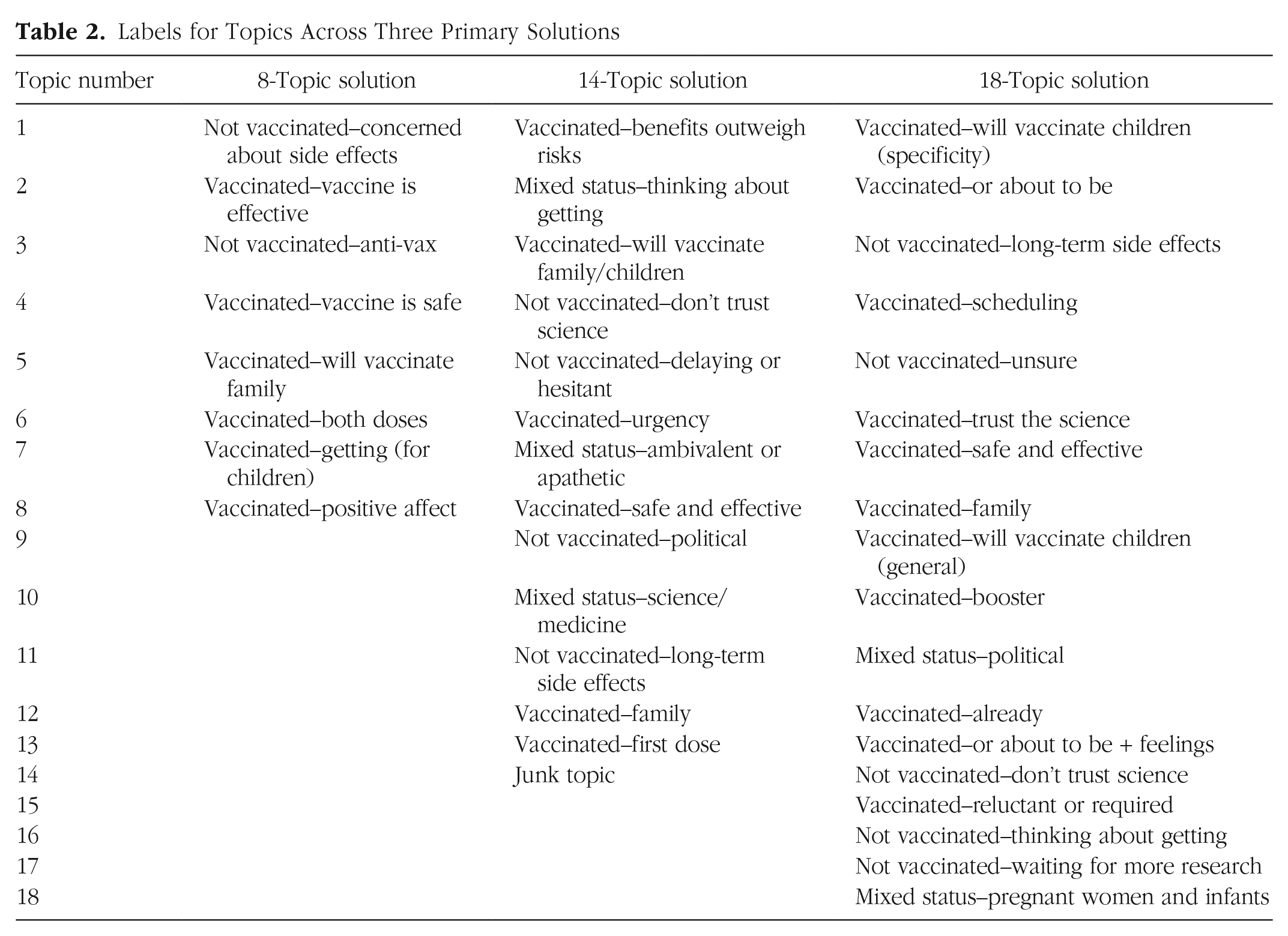
After considering frequent and exclusive words, key examples, and how topics cluster, S. J. Weston and I. Shryock independently generated and compared topic labels (see Table 2). These labels highlight several potential features of empirically derived topics. First, topics can be used to categorize. In our data, many of the topics identified vaccine status (e.g., fully vaccinated, first dose, planning to vaccinate, or not vaccinated). Although it is preferable to directly query vaccine status, this open-ended question allowed greater flexibility, especially as the types of vaccines available changed. Second, all solutions allowed us to differentiate participants on the basis of rationale for vaccinating, including their confidence in the vaccine. Third, several topics appear in multiple solutions—this is congruent with the cross-solution correlational analyses and is suggestive of themes or topics that are robust. Fourth, not all topics may be useful. Topic 14-14 was unidentified because the authors could not find a discernable theme in the key words or examples. The presence of uninterpretable topics does not necessarily mean a solution is not useful, although Maier et al. (2018) suggested removal of such topics from the final model.

Table 2.

Labels for Topics Across Three Primary Solutions

Topic number	8-Topic solution	14-Topic solution	18-Topic solution
1	Not vaccinated–concerned about side effects	Vaccinated–benefits outweigh risks	Vaccinated–will vaccinate children (specificity)
2	Vaccinated–vaccine is effective	Mixed status–thinking about getting	Vaccinated–or about to be
3	Not vaccinated–anti-vax	Vaccinated–will vaccinate family/children	Not vaccinated–long-term side effects
4	Vaccinated–vaccine is safe	Not vaccinated–don’t trust science	Vaccinated–scheduling
5	Vaccinated–will vaccinate family	Not vaccinated–delaying or hesitant	Not vaccinated–unsure
6	Vaccinated–both doses	Vaccinated–urgency	Vaccinated–trust the science
7	Vaccinated–getting (for children)	Mixed status–ambivalent or apathetic	Vaccinated–safe and effective
8	Vaccinated–positive affect	Vaccinated–safe and effective	Vaccinated–family
9		Not vaccinated–political	Vaccinated–will vaccinate children (general)
10		Mixed status–science/medicine	Vaccinated–booster
11		Not vaccinated–long-term side effects	Mixed status–political
12		Vaccinated–family	Vaccinated–already
13		Vaccinated–first dose	Vaccinated–or about to be + feelings
14		Junk topic	Not vaccinated–don’t trust science
15			Vaccinated–reluctant or required
16			Not vaccinated–thinking about getting
17			Not vaccinated–waiting for more research
18			Mixed status–pregnant women and infants

Discussion and Other Considerations

In this tutorial, we focused on identifying the number and content of topics when building structural topic models of open-ended survey responses. We described the process of preparing the data for analysis, selecting a wide range of solutions to consider, and narrowing that selection to a tractable number of candidates using fit statistics. Researchers may use all, some, or only one of these models in subsequent analysis. Moreover, topics that are robust to model selection (i.e., topics that appear regardless of the number of topics extracted) may be especially useful to researchers and potentially limit the need to choose a single model.

When choosing which models to evaluate in depth, researchers have a suite of tools available, including (a) evaluating topic depth in relation to project goals, (b) estimating the representativeness of topics in a corpus, and (c) comparing congruence across solutions. Labeling topics is also a necessary step both for choosing candidate models for evaluation and as an important analysis in and of itself. Labeling topics is facilitated by examining frequent and exclusive words, key examples, and the structure of topics in a solution. Although not discussed in this tutorial, a useful tool for assisting the comparison and labeling of topics is the stminsights package (Schwemmer, 2021).

Note that in the current tutorial, we focused mainly on quantitative metrics for determining the number of topics to estimate. However, topic modeling is not a technique that can be accomplished without the element of human interpretability. The goal of labeling topics, for example, is not only to identify themes but also to assess the validity and utility of a particular solution (i.e., number of topics). Bespoke approaches to topic interpretation and labeling (Ying et al., 2022), including crowdsourcing (Condon, 2017; Grimmer et al., 2022), are recommended.

Although outside the scope of this tutorial, we note additional considerations for topic modeling. A primary benefit of STM over other forms of topic modeling is the ability to include additional variables. These may include demographic, psychological, or other variables, such as time. The inclusion of additional variables is best integrated into the above analyses in the full estimation of topics (e.g., Fig. 3). Researchers can specify which variables they would associate with the prevalence of topics (using the prevalence argument) or the content of topics (using the content argument). Again, both the stm and tidytext packages include functions to facilitate examining the relationships of such variables to topics. We note here that the inclusion of additional variables may influence the results of a topic model—researchers are advised to include variables of interest from the start of the process described in this tutorial. As with all regression-type models, researchers should take care to avoid overfitting and multicollinearity.

Supplemental Material

sj-html-1-amp-10.1177_25152459231160105 – Supplemental material for Selecting the Number and Labels of Topics in Topic Modeling: A Tutorial

Supplemental material, sj-html-1-amp-10.1177_25152459231160105 for Selecting the Number and Labels of Topics in Topic Modeling: A Tutorial by Sara J. Weston, Ian Shryock, Ryan Light and Phillip A. Fisher in Advances in Methods and Practices in Psychological Science

Supplemental Material

sj-qmd-2-amp-10.1177_25152459231160105 – Supplemental material for Selecting the Number and Labels of Topics in Topic Modeling: A Tutorial

Supplemental material, sj-qmd-2-amp-10.1177_25152459231160105 for Selecting the Number and Labels of Topics in Topic Modeling: A Tutorial by Sara J. Weston, Ian Shryock, Ryan Light and Phillip A. Fisher in Advances in Methods and Practices in Psychological Science

Footnotes

Transparency

Action Editor: Yasemin Kisbu-Sakarya

Editor: David A. Sbarra

Author Contribution(s)

Sara J. Weston: Conceptualization; Formal analysis; Methodology; Writing – original draft.

Ian Shryock: Conceptualization; Formal analysis; Writing – original draft; Writing – review & editing.

Ryan Light: Methodology; Writing – review & editing.

Phillip A. Fisher: Conceptualization; Data curation; Methodology; Supervision; Writing – review & editing.

Correction (June 2023):

Article updated to include Open Data and Open Materials badges, as well as the Open Practices statement.

ORCID iD

Sara J. Weston

Supplemental Material

Additional supporting information can be found at

Notes

References

Airoldi

E. M.

Bischof

J. M.

(2016). Improving and evaluating topic models and other models of text. Journal of the American Statistical Association, 111(516), 1381–1403. https://doi.org/10.1080/01621459.2015.1051182

Banks

G. C.

Woznyj

H. M.

Wesslen

R. S.

Ross

R. L.

(2018). A review of best practice recommendations for text analysis in R (and a User-Friendly App). Journal of Business and Psychology, 33(4), 445–459. https://doi.org/10.1007/s10869-017-9528-3

Bedford-Petersen

Weston . (2021). Mapping individual differences on the internet: Case study of the type 1 diabetes community. JMIR Diabetes, 6(4), Article 30756. https://doi.org/10.2196/30756

Blei

D. M.

A. Y.

Jordan

M. I.

(2003). Latent Dirichlet allocation. Journal of Machine Learning Research, 3, 993–1022.

Blei

D. M.

Lafferty

J. D.

(2006). Dynamic topic models. In Cohen

W. W.

Moore

(Eds.), ICML ‘06: Proceedings of the 23rd international conference on machine learning (pp. 113–120). Association for Computing Machinery. https://doi.org/10.1145/1143844.1143859

Blei

D. M.

Lafferty

J. D.

(2007). A correlated topic model of science. The Annals of Applied Statistics, 1(1), 17–35.

Blei

D. M.

(2012). Probabilistic topic models. Communications of the ACM, 55(4), 77–84. https://doi.org/10.1145/2133806.2133826

Cattell

R. B.

(1966). The scree test for the number of factors. Multivariate Behavioral Research, 1(2), 245–276.

Condon

D. M.

(2017). The SAPA Personality Inventory: An empirically derived, hierarchically organized self report personality assessment model. PsyArXiv. https://doi.org/10.31234/osf.io/sc4p9

10.

Duncan

G. J.

Engel

Claessens

Dowsett

C. J.

(2014). Replication and robustness in developmental research. Developmental Psychology, 50(11), 2417–2425. https://doi.org/10.1037/a0037996

11.

Edelmann

Moody

Light

(2017). Disparate foundations of scientists’ policy positions on contentious biomedical research. Proceedings of the National Academy of Sciences, USA, 114(24), 6262–6267. https://doi.org/10.1073/pnas.1613580114

12.

Finch

W. H.

Hernández Finch

M. E.

McIntosh

C. E.

Braun

(2018). The use of topic modeling with latent Dirichlet analysis with open-ended survey items. Translational Issues in Psychological Science, 4(4), 403–424. https://doi.org/10.1037/tps0000173

13.

Zhuang

Zhu

Guo

(2021). Agreeing to disagree: Choosing among eight topic-modeling methods. Big Data Research, 23, Article 100173. https://doi.org/10.1016/j.bdr.2020.100173

14.

Grimmer

Roberts

M. E.

Stewart

B. M.

(2022). Text as data: A new framework for machine learning and the social sciences. Princeton University Press.

15.

Hvitfeldt

Silge

(2021). Supervised machine learning for text analysis in R. Chapman and Hall/CRC.

16.

Jackson

J. C.

Watts

List

J.-M.

Puryear

Drabble

Lindquist

K. A.

(2022). From text to thought: How analyzing language can advance psychological science. Perspectives on Psychological Science, 17(3), 805–826. https://doi.org/10.1177/17456916211004899

17.

Jeong

Yoon

Lee

J.-M.

(2019). Social media mining for product planning: A product opportunity mining approach based on topic modeling and sentiment analysis. International Journal of Information Management, 48, 280–290. https://doi.org/10.1016/j.ijinfomgt.2017.09.009

18.

Koltcov

Ignatenko

Koltsova

(2019). Estimating topic modeling performance with sharma–mittal entropy. Entropy, 21(7), Article 660. https://doi.org/10.3390/e21070660

19.

Lee

Mimno

(2017). Low-dimensional embeddings for interpretable anchor-based topic inference. ArXiv. https://doi.org/10.48550/arXiv.1711.06826

20.

Maier

Niekler

Wiedemann

Stoltenberg

(2020). How document sampling and vocabulary pruning affect the results of topic models. Computational Communication Research, 2(2), 139–152. https://doi.org/10.5117/CCR2020.2.001.MAIE

21.

Maier

Waldherr

Miltner

Wiedemann

Niekler

Keinert

Pfetsch

Heyer

Reber

Häussler

Schmid-Petri

Adam

(2018). Applying LDA topic modeling in communication research: Toward a valid and reliable methodology. Communication Methods and Measures, 12(2–3), 93–118. https://doi.org/10.1080/19312458.2018.1430754

22.

Mimno

Wallach

Talley

Leenders

McCallum

(2011). Optimizing semantic coherence in topic models. In Proceedings of the 2011 Conference on Empirical Methods in Natural Language Processing (pp. 262–272). Association for Computational Linguistics.

23.

Monroe

(n.d.). An introduction to the structural topic model. https://burtmonroe.github.io/TextAsDataCourse/Tutorials/IntroSTM.nb.html

24.

R Core Team. (2022). R: A language and environment for statistical computing [Manual]. https://www.R-project.org/

25.

Ramirez

E. H.

Brena

Magatti

Stella

(2012). Topic model validation. Neurocomputing, 76(1), 125–133.

26.

Rieger

Rahnenführer

Jentsch

(2020). Improving latent Dirichlet Allocation: On reliability of the novel method LDA prototype. In Métais

Meziane

Horacek

Cimiano

(Eds.), Natural language processing and information systems (pp. 118–125). Springer International Publishing. https://doi.org/10.1007/978-3-030-51310-8_11

27.

Roberts

M. E.

Stewart

B. M.

Tingley

(2019). stm: An R package for structural topic models. Journal of Statistical Software, 91(2), 1–40. https://doi.org/10.18637/jss.v091.i02

28.

Roberts

M. E.

Stewart

B. M.

Tingley

Lucas

Leder-Luis

Gadarian

S. K.

Albertson

Rand

D. G.

(2014). Structural topic models for open-ended survey responses. American Journal of Political Science, 58(4), 1064–1082. https://doi.org/10.1111/ajps.12103

29.

Schmiedel

Müller

vom Brocke

(2019). Topic modeling as a strategy of inquiry in organizational research: A tutorial with an application example on organizational culture. Organizational Research Methods, 22(4), 941–968. https://doi.org/10.1177/1094428118773858

30.

Schofield

Mimno

(2016). Comparing apples to apple: The effects of stemmers on topic models. Transactions of the Association for Computational Linguistics, 4, 287–300.

31.

Schwemmer

(2021). stminsights: A “shiny” application for inspecting structural topic models [Manual]. https://github.com/cschwem2er/stminsights

32.

Silge

(2018, September 8). Training, evaluating, and interpreting topic models. Julia Silge. https://juliasilge.com/blog/evaluating-stm/

33.

Silge

Robinson

(2016). tidytext: Text mining and analysis using tidy data principles in R. Journal of Open Source Software, 1(3), Article 37. https://doi.org/10.21105/joss.00037

34.

Šimkovic

Träuble

(2019). Robustness of statistical methods when measure is affected by ceiling and/or floor effect. PLOS ONE, 14(8), Article e0220889. https://doi.org/10.1371/journal.pone.0220889

35.

Steegen

Tuerlinckx

Gelman

Vanpaemel

(2016). Increasing transparency through a multiverse analysis. Perspectives on Psychological Science, 11(5), 702–712.

36.

Taddy

(2012). On estimation and selection for topic models. In Proceedings of the Fifteenth International Conference on Artificial Intelligence and Statistics, PMLR 22, 1184–1193.

37.

Valdez

Pickett

A. C.

Goodson

(2018). Topic modeling: Latent semantic analysis for the social sciences. Social Science Quarterly, 99(5), 1665–1679. https://doi.org/10.1111/ssqu.12528

38.

Wallach

H. M.

(2006). Topic modeling: Beyond bag-of-words. In Proceedings of the 23rd International Conference on Machine Learning (pp. 977–984). Association for Computing Machinery.

39.

Warin

(n.d.). Visualize: Presenting STM results. https://warin.ca/shiny/stm/#section-visualize

40.

Wicherts

J. M.

Veldkamp

C. L.

Augusteijn

H. E.

Bakker

Van Aert

Van Assen

M. A.

(2016). Degrees of freedom in planning, running, analyzing, and reporting psychological studies: A checklist to avoid p-hacking. Frontiers in Psychology, 7, Article 1832. https://doi.org/10.3389/fpsyg.2016.01832

41.

Wickham

Averick

Bryan

Chang

McGowan

L. D.

François

Grolemund

Hayes

Henry

Hester

Kuhn

Pedersen

T. L.

Miller

Bache

S. M.

Müller

Ooms

Robinson

Seidel

D. P.

Spinu

. . . Yutani

(2019). Welcome to the tidyverse. Journal of Open Source Software, 4(43), Article 1686. https://doi.org/10.21105/joss.01686

42.

Ying

Montgomery

J. M.

Stewart

B. M.

(2022). Topics, concepts, and measurement: A crowdsourced procedure for validating topics as measures. Political Analysis, 30(4), 570–589. https://doi.org/10.1017/pan.2021.33

Supplementary Material

Please find the following supplemental material available below.

For Open Access articles published under a Creative Commons License, all supplemental material carries the same license as the article it is associated with.

For non-Open Access articles published, all supplemental material carries a non-exclusive license, and permission requests for re-use of supplemental material or any part of supplemental material shall be sent directly to the copyright owner as specified in the copyright notice associated with the article.

0.00 MB

0.17 MB

0.04 MB