Sage Journals: Discover world-class research

Abstract

Factorial designs are common in psychology research. But they are nearly always used without control of the experiment-wise Type I error rate (EWER), perhaps because of a lack of awareness about viable procedures for that purpose and perhaps also because of a lack of appreciation for the problem of Type I error inflation. In this article, key concepts relating to Type I error inflation are discussed, with emphasis on the 2 × 2 factorial design. Simulations are used to evaluate various approaches in that context. I show that conventional approaches often do not control the EWER. Alternative approaches are recommended that reliably control the EWER and are simple to implement.

Keywords

ANOVA alpha error rate error Type 1 error multiplicity open materials

The purpose of null hypothesis testing is to control the Type I error rate. When there is only one effect to test, Type I error control is fairly straightforward: Provided that statistical assumptions are met, the maximum Type I error rate is simply the α level chosen for the test (conventionally .05). However, when more than one inference is made in an analysis, there is a multiple comparisons problem (sometimes called multiple testing or multiplicity). That is, the “overall” Type I error rate for the analysis can be considerably higher than the α levels of the individual tests (the comparison-wise α levels). Exactly how high the overall Type I error rate is depends in part on how it is defined. The main ways to define the overall Type I error rate are the following:

Per-family Type I error rate (PFER; Tukey, 1953). The PFER is the a priori expected number of Type I errors that will occur in a family, where the family is the set of tests under consideration. In other words, the PFER is the sum of the Type I error rates of all the individual tests. For instance, if a family consists of two tests of true null hypotheses, each conducted at .05, then the PFER is .05 + .05 = .1. The PFER can be controlled at α (the designated maximum overall Type I error rate) using the Bonferroni procedure: Each comparison-wise α level is set to α / m, where α is the designated overall α level and m is the number of tests. For instance, if a family consists of two tests, then setting the comparison-wise α level at .05 / 2 = .025 caps the PFER at .025 + .025 = .05. The PFER can be called the per-experiment Type I error rate (PEER) when the family consists of all the tests of interest in an investigation.

Familywise Type I error rate (FWER; Tukey, 1953). The FWER is the a priori probability of at least one Type I error occurring in the family of tests. Note that the phrase “at least one Type I error” does not distinguish between one Type I error and multiple Type I errors. Thus, whereas the PFER tallies every Type I error that occurs, the FWER does not count multiple co-occurring Type I errors as any “worse” than a single Type I error. Consequently, FWER control is less strict than PFER control. That is, the FWER is always less than or equal to the PFER. Thus, the Bonferroni procedure is conservative (i.e., overly stringent) when the goal is merely to control the FWER. There are less stringent adjustments that have greater statistical power (i.e., they allow effects to be statistically significant with greater frequency). But that power advantage can be achieved only by sacrificing strict PFER control.

Experiment-wise Type I error rate (EWER; Tukey, 1953). The EWER is simply another name for the FWER when the family consists of all the tests of interest in an investigation. The terms EWER and FWER are often used interchangeably under the assumption that typically they are indeed equivalent. However, researchers sometimes divide a single experiment’s tests into multiple distinct families, so the two terms are not interchangeable in all contexts (see Sheskin, 2007, p. 1137).

False discovery rate (FDR; Benjamini & Hochberg, 1995). Loosely speaking, the FDR is the a priori expected proportion of significances in the family that will be Type I errors. That is, the FDR is the expected false discovery proportion. FDR control is less strict than FWER control. That is, the FDR is always less than or equal to the FWER. Use of the FDR is typically reserved for situations involving very large numbers of tests, such as when screening thousands of genetic variants in a genome-wide association study. The rationale for using this less stringent form of Type I error control in such cases is presumably that a few Type I errors per study are tolerable if those errors are accompanied by numerous “true discoveries” (statistically significant tests of real effects).

Each of the above definitions of the overall Type I error rate can be conceptualized as a frequency of Type I errors among infinite theoretical iterations of an experiment. In Figure 1, each of the 20 columns of boxes represents a family of four tests for a given iteration of an experiment. Test A is of a false null hypothesis. Tests B, C, and D are of true null hypotheses. Assume that those tests constitute all the tests of interest in the experiment, so PEER = PFER and EWER = FWER. Black boxes represent Type I errors, gray boxes represent true discoveries, and white boxes represent nonsignificances. Assume that the frequencies of those outcomes in this set of 20 iterations are equal to the theoretical frequencies from infinite iterations. In these 20 iterations, there are three Type I errors altogether (two in Iteration 8 and one in Iteration 14), so PFER = 3 / 20 = .15. In two of the 20 iterations (specifically, Iterations 8 and 14), there is at least one Type I error, so FWER = 2 / 20 = .1. The false discovery proportion is two thirds in Iteration 8 (because there are three significances, two of which are Type I errors), is one half in Iteration 14 (because there are two significances, one of which is a Type I error), and is zero in the other 18 iterations (because the false discovery proportion is considered as zero in any iteration with no false discoveries even when there are no true discoveries either). The FDR is the expected value (i.e., the mean) of those false discovery proportions, so FDR = (2/3 + 1/2 + 18 × 0) / 20 ≈ .058. Thus, by all definitions, the overall Type I error rate is inflated above .05. But the Type I error rate for each individual test of a true null hypothesis remains 1 / 20 = .05. Incidentally, Figure 1 also shows the statistical power of Test A: There are 16 true discoveries out of 20 iterations, so the power of the test is 16 / 20 = .8.

Fig. 1.

Theoretical iterations of an experiment with a family of four null hypothesis tests.

Note that the PFER counts all three Type I errors in those iterations, whereas the FWER essentially allows the two co-occurring errors in Iteration 8 to count as a single error. Indeed, the more that Type I errors tend to co-occur, the larger the difference is between the FWER and the PFER. For instance, when tests are positively correlated, Type I errors are more likely to co-occur. That does not affect the PFER, but it makes the FWER lower. Thus, when there is some inherent correlation between tests, the FWER can be controlled with less stringent adjustments. For example, when performing pairwise comparisons and each cell is involved in more than one comparison, the FWER can be controlled using specialized pairwise-comparison procedures that exploit the inherent correlation between tests that have a cell in common. There are also FWER-control procedures that are more general purpose in that they can be applied to a variety of multiple-testing situations, not just to pairwise comparisons. For instance, Holm’s (1979) procedure makes no assumptions about intertest correlation and instead uses a conditional testing structure to increase the concurrence of Type I errors. Some other FWER-control procedures assume nonnegative intertest correlation, which is generally a safe assumption for two-sided tests. For instance, the Šidák (1967) procedure, which is optimized for independent tests and is only marginally less stringent than the Bonferroni procedure, sets each comparison-wise α level to 1 − (1 − α)^1/m.

The 2 × 2 Design

The 2 × 2 experimental design, which has two factors with two levels each, is common in experimental research. And because it is the simplest factorial (i.e., multifactor) design, it is often the first factorial design that is taught. As diagrammed in Figure 2, there are four population means of interest in a 2 × 2 design: µ₁₁, µ₁₂, µ₂₁, and µ₂₂, where each µ is the population mean for a given cell, the first subscripted digit denotes the level of Factor A, and the second subscripted digit denotes the level of Factor B.

Fig. 2.

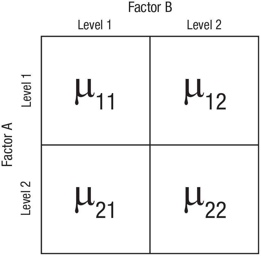
Population cell-means in a 2 × 2 design.

Tests of the simple effects (pairwise between-cells differences) in a 2 × 2 design are often limited to the pairwise comparisons between cells that have one factor level in common (i.e., comparisons across each row and across each column in the 2 × 2 layout). In such cases, the null hypotheses of interest are µ₁₁ = µ₁₂, µ₁₁ = µ₂₁, µ₁₂ = µ₂₂, and µ₂₁ = µ₂₂. In other situations, the researcher might be interested in all six pairwise comparisons. For instance, consider the case in which each factor is a treatment (active vs. placebo). The researcher may want to evaluate how undergoing the two treatments in combination compares with undergoing neither treatment and how undergoing Treatment A but not Treatment B compares with undergoing Treatment B but not Treatment A. In such cases, the null hypotheses for the “diagonal” comparisons would be of interest: µ₁₁ = µ₂₂ and µ₁₂ = µ₂₁.

In classical 2 × 2 analysis of variance (ANOVA), three other null hypotheses are defined: main effect of Factor A (µ₁₁ + µ₁₂ = µ₂₁ + µ₂₂), main effect of Factor B (µ₁₁ + µ₂₁ = µ₁₂ + µ₂₂), and interaction of the two factors (µ₁₁ − µ₁₂ = µ₂₁ − µ₂₂). In simple terms, a main effect is one factor’s effect “on average,” collapsing across both levels of the other factor. And the interaction is the extent to which a given factor’s effect differs between levels of the other factor. In other words, if there is an interaction, the two factors combine in a nonadditive way. A familiar example is drug interaction: Drug A may have little effect on its own but may enhance, neutralize, or reverse the effect of Drug B.

If the null hypothesis for the interaction is false (i.e., if there is a real interaction in the population), that means the magnitude—and perhaps even the direction—of each factor’s effect depends on the level of the other factor. In that case, the simple effects of a given factor cannot be thoroughly described by collapsing them into a single main effect. But if the null hypothesis for the interaction is true (i.e., if there is no interaction in the population), that means that the effect of a given factor does not differ between levels of the other factor. In that case, the two simple effects of a given factor are equivalent and thus can be more simply described by collapsing them into a single main effect. Hence, testing main effects may be considered a more efficient way of testing simple effects in the special case of no interaction.

The problem is that the researcher does not actually know whether the null hypothesis for the interaction is true and thus does not know for certain whether main-effect tests are sufficient. Therefore, a classical approach is to conduct a null hypothesis test of the interaction and then treat that null hypothesis as true if it is not rejected by the test. That is, the researcher tests the four simple effects if the interaction is statistically significant and tests the two main effects if the interaction is nonsignificant (Bethea et al., 1995, p. 233; Bobko, 1986; Devore, 1987, pp. 413–414; Heiberger & Holland, 2004, p. 338; Hochberg & Tamhane, 1987, p. 294; Howell, 2013, p. 420; Nestor & Schutt, 2012, p. 218; Shaffer, 1991; Tamhane, 2009, pp. 232–233; Weber & Skillings, 2000, pp. 429–430). With this approach, a significant interaction test would not typically be claimed as a discovery in itself (although it might be). Rather, the interaction test functions like a railroad track switch that determines whether the analysis goes down the “main-effect track” or the “simple-effect track.” In the present article, we refer to this approach as the two-track testing structure.

A problem with the two-track testing structure is that because of limited statistical power of the interaction test, analyses may often go down the main-effect track even when the interaction is nonzero in the population. This can lead to somewhat meaningless analyses. For example, consider the case in which one factor is a treatment and the other factor is the sex of the patient. If the treatment effect substantially differed between males and females, then simply describing the effect of the treatment “on average” would not accurately describe the treatment effect in patients of either sex. In theory, the main effect of treatment might even be driven entirely by an effect in one sex. In that case, misinterpreting a significant main effect of the treatment as implying a treatment effect in both males and females would be a “de facto Type I error”—even though the main effect itself would not be a Type I error per se. Given these concerns, it may often be better to forgo the main-effect tests altogether and decide a priori to use a “one track” approach that tests only the simple effects.

The Overall Type I Error Rate in 2 × 2 Designs

Because there is more than one test in the 2 × 2 design, there is a potential multiple-comparisons problem. But how should the overall Type I error rate be defined?

Because of the relatively small number of tests in a 2 × 2 design, FDR is not likely to be the most relevant definition in most cases (but see “Remedy 3” described by Cramer et al., 2016). Moreover, FDR control is generally not considered sufficiently rigorous for confirmatory inferences (Tamhane, 2009, p. 128), although it is of course more rigorous than disregarding the multiple-comparisons problem altogether.

A few authors have argued that PFER is often the most relevant definition of the overall Type I error rate. For example, it has been noted that settling for FWER control comes with the dubious implication that multiple errors are no worse than one (Barnette & McLean, 2005; Frane, 2015a; Lawrence, 2019; Spjøtvoll, 1972). Moreover, controlling the PFER always controls the FWER, whereas controlling the FWER does not necessarily control the PFER. To control the PFER in the 2 × 2 design, one would simply apply the Bonferroni procedure to all the tests of interest.

Nonetheless, the FWER appears to have beaten out the PFER as the preferred standard among researchers. The vast number of FWER-control procedures that have been devised over the past several decades and the vast number of textbooks that mention the FWER but not the PFER are testaments to that verdict (Frane, 2015a). On the other hand, the Bonferroni procedure remains in widespread use, which means that researchers are often implementing PFER control even if they refer to the Bonferroni procedure only as an FWER-control method and do not realize the additional level of control it provides.

If one accepts FWER as the preferred definition of the overall Type I error rate, then the task of defining the family still remains. An obvious approach would be to define the family as the set of all the tests of interest in the experiment, in which case FWER = EWER. Klockars et al. (1995) argued that including multiple factors in the same experiment inherently implies that the effects of those factors are being evaluated jointly as a single family. Likewise, Miller’s (1981, p. 34) classic text on multiple comparisons noted that—heuristically speaking—the “natural family” typically consists of the tests for a “single experiment” (see also Ryan, 1962; Westfall & Young, 1993, p. 220). Note that Miller included two-way (i.e., two-factor) ANOVA as an example of a single experiment. However, Miller also rightly acknowledged that defining families is subjective and that the appropriate definition depends on the “problem at hand” (p. 35).

It makes sense to exclude a test from the family if significance in that test would not constitute a publishable discovery and would not constitute a basis for decision-making in itself. For instance, imagine a 2 × 2 study of treatment efficacy in which the factor of primary interest is a treatment and the second factor is the sex of the patient. The goal of the study would presumably be to demonstrate an effect of treatment in each sex, not to demonstrate an effect of sex, so it would likely be inappropriate to adjust the tests of primary interest to account for any sex-effect tests.

I am inclined to agree with Miller (1981) that the natural way to define the family is to include all the tests in the experiment unless there is a specific reason—declared a priori—that the problem at hand calls for some other definition. But in practice, EWER control is rarely applied in 2 × 2 designs (or in factorial designs more generally), as discussed in the next section.

Conventional Approaches to Type I Error Control in Factorial Designs

No adjustment

Often in factorial designs, no multiple-testing adjustment is performed. In fact, Cramer et al. (2016) reviewed the statistical analyses in six well-known psychology journals and found that although nearly half of the articles used a factorial ANOVA, only 1% of those ANOVA-based analyses addressed the multiple-comparisons problem in any way. That is, 99% of the articles did not attempt to control the Type I error rate at any level beyond the individual comparison level (although Cramer et al. appear to have focused on the main-effect and interaction tests, and it is not clear how simple effects were typically evaluated in the studies they examined).

Why is failure to adjust for multiple comparisons so common? The simplest explanation may be that researchers want to find statistical significance and thus are not inclined to do anything that would reduce the statistical power of their tests. As noted by Luck and Gaspelin (2017), “there is a tension between the short-term desire of individual researchers to publish papers and the long-term desire of the field as a whole to minimize the number of significant but bogus findings in the literature” (p. 149).

Often the decision not to adjust for multiple comparisons is rationalized using the idea that “planned comparisons” (i.e., tests that were planned a priori) are inherently exempt from adjustment. That misconception was critiqued in detail by Frane (2015b) and was ridiculed by Steinfatt (1979), who satirically described an EWER-control procedure that consisted solely of chanting “I plan thee, I plan thee, I plan thee” over each test. Although it is true that failing to plan the tests exacerbates the multiple-comparisons problem, that does not imply that planning the tests eliminates the multiple-comparisons problem. Adjusting for multiple comparisons may not even be possible when tests are unplanned because the number of tests to adjust for may become indeterminate, especially when subgroup analyses and transformations are considered. Thus, planning the analysis is not a special circumstance that makes multiple-testing adjustment unnecessary. On the contrary, planning the analysis is part of the standard scientific procedure that makes confirmatory inferences valid and makes multiple-testing adjustments effective.

Omnibus protection

In omnibus protection (first proposed by Fisher, 1935, Section 24), the first step is to conduct an omnibus test at α. This test evaluates the joint null hypothesis of no main effects and no interaction, which is equivalent to the hypothesis that all population means are equal. If the omnibus test is significant, then all tests of interest are conducted at α without adjustment. And if the omnibus test is nonsignificant, then significance of all tests is forfeited. Thus, the omnibus test functions as a “gatekeeper” that determines whether further tests are allowed.

The rationale for this approach is that when all population means are equal, the omnibus test is significant only with probability α. Consequently, when all population means are equal, the probability of Type I error in one or more tests of interest cannot exceed α because the probability of getting to conduct those tests at all is α. The problem is that when using omnibus protection, the maximum EWER does not occur when all population means are equal but rather when only some population means are equal (Kromrey & Dickinson, 1995). For instance, imagine that µ₁₁ = µ₁₂ << µ₂₁ = µ₂₂ and that there are four simple effects of interest (the two row effects and the two column effects). In that case, there is a large main effect of Factor A, making the power of the omnibus test very high. That neutralizes the omnibus protection for the simple-effect tests of the two true null hypotheses (µ₁₁ = µ₁₂ and µ₂₁ = µ₂₂). Or imagine that µ₁₁ = µ₁₂ = µ₂₁ << µ₂₂ and that all six simple-effect tests are of interest. In that case, there are two large main effects and a large interaction, so the power of the omnibus test is very high. That neutralizes the omnibus protection for the simple-effect tests of the three true null hypotheses (µ₁₁ = µ₁₂ and = µ₁₁ = µ₂₁ and µ₁₂ = µ₂₁).

Thus, omnibus protection controls the EWER only “in the weak sense” (Hochberg & Tamhane, 1987, p. 3). That is, it controls the EWER when all null hypotheses are true but not when only some null hypotheses are true.

Leaving the main-effect tests unadjusted

In some cases, the tests of interest are divided into separate families. FWER control is then applied to each family individually, leaving the overall EWER uncontrolled. Toothaker (1993) observed that in two-way ANOVA, “most researchers choose to control α for each of the three families of comparisons: the main effect means for A, the main effect means for B, and the cell means” (p. 79; see also Cardinal & Aitken, 2006; Devore, 1987, pp. 417–418; Girden, 1992, pp. 39–40; Gonzalez, 2009, p. 340; Hancock & Klockars, 1996, p. 276; Hays, 1988, p. 458; Huberty & Morris, 1988; Maxwell et al., 2018, p. 218; Miller, 1981, p. 35; Shaffer, 1995; Tamhane, 2009, pp. 232–233, 242; Weber & Skillings, 2000, pp. 430–431). In fact, that is the approach facilitated by IBM SPSS.

Note that in the 2 × 2 case, treating each main effect as its own family means that no adjustment is applied to the main-effect tests because there is only one comparison for each main effect. Of course, adjusting the simple-effect tests and not the main-effect tests would not inflate the EWER if the simple-effect tests were the only tests of interest. But if there were any a priori potential for the main effects to be tested—as is the case when using the two-track approach—then exempting the main-effect tests from adjustment could inflate the EWER.

The tradition of forgoing adjustment for main-effect tests may have endured in part because of the long-standing popular belief that any small number of tests is exempt from adjustment if they are orthogonal. Although the main-effect tests are not orthogonal to the corresponding simple-effect tests, they are approximately orthogonal to each other and to the interaction test. As noted by Hays (1988), “current practice tends to ignore the familywise error rate in carrying out a fairly small number of tests that can be regarded as (more or less) independent, as with a set of planned orthogonal comparisons” (p. 411; see also Brown & Melamed, 1990, p. 27; Cohen et al., 2003, p. 184; Kirk, 2013, p.178; and many others). But there appears to be no legitimate basis for exempting orthogonal tests from adjustment (Frane, 2015b; Klockars et al., 1995; Ludbrook, 1991). In fact, orthogonal tests produce higher EWERs than positively correlated tests (all other things being equal). And even for just two orthogonal tests, the EWER when the null hypotheses are true is nearly twice the comparison-wise α level. Assuming a comparison-wise α level of .05, that means that if both main effects were zero in the population, then failing to adjust the main-effect tests would give the researcher a nearly one in 10 chance of claiming a discovery that was spurious—even if no other tests were considered.

Disregarding the simple effects

Some approaches control the EWER but do not consider the simple effects. Such methods either test only the main effects or only the interaction and main effects (e.g., Cramer et al., 2016; Small et al., 2011; Williams, 1973). The usefulness of such methods is likely to be very limited. Main effects often do not adequately address the research question. And reporting a significant interaction without providing details about how the cell means differ is typically not sufficient to support a decision or interesting claim (Bibby, 2012). Although simple-effect testing is not the only way to follow up on a significant interaction (Rosnow & Rosenthal, 1989), it is typically the most straightforward and informative way (Howell, 2013, p. 420; Toothaker, 1993, p. 79), especially in the simple 2 × 2 case.

Viable Methods of EWER Control in Factorial Designs

A method is considered to be “viable” in the present article if it controls the EWER and does not substitute main-effect tests for simple-effect tests. The methods described in this section achieve their power by exploiting either intertest correlation, conditional testing structures (i.e., allowing significance in one test to affect significance in other tests), or both.

Simulation-based adjustment (the α_C method)

Recall that when tests are positively correlated, the EWER can be controlled using less stringent adjustments. In some cases, computing the optimal comparison-wise α-level adjustment can be done analytically (e.g., Dunnett, 1955; Tukey, 1953). In other cases, that computation is intractable (e.g., when cell sizes are unequal and intertest correlations are complex), but the optimal adjustment can be determined by simulation. The idea of using simulation to determine comparison-wise α-level adjustments is not new (e.g., see Edwards & Berry, 1987; Hsu & Nelson, 1998; Westfall et al., 2011, pp. 87–90). But it does not appear to be commonly applied in factorial designs. The process consists of the following steps.

First, use random number generation to simulate data from millions of theoretical iterations of the experiment that the researcher plans to conduct—iterations such as represented in Figure 1, except with millions of iterations instead of 20. These simulations use “worst case” parameter values that maximize the EWER (e.g., typically all populations means are set to be equal). And second, find an adjusted comparison-wise α level (α_C) that produces an estimated EWER equal to α. In other words, if α_C is applied to the tests of interest in all iterations, then the proportion of iterations that produce at least one Type I error should be α.

Once a tabulated value of α_C is available for a given design, researchers do not actually have to conduct the simulations. They can just look up the value in a table. See the Appendix for tabulated values of α_C in balanced 2 × 2 designs with four tests of interest (i.e., the two-row simple effects and the two-column simple effects) and with six tests of interest (all pairwise comparisons). Note that for a between-subjects design with any sample size, the value of α_C is approximately .014 for four tests and approximately .010 for six tests. Values of α_C for cell-size configurations not included in the tables can be obtained using the R programs provided in the Supplemental Material available online.

Hommel procedure

The Hommel (1988) procedure is a general-purpose multistep method of FWER control, similar to the Holm (1979) and Hochberg (1988) procedures but with more statistical power. It uses the following algorithm, where α is the experiment-wise α level, m is the number of tests, {p₍₁₎, . . . , p_(m)} are the p values for those tests (ordered from smallest to largest), and b is the integer vector {1, . . . , m}:

Sequentially, for each value of b from 1 to m, if p_{(m − j + 1)} < (b − j + 1) α / b for any j = {1, . . . , b}, then {p₍₁₎, . . . , p_{(m − b + 1)}} are significant, any other p values are nonsignificant, and the procedure stops. Else, the procedure continues to the next value of b; or if b has been exhausted, the procedure stops, and all p values are nonsignificant.

That conditional testing structure allows the Hommel procedure to capitalize on co-occurring Type I errors. For instance, consider a family of two tests in which both p values are only nominally less than α = .05. Neither p value would be significant with the classical Bonferroni procedure. But the Hommel procedure declares both p values significant without risking inflation of the FWER. To understand how, consider the two possibilities: (a) If the first p value reflects a real effect, then the only chance of Type I error is in the second test, so the full α can be “spent” on the second test, and (b) if the first p value does not reflect a real effect, then there is already a Type I error in the first test, making the second test inconsequential to the FWER (because the FWER does not distinguish one error from multiple errors). Therefore, when there are two tests, the Hommel procedure allows both p values to be significant if the larger p value is < .05. Only when the larger p value is > .05 is a reduced comparison-wise α level of .025 used for the second p value. When there are more than two tests, the computation becomes more complex, but the basic principle is the same. Because reporting multiple different comparison-wise α levels may be cumbersome, the Hommel procedure is typically applied as a p-value adjustment, which can be done with one simple command in R, using the p.adjust function.

Single-step all-possible-pairs methods

In some cases, the researcher is interested in comparing all possible pairs (e.g., testing all six simple effects in a 2 × 2 design). Numerous EWER-control procedures have been devised that exploit the inherent intertest correlations in the all-possible-pairs case. But such procedures are rarely applied to all cells in a factorial design. And IBM SPSS currently facilitates such application only if the cells are restructured into a one-way layout.

One of the best known all-possible-pairs methods is the Tukey–Kramer procedure (Kramer, 1956), which generalizes Tukey’s (1953) classical honest significant difference procedure to accommodate unequal cell sizes. Because Tukey–Kramer uses the omnibus error term for the pairwise comparisons, it assumes equal variance across all cells, putting the validity of the procedure at risk when variances are unequal (as they often are in nature). To avoid that risk, several alternative procedures have been developed to accommodate unequal variances. Among those procedures, Games–Howell (Games & Howell, 1976), Dunnett’s C (Dunnett, 1980), and Dunnett’s T3 (Dunnett, 1980; an improvement of Tamhane’s T2, Tamhane, 1979) are commonly recommended (Hochberg & Tamhane, 1987; Ramsey et al., 2011; Sauder & DeMars, 2019).

Other commonly available methods

Statistical software packages, such as IBM SPSS, offer additional multiple-testing procedures, such as Bonferroni, Šidák, and Scheffé. But the Bonferroni procedure is optimized for PFER/PEER control and thus is conservative for FWER/EWER control. The Šidák procedure is only marginally more powerful than Bonferroni and, because it is optimized for independent tests, does not exploit the intertest correlations that are inherent to pairwise comparisons. The Scheffé procedure is often the most conservative of all because it is designed to accommodate not only all possible pairs but also all possible linear combinations (which are likely not of interest in most cases).

Protected adjustment

Recall that omnibus protection alone does not control the EWER in factorial designs. However, it does provide control in the case that all population means are equal. Therefore, complete EWER control can be achieved by supplementing omnibus protection with adjustments that control the EWER when not all population means are equal. That way, the omnibus protection handles the all-means-equal case, the adjustment handles all other cases, and together the two techniques control the EWER in all cases (Levin et al., 1994; Shaffer, 1986).

When four simple effects are of interest

Consider the null hypotheses for the two-row simple effects and the two-column simple effects in the 2 × 2 design. If not all means are equal, then at most, two of those four null hypotheses can be true. For instance, if all means are equal except µ₁₁, then the only true null hypotheses are the two that do not involve µ₁₁ (i.e., µ₁₂ = µ₂₂ and µ₂₁ = µ₂₂). Therefore, if omnibus protection is used, the adjustments of the four simple-effect tests need to be only stringent enough to account for two null hypotheses. Specifically, each simple effect can be tested at α / 2 (i.e., what the Bonferroni adjustment would be for three tests) or at the marginally less stringent level 1 − (1 − α)^1/2 (i.e., what the Šidák adjustment would be for two tests). In the present article, I refer to the latter adjustment as the Šidák–Fisher procedure because it combines the Šidák adjustment with Fisher’s omnibus protection. Šidák–Fisher is optimized for independent tests, so it provides exact EWER control in the worst case: no correlation between the tests of true null hypotheses (e.g., when µ₁₁ = µ₁₂ ≠ µ₂₁ = µ₂₂).

When six simple effects are of interest

If all six pairwise tests are of interest and not all means are equal, then at most three of the six null hypotheses can be true. In fact, if all six pairwise tests plus the interaction test are of interest, then at most three of the seven null hypotheses in that family can be true. Therefore, if omnibus protection is used, then the six simple-effects tests and the interaction can each be tested at α / 3 (i.e., what the Bonferroni adjustment would be for three tests) or at the marginally less stringent level 1 − (1 − α)^1/3 (adapting the Šidák–Fisher adjustment that was described earlier).

Slightly more power in the protected tests can be achieved by exploiting the intertest correlations because no three of the tests can be independent. For instance, if omnibus protection is used in the between-subjects case, then the six simple effects can be tested using the equivalent of what the Tukey–Kramer adjustment would be for three tests. That approach (i.e., omnibus protection combined with what the Tukey–Kramer adjustment would be for one less than the number of groups) is known as the Hayter–Fisher procedure (Hayter, 1986). The same protected adjustment approach can be used with other all-possible-pairs adjustments, such as Games–Howell, Dunnett’s C, and Dunnett’s T (see also Shaffer, 1979, 1986). The general principle is that if testing of all possible pairs is made conditional on omnibus significance, then each comparison-wise α level can be set to what it would be for one fewer than the number of groups (i.e., for three groups in the 2 × 2 case).

Protected adjustments can also be determined by simulation. This approach, which I call the α_P method, has not been previously proposed in the literature (at least to my knowledge). It is analogous to the α_C method, but the simulations are used to find the optimal omnibus-protected adjustment (α_P) instead of the optimal unprotected adjustment (α_C). Note that the simulations must use the worst-case configuration of population means. When comparing all possible pairs using protected adjustment, the worst case is when all means are equal except for one mean that is very different (e.g., when µ₁₁ = µ₁₂ = µ₂₁ << µ₂₂). In that case, the power of the omnibus test is maximal, and there are three true null hypotheses. See the Appendix for tabulated values of α_P. Values for cell-size configurations that are not included in the table can be obtained using the R programs provided in the Supplemental Material.

Evaluation of the Methods

Simulations were conducted to demonstrate the EWER inflation allowed by some conventional methods and to confirm the EWER control provided by some simple viable methods. Because it is desirable to avoid not only Type I errors but also Type II errors (“missed true discoveries”), additional simulations were conducted to compare the statistical power of the viable procedures. Two scenarios were considered: (a) one in which four simple effects were of interest (i.e., the two-row simple effects and the two-column simple effects) and (b) one in which all six simple effects were of interest.

Population variance was set to be equal (specifically equal to 1, without loss of generality). Sampling distributions of the means were set to be normal. The α was set to .05. For within-subjects designs (repeated measures) and mixed designs (one between-subjects factor, one within-subjects factor), the population covariance among repeated measures was set to 0, which is the worst case for EWER inflation if nonnegative correlation is assumed. The numbers of observations in each cell were set to various values between 2 and 2,000, inclusive.

All tests in this study were two-sided, as is typical in psychology research. Each between-subjects effect was tested using the pooled variance from only the cells being compared, except in the case of certain all-possible-pairs procedures that are inherently based on a different approach (i.e., Tukey–Kramer and Hayter–Fisher use the omnibus error term, and Games–Howell, Dunnett’s T3, and Dunnett’s C use unpooled variances). For the two-track methods, tests on the main-effect track were conducted without the interaction in the model.

In the between-subjects case, the omnibus test was the standard ANOVA omnibus test. In the within-subjects case, it was the standard multivariate ANOVA test. In the mixed case, the omnibus test was constructed as described in the Appendix. Note that although an all-cells omnibus test is not typically conducted in mixed designs, it is fairly straightforward to compute in the 2 × 2 case.

When estimating power, various configurations of population means were examined. When estimating EWER, the population means {µ₁₁, µ₁₂, µ₂₁, µ₂₂} were set to three different configurations: {0, 0, 0, 0}, {10⁹, 0, 0, 0}, and {10⁹, 10⁹, 0, 0}. This ensured that the maximum EWER was detected for each method. Recall, for example, that methods using omnibus protection produce their maximum EWER when large differences between some population means are present.

For each combination of settings, 10⁷ iterations were performed. Consequently, the estimated standard error ( $\hat{S E}$ ) was ≤ .0001 for each EWER estimation and < .0002 for each power estimation (see Albert & Rizzo, 2012, p. 309).

Maximum EWER

Four simple effects of interest

Table 1 shows the maximum EWER estimates for between-subjects designs with four simple effects of interest. Results in within-subjects and mixed designs were similar to the results in between-subjects designs. The examined one-track methods include Hommel, α_C, Šidák–Fisher, “one-track omnibus protection only,” and “one-track no method” (i.e., no adjustment and no omnibus protection). The examined two-track methods include “two-track Bonferroni adjust for conducted tests only” (i.e., using the two-track approach with a comparison-wise α level of α / 4 whenever the simple-effect track was reached and α / 2 whenever the main-effect track was reached), “two-track Bonferroni adjust simple-effect tests only” (i.e., using a comparison-wise α level of α / 4 whenever the simple-effect track was reached and α whenever the main-effect track was reached), and “two-track no method” (i.e., not applying any adjustment on either track). Single-step all-possible-pairs methods were not examined because they are not applicable when not all possible pairs are of interest. The α_P method was not examined because it is equivalent to Šidák–Fisher in the four-test case.

Table 1.

Estimated Maximum EWERs in 2 × 2 Between-Subjects Designs With Four Simple Effects of Interest

Cell sizes{n₁₁, n₁₂, n₂₁, n₂₂}	α_C or Šidák–Fisher	Hommel	One-track:Omnibus protection only	One-track:No method	Two-track:Bonferroni adjusted for conducted tests only	Two-track:Bonferroni-adjusted simple-effect tests only	Two-track:No method
{3, 3, 3, 3}	.050	.048	.097	.163	.062	.106	.129
{5, 5, 5, 5}	.050	.048	.097	.162	.065	.110	.132
{20, 20, 20, 20}	.050	.048	.098	.161	.067	.113	.134
{20, 30, 50, 40}	.050	.048	.097	.160	.068	.113	.134
{200, 200, 200, 200}	.050	.048	.098	.161	.068	.113	.135

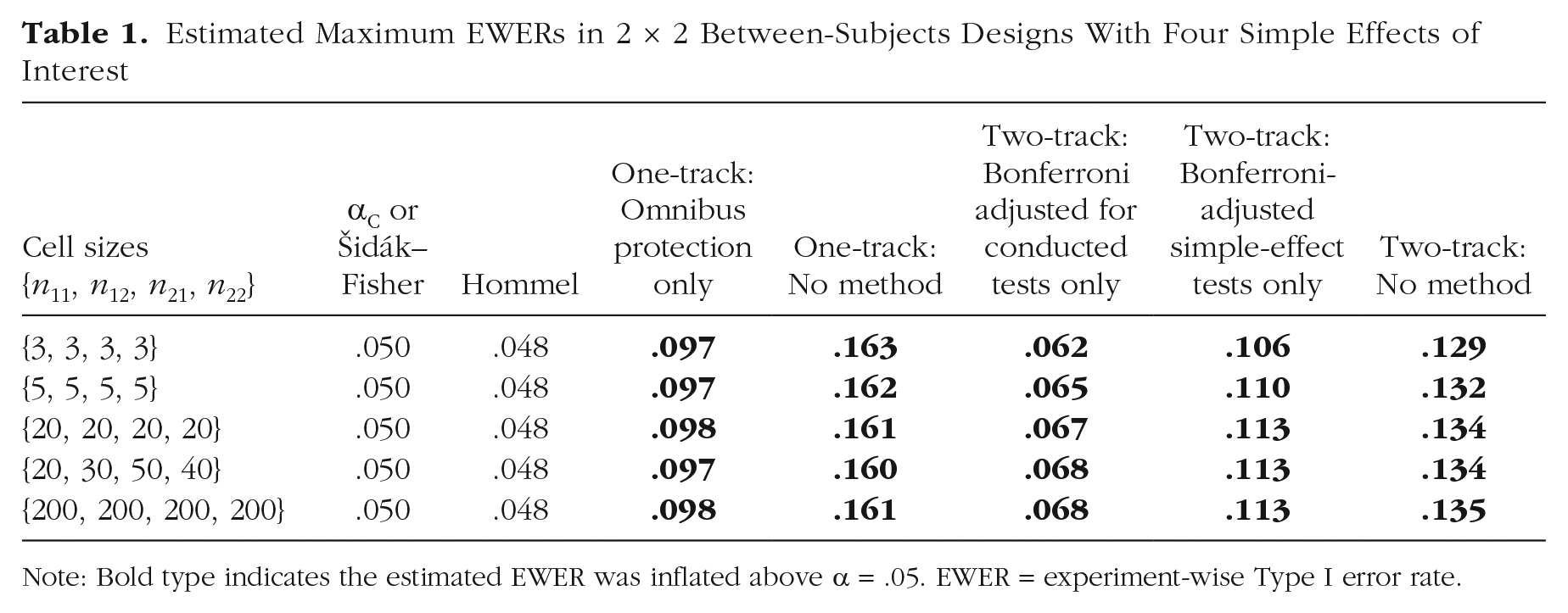
Note: Bold type indicates the estimated EWER was inflated above α = .05. EWER = experiment-wise Type I error rate.

As expected, the α_C and Šidák–Fisher methods (collapsed into a single column in Table 1) controlled the EWER at α. The Hommel procedure controlled the EWER at marginally less than α. The other methods did not control the EWER. Note that with the two-track approach, even Bonferroni adjustment allowed EWER inflation when not all tests that had an a priori potential to be conducted were accounted for in the adjustments. For instance, Bonferroni adjusting only on the simple-effect track inflated the EWER to more than 2α, and Bonferroni adjusting only for the explicitly conducted tests inflated the EWER to more than .06. If a less conservative procedure than Bonferroni were misapplied in the same ways, then the EWER when using these “incomplete” adjustments would be even more inflated.

Six simple effects of interest

Table 2 shows the maximum EWER estimates for between-subjects designs with six simple effects of interest. The α_P, α_C, Hayter–Fisher, and Tukey–Kramer methods (collapsed into a single column in Table 2) controlled the EWER at α. The Hommel procedure controlled the EWER at marginally less than α. Results for the single-step alternatives to Tukey–Kramer were consistent with previous studies (Dunnett, 1980; Kromrey & La Rocca, 1995). Games–Howell was often marginally liberal, Dunnett’s C became increasingly conservative as sample size decreased, Dunnett’s T3 was consi-derably less conservative than Dunnett’s C when sample sizes were small, and Dunnett’s T3 was marginally more conservative than Dunnett’s C when sample sizes were large (although both C and T3 always controlled the EWER). Šidák–Fisher was not examined because the α_P method functions essentially as a sharpened version of Šidák–Fisher in the all-possible-pairs case.

Table 2.

Estimated Maximum EWERs in 2 × 2 Between-Subjects Designs With Six Simple Effects of Interest

Cell sizes{n₁₁, n₁₂, n₂₁, n₂₂}	αP or αC or Tukey–Kramer or Hayter–Fisher	Hommel	Games–Howell	Dunnett’s C	Dunnett’s T3	One-track:Omnibus protection only	One-track:No method	Two-track:Bonferroni-adjusted conducted tests only	Two-track:Bonferroni-adjusted simple only	Two-track:No method
{3, 3, 3, 3}	.050	.047	.049	.013	.039	.124	.208	.058	.102	.129
{5, 5, 5, 5}	.050	.046	.051	.019	.041	.123	.205	.060	.105	.132
{20, 20, 20, 20}	.050	.046	.052	.039	.043	.122	.203	.062	.108	.134
{20, 30, 50, 40}	.050	.046	.051	.043	.042	.122	.201	.062	.108	.134
{200, 200, 200, 200}	.050	.046	.051	.049	.042	.122	.203	.063	.109	.135

Note: Bold type indicates the estimated EWER was inflated above α = .05. EWER = experiment-wise Type I error rate.

The Hayter–Fisher, Tukey–Kramer, Games–Howell, Dunnett’s C, and Dunnett’s T3 procedures were not examined in within-subjects or mixed designs because they are designed for unpaired comparisons. But for the other methods, results in within-subjects and mixed designs were similar to the results in between-subjects designs.

Any-test power

Any-test power is the probability of significance in at least one test of a false null hypothesis. It was estimated as the proportion of iterations in which at least one test of a false null hypothesis was significant. Only methods that controlled the EWER were examined.

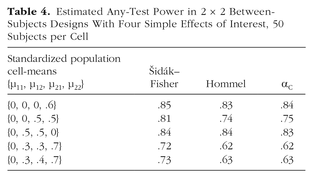
For testing four simple effects, Hommel and α_C had similar any-test power, and Šidák–Fisher tended to have the most any-test power. Tables 3 and 4 show these trends in between-subjects designs with five subjects per cell and 50 subjects per cell, respectively. The same patterns were evident in within-subjects and mixed designs.

Table 3.

Estimated Any-Test Power in 2 × 2 Between-Subjects Designs With Four Simple Effects of Interest, Five Subjects per Cell

Standardized population cell-means {µ₁₁, µ₁₂, µ₂₁, µ₂₂}	Šidák–Fisher	Hommel	α_C
{0, 0, 0, 2}	.77	.71	.71
{0, 0, 2, 2}	.87	.78	.79
{0, 2, 2, 0}	.91	.89	.87
{0, 1, 1, 3}	.87	.78	.78
{0, 1, 2, 3}	.90	.82	.82

Table 4.

Estimated Any-Test Power in 2 × 2 Between-Subjects Designs With Four Simple Effects of Interest, 50 Subjects per Cell

Standardized population cell-means {µ₁₁, µ₁₂, µ₂₁, µ₂₂}	Šidák–Fisher	Hommel	α_C
{0, 0, 0, .6}	.85	.83	.84
{0, 0, .5, .5}	.81	.74	.75
{0, .5, .5, 0}	.84	.84	.83
{0, .3, .3, .7}	.72	.62	.62
{0, .3, .4, .7}	.73	.63	.63

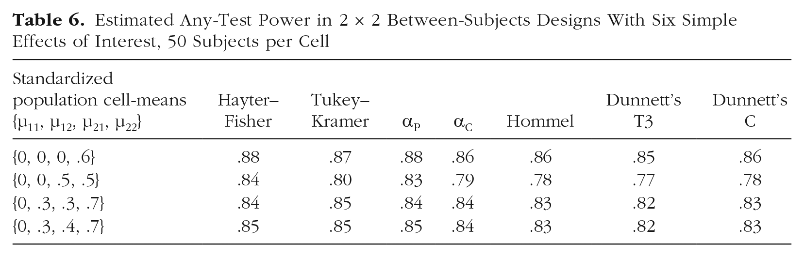
For testing six simple effects in between-subjects designs, Hayter–Fisher often had the most any-test power but was sometimes matched or marginally surpassed by Tukey–Kramer. The α_P tended to perform similarly to Hayter–Fisher and/or Tukey–Kramer. The α_C tended to have marginally more any-test power than Hommel. Hommel tended to have marginally more any-test power than T3. Consistent with Dunnett’s (1980) simulations, T3 was notably more powerful than C when the sample size was small and was marginally less powerful than C when the sample size was large. Tables 5 and 6 show these trends in designs with five subjects per cell and 50 subjects per cell, respectively.

Table 5.

Estimated Any-Test Power in 2 × 2 Between-Subjects Designs With Six Simple Effects of Interest, Five Subjects per Cell

Standardized population cell-means{µ₁₁, µ₁₂, µ₂₁, µ₂₂}	Hayter–Fisher	Tukey–Kramer	α_P	α_C	Hommel	Dunnett’s T3	Dunnett’s C
{0, 0, 0, 2}	.83	.82	.79	.73	.71	.67	.52
{0, 0, 2, 2}	.92	.88	.89	.82	.81	.78	.62
{0, 1, 1, 3}	.96	.97	.95	.91	.90	.88	.77
{0, 1, 2, 3}	.97	.97	.95	.92	.91	.89	.78

Table 6.

Estimated Any-Test Power in 2 × 2 Between-Subjects Designs With Six Simple Effects of Interest, 50 Subjects per Cell

Standardized population cell-means{µ₁₁, µ₁₂, µ₂₁, µ₂₂}	Hayter–Fisher	Tukey–Kramer	α_P	α_C	Hommel	Dunnett’s T3	Dunnett’s C
{0, 0, 0, .6}	.88	.87	.88	.86	.86	.85	.86
{0, 0, .5, .5}	.84	.80	.83	.79	.78	.77	.78
{0, .3, .3, .7}	.84	.85	.84	.84	.83	.82	.83
{0, .3, .4, .7}	.85	.85	.85	.84	.83	.82	.83

Per-test power

Per-test power is the mean probability of significance across all tests of false null hypotheses. It is estimated as the total number of significances in false null hypothesis tests (across all iterations) divided by the total number of false null hypothesis tests (across all iterations). Only methods that controlled the EWER were examined.

Four simple effects of interest

For testing four simple effects, Šidák–Fisher tended to have more per-test power than Hommel, and Hommel tended to have more per-test power than α_C. Tables 7 and 8 show these trends in between-subjects designs with five subjects per cell and 50 subjects per cell, respectively. The same patterns were evident in within-subjects and mixed designs.

Table 7.

Estimated Per-Test Power in 2 × 2 Between-Subjects Designs With Four Simple Effects of Interest, Five Subjects per Cell

Standardized population cell-means {µ₁₁, µ₁₂, µ₂₁, µ₂₂}	Šidák–Fisher	Hommel	α_C
{0, 0, 0, 2}	.64	.56	.54
{0, 0, 2, 2}	.66	.56	.54
{0, 2, 2, 0}	.66	.70	.54
{0, 1, 1, 3}	.42	.40	.33
{0, 1, 2, 3}	.42	.39	.33

Table 8.

Estimated Per-Test Power in 2 × 2 Between-Subjects Designs With Four Simple Effects of Interest, 50 Subjects per Cell

Standardized population cell-means {µ₁₁, µ₁₂, µ₂₁, µ₂₂}	Šidák–Fisher	Hommel	α_C
{0, 0, 0, .6}	.74	.70	.69
{0, 0, .5, .5}	.58	.51	.50
{0, .5, .5, 0}	.58	.60	.50
{0, .3, .3, .7}	.31	.27	.24
{0, .3, .4, .7}	.31	.27	.24

Hommel had slightly more per-test power than Šidák–Fisher only in the special case in which there were four substantial simple effects but no substantial main effects. For example, see the row for population means of {0, 2, 2, 0} in Table 7. In that case, the power of the omnibus test is relatively low (thus weakening Šidák–Fisher), yet there are many opportunities for simple-effect significance (creating a per-test power advantage for Hommel because Hommel lets significance in one test help other tests to be significant). Presumably that is a rare situation because it means that Factor A has a positive effect at one level of Factor B and has an effect that is equally strong in the negative direction at the other level of Factor B.

Six simple effects of interest

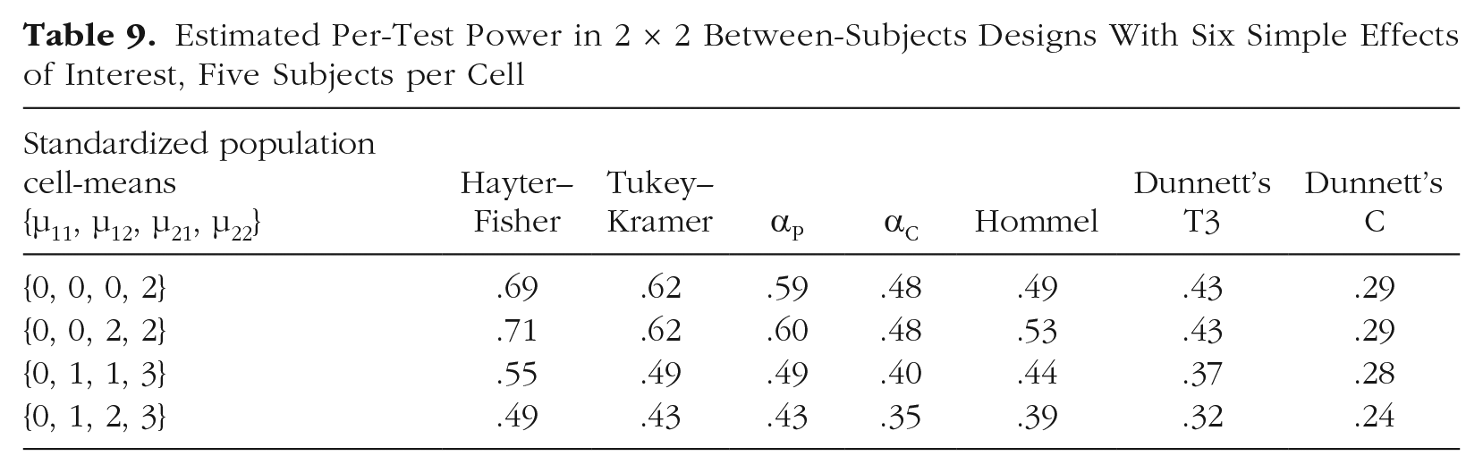
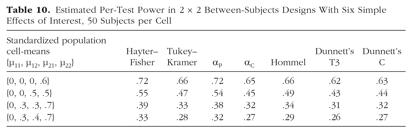
Estimated per-test power in between-subjects designs with six simple effects of interest is shown in Table 9 (for five subjects per cell) and in Table 10 (for 50 subjects per cell). Hayter–Fisher was the clear winner in terms of per-test power (consistent with Kromrey & La Rocca, 1995). The α_P tended to perform similarly to Tukey–Kramer when the sample size was small and to have more per-test power than Tukey–Kramer when the sample size was large. The α_P had more per-test power than Hommel. Hommel tended to have more per-test power than α_C. Power tended to be lowest for Dunnett’s C and T3 procedures. Consistent with Dunnett’s (1980) simulations, T3 was notably more powerful than C when the sample size was small and was marginally less powerful than C when the sample size was large.

Table 9.

Estimated Per-Test Power in 2 × 2 Between-Subjects Designs With Six Simple Effects of Interest, Five Subjects per Cell

Standardized population cell-means {µ₁₁, µ₁₂, µ₂₁, µ₂₂}	Hayter–Fisher	Tukey–Kramer	α_P	α_C	Hommel	Dunnett’s T3	Dunnett’s C
{0, 0, 0, 2}	.69	.62	.59	.48	.49	.43	.29
{0, 0, 2, 2}	.71	.62	.60	.48	.53	.43	.29
{0, 1, 1, 3}	.55	.49	.49	.40	.44	.37	.28
{0, 1, 2, 3}	.49	.43	.43	.35	.39	.32	.24

Table 10.

Estimated Per-Test Power in 2 × 2 Between-Subjects Designs With Six Simple Effects of Interest, 50 Subjects per Cell

Standardized population cell-means {µ₁₁, µ₁₂, µ₂₁, µ₂₂}	Hayter–Fisher	Tukey–Kramer	α_P	α_C	Hommel	Dunnett’s T3	Dunnett’s C
{0, 0, 0, .6}	.72	.66	.72	.65	.66	.62	.63
{0, 0, .5, .5}	.55	.47	.54	.45	.49	.43	.44
{0, .3, .3, .7}	.39	.33	.38	.32	.34	.31	.32
{0, .3, .4, .7}	.33	.28	.32	.27	.29	.26	.27

Consequences of assumption violations

Regarding overall Type I error rates, the consequences of assumption violations are likely trivial compared with the consequences of not adjusting for multiple comparisons. Nonetheless, it is worthwhile to ask how multiple-testing methods perform when assumptions are violated.

Normality

One parametric testing assumption is that the sampling distributions of the mean differences are normal. Because of the central limit theorem, this assumption is typically at least approximately satisfied unless the sample size is very small and/or the population distribution of the variable is extremely nonnormal. Simulations using 10⁷ iterations showed that even when the sample size was small and the population distribution was highly skewed or kurtotic, the viable procedures’ EWER control became only moderately more conservative. For instance, in a between-subjects design with five observations per cell and a χ² population distribution with 5 degrees of freedom (causing extreme positive skewness), the estimated maximum EWER was .044 for the α_C method when four simple effects were of interest. In a between-subjects design with five observations per cell and a Student’s t population distribution with 5 degrees of freedom (causing heavy tails), the estimated maximum EWER was .040 for the α_C method when four simple effects were of interest.

Note that the normality assumption is inherent to the parametric mean comparisons themselves, not to the particular multiple-testing adjustment that is used. Note also that when nonnormality is extreme, it is questionable whether means are even the relevant things to compare. In any case, the impact of nonnormality becomes increasingly trivial as sample size increases.

Equal variance

Between-subjects parametric tests re-quire the assumption of equal population variance. Previous studies have shown by simulation that unequal variances can inflate the EWER when means are equal and variances differ, especially when cell sizes are unequal (e.g., Dunnett, 1980; Sauder & DeMars, 2019). However, although that is a mathematically possible scenario in the world of simulation, it is not very plausible in nature for two populations to have identical means but substantially different variances. Unequal variances are likely when population means are different. But when population means are different, comparing them cannot produce a Type I error. Thus, unequal variances pose a plausible threat to EWER control only when the omnibus error term is used for the pairwise comparisons. In that case, a comparison of two cells with equal means and equal variances can be affected by a third cell with a different mean and a different variance.

Simulations were conducted to demonstrate that when variances differ between cells that have different means, the EWER can become inflated for procedures that use the omnibus error term (i.e., Tukey–Kramer and Hayter–Fisher) but does not become inflated for other procedures. Population means were set to the same values as the corresponding population variances, so the cells with larger population means also had larger population variances, as is often the case in nature. The ratio of larger to smaller variance was set to either 2:1 or 4:1. Cell sizes were set to be either equal, positively correlated with population variance, or negatively correlated with population variance. For each combination of settings, 10⁷ iterations were performed.

Estimated EWERs when population variances were unequal in the six-test case are shown in Table 11 for the 2:1 variance ratio and in Table 12 for the 4:1 variance ratio. Scaling up the cell sizes across the board (e.g., using cell sizes of {50, 50, 100, 100} instead of {5, 5, 10, 10} tended not to hugely affect EWERs, except that the conservatism of Dunnett’s C became less dramatic as sample size increased, as also occurs in the equal variance case). All procedures that controlled the EWER when variances were equal reliably controlled the EWER when variances were unequal except for the two procedures that use the omnibus error term for the pairwise comparisons: Tukey–Kramer and Hayter–Fisher. As shown in Tables 11 and 12, the EWER inflation of those two procedures was largest when cell sizes were negatively correlated with population variances.

Table 11.

Estimated EWERs in 2 × 2 Between-Subjects Designs With Six Simple Effects of Interest, With Unequal Population Variances Equal to the Population Means (2:1 Variance Ratio)

Cell parameters and sizes	Hayter–Fisher	Tukey–Kramer	α_P method	Hommel	α_C method	Dunnett’s T3	Dunnett’s C
µ = σ²: {1, 1, 1, 2} n: {5, 5, 5, 5}	.018	.016	.030	.026	.019	.022	.010
µ = σ²: {1, 1, 1, 2} n: {5, 5, 5, 10}	.012	.009	.029	.027	.019	.022	.010
µ = σ²: {1, 1, 1, 2} n: {10, 10, 10, 5}	.023	.020	.038	.028	.019	.023	.016
µ = σ²: {1, 1, 2, 2} n: {5, 5, 5, 5}	.042	.029	.028	.021	.020	.016	.007
µ = σ²: {1, 1, 2, 2} n: {5, 5, 10, 10}	.032	.020	.028	.021	.020	.016	.009
µ = σ²: {1, 1, 2, 2} n: {10, 10, 5, 5}	.060	.041	.033	.023	.020	.016	.009
µ = σ²: {1, 2, 2, 2} n: {5, 5, 5, 5}	.059	.043	.039	.027	.027	.022	.010
µ = σ²: {1, 2, 2, 2} n: {5, 10, 10, 10}	.051	.035	.042	.027	.027	.023	.016
µ = σ²: {1, 2, 2, 2} n: {10, 5, 5, 5}	.083	.057	.044	.029	.027	.022	.010

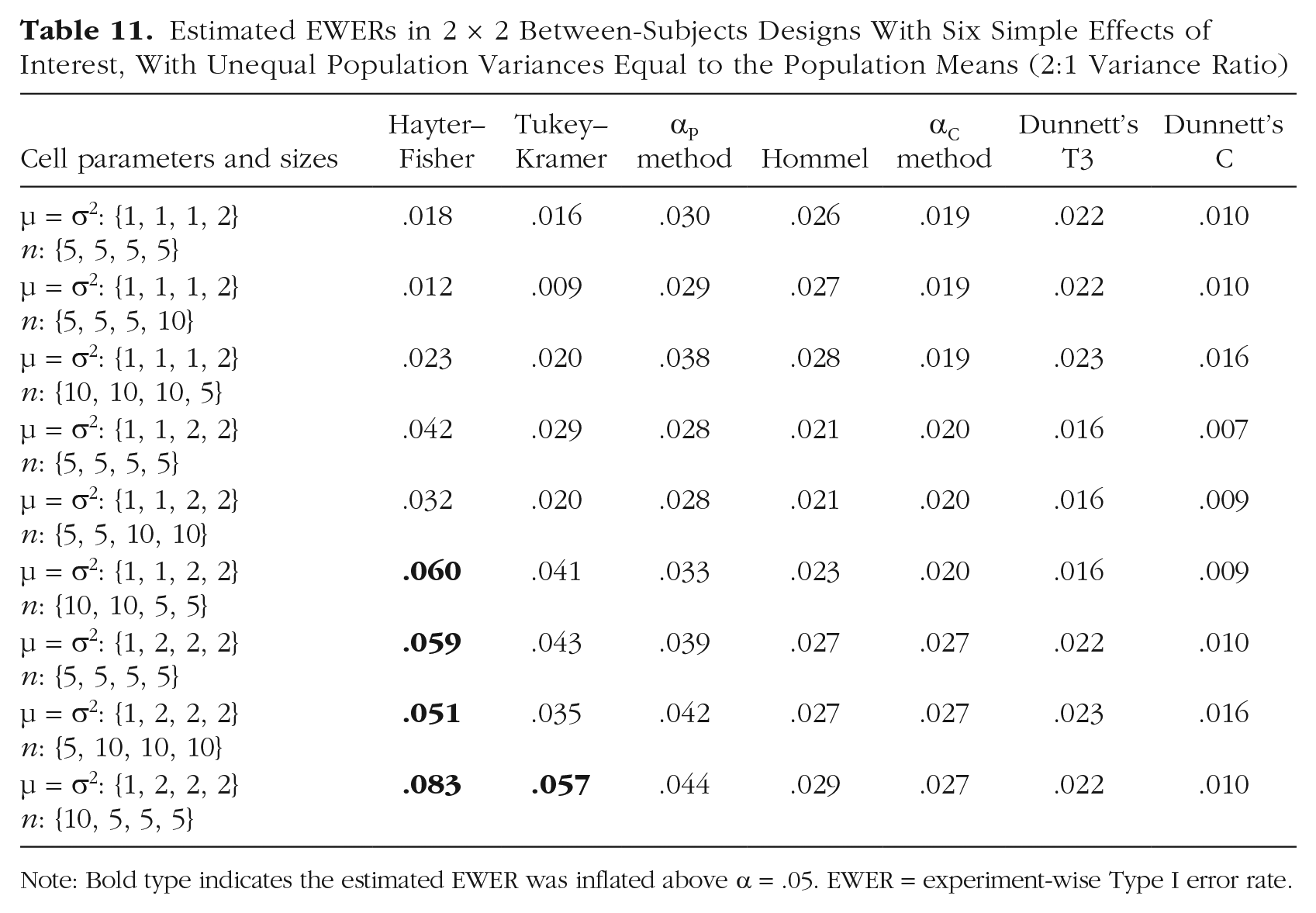
Note: Bold type indicates the estimated EWER was inflated above α = .05. EWER = experiment-wise Type I error rate.

Table 12.

Estimated EWERs in 2 × 2 Between-Subjects Designs With Six Simple Effects of Interest, With Unequal Population Variances Equal to the Population Means (4:1 Variance Ratio)

Cell parameters and sizes	Hayter–Fisher	Tukey–Kramer	α_P method	Hommel	α_C method	Dunnett’s T3	Dunnett’s C
µ = σ²: {1, 1, 1, 4} n: {5, 5, 5, 5}	.010	.007	.046	.036	.027	.022	.010
µ = σ²: {1, 1, 1, 4} n: {5, 5, 5, 10}	.003	.002	.049	.038	.027	.022	.010
µ = σ²: {1, 1, 1, 4} n: {10, 10, 10, 5}	.015	.011	.049	.042	.027	.023	.016
µ = σ²: {1, 1, 4, 4} n: {5, 5, 5, 5}	.065	.043	.036	.033	.020	.016	.007
µ = σ²: {1, 1, 4, 4} n: {5, 5, 10, 10}	.041	.025	.037	.036	.020	.016	.009
µ = σ²: {1, 1, 4, 4} n: {10, 10, 5, 5}	.105	.075	.038	.041	.020	.016	.009
µ = σ²: {1, 4, 4, 4} n: {5, 5, 5, 5}	.085	.054	.049	.036	.027	.022	.010
µ = σ²: {1, 4, 4, 4} n: {5, 10, 10, 10}	.066	.039	.050	.038	.027	.023	.016
µ = σ²: {1, 4, 4, 4} n: {10, 5, 5, 5}	.126	.084	.050	.040	.027	.022	.010

Note: Bold type indicates the estimated EWER was inflated above α = .05. EWER = experiment-wise Type I error rate.

Confidence intervals for effect sizes

A common criticism of p values is that they only facilitate binary decisions about statistical significance and do not provide direct inference regarding effect sizes. If an effect is worth investigating, then presumably the researcher cares not only whether the effect exists but also how large it is. In that regard, confidence intervals are more informative than p values because they not only provide inference about whether the effect is nonzero but also provide a plausible range of effect size estimates. Note that merely looking at the point estimate of an effect size, without considering the confidence interval, is typically not sufficient for making meaningful inferences because estimates vary from sample to sample.

In psychology research, confidence intervals are rarely adjusted for multiple comparisons. However, confidence intervals are subject to the same multiplicity effects that p values are. That is, with every additional unadjusted confidence interval that is computed, the probability that at least one confidence interval will miss the corresponding parameter increases (although such misses may be quantitative and not “all or nothing” errors in the sense that spuriously significant p values are). Thus, when the inferences in a study are based primarily on effect-size estimation—as is often advocated—rather than on null hypothesis testing, adjusting the confidence intervals may be advisable (Bird, 2002, 2004, p. 39; Phillips et al., 2013). In fact, the articles by Dunn (1958, 1961) that are often cited as the canonical references for the Bonferroni procedure actually described adjustment of confidence intervals, not adjustment of null hypothesis tests (see also Šidák, 1967).

It is worth asking which of the examined procedures can be applied to confidence intervals. When a multiple-testing procedure derives all of its Type I error control from comparison-wise α-level adjustments, it can be straightforwardly applied to confidence intervals. Specifically, to achieve an overall confidence level of 1 − α, each individual confidence interval is computed at the 1 − α_adj confidence level, where α_adj is the adjusted comparison-wise α level for the given procedure. Single-step procedures, such as Bonferroni, Šidák, Tukey–Kramer, and the α_C method, can be applied that way. But procedures that do not derive all their Type I error control from adjusted α levels typically cannot be straightforwardly applied to confidence intervals (Shaffer, 1995). Such procedures include Hommel, Hayter–Fisher, Šidák–Fisher, the α_P method, and other multistep procedures that rely on gatekeeping or some other form of conditionality in the testing.

Note that researchers often report standardized effect-size estimates, such as Cohen’s d (the sample mean difference divided by the pooled standard deviation in a between-subjects design). Confidence intervals for standardized effect sizes are easy to compute using the MBESS package in R (Kelley, 2007) and can be adjusted like any other confidence intervals.

Discussion

If PEER control were the accepted standard, then controlling the overall Type I error rate would be relatively simple. The researcher would simply apply the Bonferroni procedure to the tests of interest, thus achieving exact control of the maximum PEER. However, when the goal is to control the FWER/EWER, meaning that multiple co-occurring Type I errors are considered no more costly than a single Type I error, choosing a multiple-testing method becomes more complicated. The most powerful EWER-control procedure is essentially the one that allows the most Type I errors to co-occur. Consequently, numerous EWER-control procedures have been devised to maximize the co-occurrence of Type I errors by exploiting intertest correlation and/or conditional testing structures. The optimal EWER-control procedure in a given situation is the one that provides the most statistical power while still providing robust control of the EWER. With those criteria in mind, in the present study, I evaluated several methods of EWER control in 2 × 2 designs and can now make some simple recommendations.

When four simple effects are of interest in a 2 × 2 design

When four simple effects are of interest (i.e., the two-row simple effects and the two-column simple effects), Šidák–Fisher appears to be the most powerful of the examined methods. But it cannot be applied to confidence intervals. If adjusted confidence intervals are needed (i.e., if inference will be based mainly on effect-size estimation rather than on p values), then the α_C method can be used instead, which in most cases essentially means conducting each test at the .014 level (see the Appendix).

When six simple effects are of interest in a 2 × 2 design

When all six pairwise comparisons are of interest in a between-subjects design, Hayter–Fisher tends to have the most statistical power. But it allows EWER inflation in some plausible unequal-variance situations, as does Tukey–Kramer. Games–Howell does not strictly control the EWER even when assumptions are met. And Dunnett’s C and T3 procedures tend to be less powerful than the other examined methods.

Thus, among the procedures examined here, the competition can be reduced to the α_P and α_C methods. The α_P method tends to be more powerful, but it cannot be applied to confidence intervals. Thus, a reasonable heuristic is to use the α_C method when adjusted confidence intervals are needed and to use the α_P method when adjusted confidence intervals are not needed.

When fewer than four tests are of interest in a 2 × 2 design

In some cases, a researcher might be interested in fewer than four simple effects. For instance, if Factor A were treatment and Factor B were sex, then the researcher might be interested in only the two simple effects of treatment. In that case, omnibus-protected adjustment would not be suitable because there would be only two tests of interest. And the tests would be independent, so there would be no point in trying to exploit intertest correlation. Therefore, if adjusted confidence intervals were not needed, the Hommel procedure would be suitable because it does not rely on intertest correlation or omnibus protection. One could also use the Hochberg (1988) procedure, which is equivalent to Hommel in the two-test case. If adjusted confidence intervals were needed, then the classical Šidák adjustment would be the obvious choice because it is optimized for independent tests.

A variation on the scenario from the preceding paragraph would be a case in which the interaction test was of secondary interest. That is, a researcher’s interest in whether the treatment effect was moderated by sex might be conditional on a treatment effect being detected in both sexes. In that case, one could apply the Hommel/Hochberg procedure to the two simple-effect tests and then—if both simple effects of interest were significant—test the interaction at α. That way, the tests of primary interest would act as gatekeepers, thus controlling the EWER.

Beyond the 2 × 2 design

Simulation-based methods of EWER control, such as the α_C and α_P methods that are recommended here, are straightforwardly adaptable to numerous situations. In fact, the α_C method can be adapted to essentially any design and any family of tests (see also Westfall & Young, 1993). Therefore, given the speed at which modern computers can execute simulations, it is unfortunate that software packages such as IBM SPSS have not made robust simulation-based adjustments more accessible to nonprogrammers. Sauder and DeMars (2019) noted that IBM SPSS offers 18 pairwise-comparison procedures to choose from, some of which are obsolete or unreliable. It would be preferable to offer simulation-based adjustments that are precisely optimized for whatever family of tests is specified by the user.

Conclusions

In the present study, I have recommended some simple, effective methods of EWER control. Researchers who are accustomed to disregarding the EWER may find the idea that they should do otherwise unwelcome. After all, adjusting for multiple comparisons requires investing in larger samples to compensate for reduced statistical power. Nonetheless, those researchers should at least acknowledge that the nominal α level they have been using may substantially understate the overall Type I error rate of the experiment. As the present study’s simulations demonstrate, even a supposedly conservative adjustment, such as the Bonferroni procedure, allows EWER inflation when not all tests that had an a priori potential to be conducted are accounted for in the adjustments.

Regardless of how the family of tests is defined and how Type I error is controlled, it is essential that the researcher state that information a priori—in a verifiable way, such as in a registered study protocol—along with the hypotheses and the complete analysis plan. That does not mean unexpected trends that are discovered in the data should not be investigated. But it does mean that tests of those trends, if performed on the same data that inspired the tests, are essentially descriptive and should not be taken as formal hypothesis tests.

I do not take the view that strict EWER control is mandatory in all cases. Statisticians have long recognized that the proper way to define the family depends on the research situation (e.g., Miller, 1981, pp. 31–35). Any number of approaches may be valid provided that the strength and breadth of the researcher’s claims and inferences are congruent with the approach that is used. There are even cases in which frequentist statistics (i.e., p values and confidence intervals) are not required at all. And in any case, statistical testing should not be the sole basis for inference. One must also consider the quality of the measurements, the plausibility of the proposed mechanism of action, and so on. Statistical analysis is a tool to inform thinking—not a substitute for thinking.

But the fact remains that EWER control is often appropriate, and there is no inherent reason that the 2 × 2 case, or the factorial case in general, should be an exception. Using a less rigorous standard of Type I error control may sometimes be reasonable, but that decision should not be made thoughtlessly and should not be based on arbitrary criteria, such as whether the design is factorial or whether the tests are orthogonal. The analysis should be motivated by the research objectives, not by the design alone.

Supplemental Material

sj-zip-1-amp-10.1177_2515245920985137 – Supplemental material for Experiment-Wise Type I Error Control: A Focus on 2 × 2 Designs

Supplemental material, sj-zip-1-amp-10.1177_2515245920985137 for Experiment-Wise Type I Error Control: A Focus on 2 × 2 Designs by Andrew V. Frane in Advances in Methods and Practices in Psychological Science

Footnotes

Appendix

Transparency

Action Editor: Alexa Tullett

Editor: Daniel J. Simons

Author Contributions

A. V. Frane is the sole author of this article and is responsible for its content.

ORCID iD

Andrew V. Frane

Supplemental Material

Additional supporting information can be found at .

The R programs with filenames that begin with ac2x2 are for obtaining values of α_C and α_P. The R programs with filenames that begin with sim2x2 are for evaluating the power and EWER-control of the methods examined in this article. The pdf file provides details about the programs.

References

Albert

Rizzo

(2012). R by example. Springer.

Barnette

J. J.

McLean

J. E.

(2005). Type I error of four pairwise mean comparison procedures conducted as protected and unprotected tests. Journal of Modern Applied Statistical Methods, 4(2), 446–459. https://doi.org/10.22237/jmasm/1130803740

Benjamini

Hochberg

(1995). Controlling the false discovery rate: A practical and powerful approach to multiple testing. Journal of the Royal Statistical Society, Series B (Methodological), 57(1), 289–300. https://doi.org/10.1111/j.2517-6161.1995.tb02031.x

Bethea

R. M.

Duran

B. S.

Boullion

T. L.

(1995). Statistical methods for engineers and scientists (3rd ed.). CRC.

Bibby

(2012). Simple main effects. In Salkind

N. J.

(Ed.), Encyclopedia of research design (pp. 1376–1380). SAGE.

Bird

K. D.

(2002). Confidence intervals for effect sizes in analysis of variance. Educational and Psychological Measurement, 62(2), 197–226. https://doi.org/10.1177/0013164402062002001

Bird

K. D.

(2004). Analysis of variance via confidence intervals. SAGE.

Bobko

(1986). A solution to some dilemmas when testing hypotheses about ordinal interactions. Journal of Applied Psychology, 71(2), 323–326. https://doi.org/10.1037/0021-9010.71.2.323

Brown

S. R.

Melamed

L. E.

(1990). Experimental design and analysis. SAGE.

10.

Cardinal

R. N.

Aitken

M. R.

(2006). ANOVA for the behavioural sciences researcher. Erlbaum.

11.

Cohen

West

S. G.

Aiken

L. S.

(2003). Applied multiple regression/correlation analysis for the behavioral sciences (3rd ed.). Erlbaum.

12.

Cramer

A. O. J.

van Ravenzwaaij

Matzke

Steingroever

Wetzels

Grasman

R. P. P. P.

Waldorp

L. J.

Wagenmakers

E.-J.

(2016). Hidden multiplicity in exploratory multiway ANOVA: Prevalence and remedies. Psychonomic Bulletin & Review, 23, 640–647. https://doi.org/10.3758/s13423-015-0913-5

13.

Devore

J. L.

(1987). Probability and statistics for engineering and the sciences (2nd ed.). Brooks/Cole.

14.

Dunn

O. J.

(1958). Estimation of the means of dependent variables. The Annals of Mathematical Statistics, 29(4), 1095–1111. https://www.jstor.org/stable/2236948

15.

Dunn

O. J.

(1961). Multiple comparisons among means. Journal of the American Statistical Association, 56(293), 52–64. https://doi.org/10.1080/01621459.1961.090

16.

Dunnett

C. W.

(1955). A multiple comparison procedure for comparing several treatments with a control. Journal of the American Statistical Association, 50(272), 1096–1121. https://doi.org/1080/01621459.1955.10501294

17.

Dunnett

C. W.

(1980). Pairwise multiple comparisons in the unequal variance case. Journal of the American Statistical Association, 75(372), 796–800. https://doi.org/10.1080/01621459.1980.10477552

18.

Edwards

Berry

J. T.

(1987). The efficiency of simulation-based multiple comparisons. Biometrics, 43(4), 913–928.

19.

Fisher

R. A.

(1935). The design of experiments. Oliver & Boyd.

20.

Frane

A. V.

(2015a). Are per-family Type I error rates relevant in social and behavioral science? Journal of Modern Applied Statistical Methods, 14(1), 12–23. https://doi.org/10.22237/jmasm/1430453040

21.

Frane

A. V.

(2015b). Planned hypothesis tests are not necessarily exempt from multiplicity adjustment. Journal of Research Practice, 11(1), Article P2. http://jrp.icaap.org/index.php/jrp/article/view/514/417

22.

Games

P. A.

Howell

J. F.

(1976). Pairwise multiple comparison procedures with unequal n’s and/or variances: A Monte Carlo study. Journal of Educational Statistics, 1(2), 113–125. https://doi.org/10.3102/10769986001002113

23.

Girden

E. R.

(1992). ANOVA: Repeated measures. SAGE.

24.

Gonzalez

(2009). Data analysis for experimental design. Guilford.

25.

Hancock

G. R.

Klockars

A. J.

(1996). The quest for α: Developments in multiple comparison procedures in the quarter century since Games (1971). Review of Educational Research, 66(3), 269–306. https://doi.org/10.3102/00346543066003269

26.

Hays

W. L.

(1988). Statistics (4th ed.). Holt, Rinehart and Winston.

27.

Hayter

A. J.

(1986). The maximum familywise error rate of Fisher’s least significant difference test. Journal of the American Statistical Association, 81(396), 1000–1004. https://doi.org/10.1080/01621459.1986.10478364

28.

Heiberger

R. M.

Holland

(2004). Statistical analysis and data display: An intermediate course with examples in S-Plus, R, and SAS. Springer.

29.

Hochberg

(1988). A sharper Bonferroni procedure for multiple tests of significance. Biometrika, 75(4), 800–802. https://doi.org/10.1093/biomet/75.4.800

30.

Hochberg

Tamhane

A. C.

(1987). Multiple comparison procedures. John Wiley & Sons.

31.

Holm

(1979). A simple sequentially rejective multiple test procedure. Scandinavian Journal of Statistics, 6(2), 65–70.

32.

Hommel

(1988). A stagewise rejective multiple test procedure based on a modified Bonferroni test. Biometrika, 75(2), 383–386. https://doi.org/10.1093/biomet/75.2.383

33.

Howell

D. C.

(2013). Statistical methods for psychology (8th ed.). Wadsworth.

34.

Hsu

J. C.

Nelson

(1998). Multiple comparisons in the general linear model. Journal of Computational and Graphical Statistics, 7(1), 23–41. https://doi.org/10.1080/10618600.1998.10474759

35.

Huberty

C. L.

Morris

J. D.

(1988). A single contrast test procedure. Educational and Psychological Measurement, 48(3), 567–578. https://doi.org/10.1177/0013164488483001

36.

Kelley

(2007). Confidence intervals for standardized effect sizes: Theory, application, and implementation. Journal of Statistical Software, 20(8). https://doi.org/10.18637/jss.v020.i08

37.

Kirk

R. E.

(2013). Experimental design: Procedures for the behavioral sciences (4th ed.). SAGE.

38.

Klockars

A. J.

Hancock

G. R.

McAweeney

M. J.

(1995). Power of unweighted and weighted versions of simultaneous and sequential multiple-comparison procedures. Psychological Bulletin, 118(2), 300–307. https://doi.org/10.1037/0033-2909.118.2.300

39.

Kramer

C. Y.

(1956). Extension of multiple range tests to group means with unequal numbers of replications. Biometrics, 12(3), 307–310. https://doi.org/10.2307/3001469

40.

Kromrey

J. D.

Dickinson

W. B.

(1995). The use of an overall F test to control Type I error rates in factorial analyses of variance: Limitations and better strategies. The Journal of Applied Behavioral Science, 31(1), 51–64. https://doi.org/10.1177/0021886395311006

41.

Kromrey

J. D.

La Rocca

M. A.

(1995). Power and Type I error rates of new pairwise comparison procedures under heterogeneous variances. The Journal of Experimental Education, 63(4), 343–362. https://doi.org/10.1080/00220973.1995.9943469

42.

Lawrence

(2019). Familywise and per-family error rates of multiple comparison procedures. Statistics in Medicine, 38(19), 3586–3598. https://doi.org/10.1002/sim.8190

43.

Levin

J. R.

Serlin

R. C.

Seaman

M. A.

(1994). A controlled, powerful multiple comparisons strategy for several situations. Psychological Bulletin, 115(1), 153–159. https://doi.org/10.1037/0033-2909.115.1.153

44.

Luck

S. J.

Gaspelin

(2017). How to get statistically significant effects in any ERP experiment (and why you shouldn’t). Psychophysiology, 54(1), 146–157. https://doi.org/10.1111/psyp.12639

45.

Ludbrook

(1991). On making multiple comparisons in clinical and experimental pharmacology and physiology. Clinical and Experimental Pharmacology and Physiology, 18, 379–392. https://doi.org/10.1111//j.1440-1681.1991.tb01468.x

46.

Maxwell

S. E.

Delaney

H. D.

Kelley

(2018). Designing experiments and analyzing data: A model comparison perspective (3rd ed.). Routledge.

47.

Miller

R. G.

Jr. (1981). Simultaneous statistical inference (2nd ed.). Springer-Verlag.

48.

Nestor

P. G.

Schutt

R. K.

(2012). Research methods in psychology: Investigating human behavior. SAGE.

49.

Phillips

Fletcher

Atkinson

Channon

Douiri

Jaki

Maca

Morgan

Roger

J. H.

Terrill

(2013). Multiplicity: Discussion points from the Statisticians in the Pharmaceutical Industry multiplicity expert group. Pharmaceutical Statistics, 12(5), 255–259. https://doi.org/10.1002/pst.1584

50.

Ramsey

P. H.

Barrera

Hachimine-Semprebom

Liu

C.-C.

(2011). Pairwise comparisons of means under realistic nonnormality, unequal variances, outliers and equal sample sizes. Journal of Statistical Computation and Simulation, 81(2), 125–135. https://doi.org/10.1080/00949650903219935

51.

Rosnow

R. L.

Rosenthal

(1989). Definition and interpretation of interaction effects. Psychological Bulletin, 105(1), 143–146. https://doi.org/10.1037/0033-2909.105.1.143

52.

Ryan

T. A.

(1962). The experiment as the unit for computing rates of error. Psychological Bulletin, 59(4), 301–305. https://doi.org/10.1037/h0040562

53.

Sauder

D. C.

DeMars

C. E.

(2019). An updated recommendation for multiple comparisons. Advances in Methods and Practices in Psychological Science, 2(1), 26–44. https://doi.org/10.1177/2515245918808784

54.

Shaffer

J. P.

(1979). Comparison of means: An F test followed by a modified multiple range procedure. Journal of Educational and Behavioral Statistics, 4(1), 14–23. https://doi.org/10.3102/10769986004001014

55.

Shaffer

J. P.

(1986). Modified sequentially rejective multiple test procedures. Journal of the American Statistical Association, 81(395), 826–831. https://doi.org/10.1080/01621459.1986.10478341

56.

Shaffer

J. P.

(1991). Probability of directional errors with disordinal (qualitative) interaction. Psychometrika, 56(1), 29–38.

57.

Shaffer

J. P.

(1995). Multiple hypothesis testing. Annual Review of Psychology, 46, 561–584. https://doi.org/10.1146/annurev.ps.46.020195.003021

58.

Sheskin

D. J.

(2007). Handbook of parametric and nonparametric statistical procedures (4th ed.). Chapman & Hall.

59.

Šidák

(1967). Rectangular confidence regions for the means of multivariate normal distributions. Journal of the American Statistical Association, 62(318), 626–633. https://doi.org/10.1080/01621459.1967.10482935

60.

Small

D. S.

Volpp

K. G.

Rosenbaum

P. R.

(2011). Structured testing of 2×2 factorial effects: An analytic plan requiring fewer observations. The American Statistician, 65(1), 11–15. https://doi.org/10.1198/tast.2011.10130

61.

Spjøtvoll

(1972). On the optimality of some multiple comparison procedures. The Annals of Mathematical Statistics, 43(2), 398–411. https://doi.org/10.1214/aoms/1177692621

62.

Steinfatt

T. M.

(1979). The alpha percentage and experimentwise error rates in communication research. Human Communication Research, 5(4), 366–374. https://doi.org/10.1111/j.1468-2958.1979.tb00650.x

63.

Tamhane

A. C.

(1979). A comparison of procedures for multiple comparisons of means with unequal variances. Journal of the American Statistical Association, 74(366a), 471–480. https://doi.org/10.1080/01621459.1979.10482541

64.

Tamhane

A. C.

(2009). Statistical analysis of designed experiments: Theory and applications. John Wiley & Sons.

65.

Toothaker

L. E.

(1993). Multiple comparison procedures. SAGE.

66.

Tukey

J. W.

(1953). The problem of multiple comparisons. In Braun

H. I.

(Ed.), The collected works of John W. Tukey, Vol. VIII. Multiple comparisons: 1948–1983 (pp. 1–300). Chapman & Hall.

67.

Weber

D. C.

Skillings

J. H.

(2000). A first course in the design of experiments. CRC.

68.

Westfall

P. H.

Tobias

R. D.

Wolfinger

R. D.

(2011). Multiple comparisons and multiple tests using SAS (2nd ed.). SAS Institute.

69.

Westfall

P. H.

Young

S. S.

(1993). Resampling-based multiple testing. John Wiley & Sons.

70.

Williams

J. D.

(1973). Note on familywise error rates. Psychological Reports, 32, 1221–1222. https://doi.org/10.2466/pr0.1973.32.3c.1221

Supplementary Material

Please find the following supplemental material available below.

For Open Access articles published under a Creative Commons License, all supplemental material carries the same license as the article it is associated with.

For non-Open Access articles published, all supplemental material carries a non-exclusive license, and permission requests for re-use of supplemental material or any part of supplemental material shall be sent directly to the copyright owner as specified in the copyright notice associated with the article.

0.12 MB

0.00 MB

Experiment-Wise Type I Error Control: A Focus on 2 × 2 Designs

Abstract

Keywords

The 2 × 2 Design

The Overall Type I Error Rate in 2 × 2 Designs

Conventional Approaches to Type I Error Control in Factorial Designs

No adjustment

Omnibus protection

Leaving the main-effect tests unadjusted

Disregarding the simple effects

Viable Methods of EWER Control in Factorial Designs

Simulation-based adjustment (the αC method)

Hommel procedure

Single-step all-possible-pairs methods

Other commonly available methods

Protected adjustment

When four simple effects are of interest

When six simple effects are of interest

Evaluation of the Methods

Maximum EWER

Four simple effects of interest

Six simple effects of interest

Any-test power

Per-test power

Four simple effects of interest

Six simple effects of interest

Consequences of assumption violations

Normality

Equal variance

Confidence intervals for effect sizes

Discussion

When four simple effects are of interest in a 2 × 2 design

When six simple effects are of interest in a 2 × 2 design

When fewer than four tests are of interest in a 2 × 2 design

Beyond the 2 × 2 design

Conclusions

Supplemental Material

sj-zip-1-amp-10.1177_2515245920985137 – Supplemental material for Experiment-Wise Type I Error Control: A Focus on 2 × 2 Designs

Footnotes

Appendix

Transparency

ORCID iD

Supplemental Material

References

Supplementary Material

Simulation-based adjustment (the α_C method)