Analyzing Individual Differences in Intervention-Related Changes

Abstract

Intervention studies can be expensive and time-consuming, which is why it is important to extract as much knowledge as possible. We discuss benefits and limitations of analyzing individual differences in intervention studies in addition to traditional analyses of average group effects. First, we present a short introduction to latent change modeling and measurement invariance in the context of intervention studies. Then, we give an overview on options for analyzing individual differences in intervention-related changes with a focus on how substantive information can be distinguished from methodological artifacts (e.g., regression to the mean). The main topics are benefits and limitations of predicting changes with baseline data and of analyzing correlated change. Both approaches can offer descriptive correlational information about individuals in interventions, which can inform future variations of experimental conditions. Applications increasingly emerge in the literature—from clinical, developmental, and educational psychology to occupational psychology—and demonstrate their potential across all of psychology.

Individual experiences and behavior are the core of psychological science. Psychological theories often center around mechanisms, antecedents, and consequences of individual functioning. Psychological assessment commonly acknowledges individuals as one dimension of psychological observations (together with time points and variables; Cattell & Nesselroade, 1988). Applied psychology aims to understand and support individuals in diverse contexts such as school, occupation, and retirement. From a theoretical, methodological, and applied perspective, interventions are an informative study design. However, especially the information about individuals and individual functioning is not always fully explored by traditional approaches of analyzing intervention studies. Traditionally, the main question is whether an intervention leads to significant average improvements compared with one or more control conditions. This is a crucial test of the overall effectiveness of an intervention and—in the case of a randomized controlled trial with an appropriate control condition—even allows for causal inferences (Shadish et al., 2002). However, such group differences may say little about the impact of the intervention on the individuals being studied (cf. McArdle & Prindle, 2008). For example, there can be significant average group effects of an intervention on two variables (compared with the control condition), but both effects are based on different individuals. Furthermore, there can be individual effects without group effects (McArdle & Prindle, 2008). Thus, we discuss benefits and challenges of analyzing individual differences in intervention studies in addition to average group effects. The methods for analyzing individual differences discussed here cannot replace analyses of group effects and do not allow any causal inferences. Instead, they can provide correlational and descriptive information about individuals and interventions, which can, for example, enhance the interpretation of interventions and, in the long-term, the implementation of interventions (e.g., adapting interventions to individual characteristics). We use latent change models as a framework for analyzing individual differences in interventions because they are especially suitable for typical applications with two or three groups (e.g., intervention, active control, passive control) and two or three time points (pretest, posttest, follow-up). Thus, we begin with a short introduction to latent change models and important concepts in this context (e.g., measurement invariance) before we address our main issue of individual differences in intervention-related changes.

Latent Change Modeling

Latent change models (for an overview, see McArdle, 2009) are also called latent change score models, latent difference (score) models, and latent true change models. Latent change models with measurement models have been referred to as second-order latent change (score) models (e.g., Ferrer et al., 2008), but this distinction (first-order/second-order, i.e., without/with measurement models) is not consistently applied across the literature. In the present article, we address second-order latent change models, which are particularly eligible for analyzing individual differences in interventions. They can be estimated as multiple-group latent change models and allow researchers to analyze latent constructs and latent changes in constructs across both time points and groups (Fig. 1). They are based on the same statistical assumptions as all structural equation models with latent variables (for details, see Kline, 2012), which are generally more flexible in testing and accounting for these assumptions than other statistical techniques (e.g., analysis of variance). Especially relevant for using multiple-group latent change models in the context of interventions is that (a) measurement invariance across time points and groups can be tested and evaluated (content of a later section), (b) nonnormality in the distribution of empirical data can be addressed by using robust estimators (for details, see Lei & Wu, 2012), (c) an appropriate measurement model can distinguish true score and error variance of a construct by differentiating common and unique sources of variance in indicators of this construct, and (d) if a latent factor is considered free of measurement error at two time points (e.g., preintervention and postintervention), then the latent change between both is also considered free of measurement error (cf. McArdle & Prindle, 2008). Thus, analyzing latent change scores is preferable to analyzing observed difference scores (for a detailed review of the latter, see Trafimow, 2015). However, if the estimated measurement model differs considerably from the true relation between the construct and its indicators, then the latent factor will be a poor proxy for the construct (cf. Rhemtulla et al., 2020). Choosing a measurement model is therefore a crucial step in latent change modeling. Most importantly, indicators are considered to be mutually uncorrelated after controlling for their common factor (i.e., local independence), and the construct is equivalent to whatever is common among its indicators (and not a combination of its indicators; Rhemtulla et al., 2020). If both aspects are considered during the selection of theoretically meaningful indicators, latent change models can adequately control for measurement error. Most latent variable models in psychology are reflective models, which means that the responses on the indicators are considered to vary as a function of the latent variable, or in other words, “variation in the latent variable precedes variation in the indicators” (cf. Borsboom et al., 2003, p. 208). Intervention research can use these directed assumptions in latent variables to test theories on the structure and functioning of the psychological construct of interest (for details, see Protzko, 2017), which is another advantage of analyzing latent change scores. Finally, as in all structural equation models with latent variables, one should evaluate how well the hypothesized model fits the observed data, usually with a χ² test statistic and descriptive fit indices (for details, see West et al., 2012).

Fig. 1.

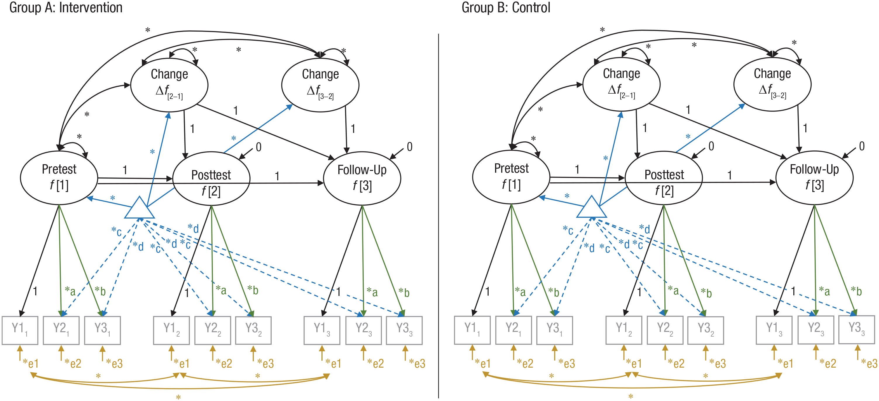
Multiple-group latent change model with strict measurement invariance across group (intervention, control) and time (pretest, posttest, follow-up). Squares represent observed variables, circles represent latent variables, asterisks represent free parameters, and the triangle represents mean and intercept information (dashed lines are free intercepts). Parameters with the same name are constrained to be equal (are estimated on the same unstandardized value). For model identification, the first factor loading of each latent variable is fixed to 1. Correlated error terms of the same indicator across time are allowed (exemplary shown for e1). Failing to specify covariates between error terms of the same indicator across time (or method factors capturing these covariances) can lead to biased estimations of structural relations and decreased model fit (e.g., Pitts et al., 1996). Factor loadings (a, b), intercepts (c, d), and error terms (e1, e2, e3) are constrained to be equal across groups and time. Y1–Y3 = observed indicator variables; Δ = difference.

Latent change models use a set of fixed coefficients (fixed to 1) to define a later measurement occasion (e.g., Fig. 1: f[2]) as the sum of an earlier occasion (f[1]) and the difference (Δf_[2–1]) between both: f[2] = f[1] + Δf_[2–1], or Δf_[2–1] = f[2] – f[1] (McArdle, 2009). Thus, the change between two time points is represented as a latent variable with a mean (i.e., average change), a variance (i.e., individual differences in change), and a covariation of the change with the initial factor f[1] and, if applicable, other factors in the model. In other words, the model allows one to estimate not only latent means and latent intraindividual mean changes (e.g., between preintervention and postintervention) but also interindividual differences in both. In the case of, for example, a follow-up assessment, an additional latent change score can be modeled to capture the change between postintervention and follow-up (e.g., Fig. 1: Δf_[3–2]). Because the direction of change between the measurement occasions is independent, the latent score can increase over one time period (e.g., Δf_[2–1]) and be stable or even decrease over the next (e.g., Δf_[3–2]). This is especially suitable for interventions, in which the greatest change in the outcome often occurs early (e.g., because of the law of practice, Heathcote et al., 2000; see e.g., Gross et al., 2013) and may not remain stable until follow-up. Furthermore, both latent change variables can have differential predictors (cf. Goldsmith et al., 2018), which is crucial because the factors contributing to intervention-related gains may not be same as the factors contributing to maintenance after intervention.

Note that when specified as a multiple-group model, one can test for any intervention-related differences by comparing the fit of the model when a parameter is either constrained to be equal or free to vary across the intervention and control groups (McArdle & Prindle, 2008). For example, one can test for average group effects by constraining the means of the latent change between the preassessment and postassessment of an outcome variable to be equal in the intervention group and an adequate control group. If such a constraint significantly decreases the model fit, then the groups significantly differ in the latent change between the preassessment and postassessment.

Latent change models and latent growth curve models belong to the same family of structural equation models (e.g., Ghisletta & McArdle, 2012) and are even statistically equivalent in special cases (with specific parameter restrictions). Latent change models are typically parameterized to predict changes between time points (e.g., Δf_[2–1] = f[2] – f[1]), whereas latent growth curve models are typically parameterized to predict growth (e.g., f[2] = f[1] + Δf_[2–1]) in the value of a variable (cf. Bainter & Howard, 2016). However, it is obvious that in this example, both are equivalent reparameterizations of each other. In addition, in more complex situations, change is considered an accumulation of the first differences among latent variables in latent change models, and latent growth models can typically be reconceptualized in terms of first differences (e.g., McArdle & Grimm, 2010). Yet in most applications, they differ considerably (e.g., model specifications, underlying function of change, usage of defaults) and for this reason are suitable to test both overlapping and different research questions (e.g., for an overview, see Bainter & Howard, 2016, Table 1). More detailed comparisons of both approaches are available in the literature (e.g., Ferrer et al., 2008; McArdle, 2009; McArdle & Grimm, 2010), as are more detailed descriptions of latent change models with code examples for various software packages (Ghisletta & McArdle, 2012: sem, lavaan, and OpenMx packages in R; Kievit et al., 2018: Lavaan package in R and Ωnyx software; Klopack & Wickrama, 2020: Mplus software). In the following, we focus on selected issues that are particularly relevant in the context of interventions.

Practical Issues and Challenges in Latent Change Modeling

Differences between findings based on latent variables compared with observed variables

There are many reasons to use latent variable models wherever possible (for details, see Borsboom, 2008) from both theoretical and practical perspectives (e.g., that many psychological constructs are inherently latent or that they provide a more appropriate consideration of measurement error). However, it is possible that an intervention has significant average group effects on some indicators of a latent variable but not on the latent variable itself (i.e., the common variance does not capture the effect; e.g., Estrada et al., 2015) or that an effect is significant on a latent level but not present in all indicators (e.g., Schmiedek et al., 2010). This is not surprising because of many reasons; for example, indicators differ in their reliability, their sensitivity to change, and their relation to the construct (e.g., they can measure different facets or subprocesses that can be differentially affected by an intervention). A solution to this issue is to report the average group findings on both a latent level and an observed level (e.g., Fig. 3 in Schmiedek et al., 2010).

Choice and impact of covariates

Including covariates, for example time-invariant covariates such as high school grade point average or time-varying covariates such as health status, can reduce omitted variable bias and enhance inferences in intervention research (e.g., for details, see Pearl et al., 2016, p. 70). However, in all statistical procedures, the choice of covariates can strongly affect the interpretation of the findings (e.g., Silberzahn et al., 2018) and, in extreme cases, even lead to wrong conclusions (e.g., in the case of colliders ¹ ; for details, see Pearl et al., 2016, p. 40). In structural equation modeling, the fit of the hypothesized model to the observed data is evaluated (for details, see West et al., 2012), and the covariates as well as their relations to all other variables are a part of this model. Thus, all covariates need to be selected carefully with a consideration of the overall model complexity (for examples of latent change modeling with covariates, see McArdle & Prindle, 2008; Zelinski et al., 2014). All covariates represented as latent variables should be analyzed separately before they are included in latent change models for intervention outcomes. For example, one should evaluate the measurement model of a covariate and test measurement invariance across groups and, if applicable, time (for time-varying covariates assessed at multiple time points). The findings with and without covariates are informative, and both should be reported (e.g., one can be included in an online appendix).

Missing data

Missing data is a particularly relevant topic in intervention studies because study dropout in longitudinal designs is common. Rubin (1976) differentiated three types of missing data: (a) missing completely at random (MCAR); (b) missing at random (MAR), in which the probabilities of missingness depend on observed data but not on missing data (both are considered ignorable nonresponse); and (c) missing not at random (MNAR), in which the probabilities of missingness depend on missing data (nonignorable nonresponse). Standard full information maximum likelihood estimation requires missing data to be MCAR or MAR and can result in considerable parameter estimate biases if the data are MNAR (for details, see Graham, 2003). Theoretical and practical considerations about one’s data (e.g., known information about the population, practical observations during data collection) can be accompanied by test statistics for MCAR (e.g., Jamshidian & Jalal, 2010; Little, 1988). For example, Little’s (1988) χ² test is a global test statistic using all available data and thus avoids multiple-comparison problems (for an application in an intervention study, see Maass et al., 2015). If MNAR is likely, for example because of selective noncompliance, or if the observed variables associated with missingness in MAR are not included in the inferential model or models, adding auxiliary variables to the analysis can substantially reduce or even eliminate parameter estimate biases (Graham, 2003). Auxiliary variables are observed variables that are predictive of the variables containing missingness and/or the causes of missingness. The former type is quite common and thus easy to implement (for an application in an intervention study, see Gellert et al., 2014). This is one major reason why analyzing predictors of pretest, change, posttest, and (if available) follow-up data is informative and can improve the estimation of the inferential model or models (e.g., testing treatment effects). More details on missing data diagnostics and treatment (e.g., Enders, 2010; Lang & Little, 2018) as well as on reducing the likelihood of missing data in the first place (Little et al., 2012) can be found in the literature.

Sample size and statistical power

In general, the literature clearly suggests an inverse relation between sample size on the one hand and the extent of estimation bias (parameter and standard error estimates) as well as the frequency of improper solutions (e.g., negative variance estimates) on the other hand (e.g., Chen et al., 2001; Hoogland & Boomsma, 1998). Furthermore, higher values of the ratio of observations to estimated parameters (N:q) are preferred because they are associated with a higher accuracy of model-fit evaluation (Jackson, 2003). However, common sample size suggestions and easy rules of thumb (e.g., “at least 200 observations,” “at least 10 observations per estimated parameter”) can be misleading because they are typically not model-specific (e.g., Wolf et al., 2013). Results of robustness studies are valid only for the simulated conditions unless a consistent picture emerges in the field. For example, a meta-analysis of robustness studies included suggestions for a variety of models and data distributions (Hoogland & Boomsma, 1998, Table 4). Still, such suggestions cannot replace a power analysis in the context of a specific research question. Methods of power estimation can be distinguished in model-based approaches, such as Monte Carlo simulation (e.g., L. K. Muthén & Muthén, 2002) and the parametric misspecification approach (Satorra & Saris, 1985), and approaches according to model-fit indices, such as the overall model-fit approach (MacCallum et al., 1996) and its extensions (e.g., Kim, 2005). Choosing a suitable approach for an individual research question depends mostly on three factors: (a) a priori or a posteriori power analysis (e.g., Wagenmakers et al., 2015), (b) confirmatory or exploratory research questions (e.g., Lee et al., 2012), and (c) focus on multiple model parameters or one or two key parameters (e.g., Lee et al., 2012).

For example, in an a priori/confirmatory/focus on multiple model parameters case (e.g., a preregistered trial with multiple confirmatory hypotheses), Monte Carlo simulations are the state of the art for power estimations (for a general introduction, see L. K. Muthén & Muthén, 2002; for details on latent change models, see Zhang & Liu, 2019). In Monte Carlo simulations, one specifies a hypothesized population value for each parameter of a model (according to previous research and theory) and then generates random samples/replications of model estimations, which provide information about all parameters and overall model fit (power and estimation precision). To enhance their accessibility and applicability, user-friendly online interfaces and packages have been developed recently (e.g., Brandmaier et al., 2015; Zhang & Liu, 2019). ² However, although they are particularly designed to provide an easy access to estimate the power of latent change models, the model needed for a specific research question (e.g., with a specific pattern of covariates) might not be available in these tools. Kievit and colleagues (2018) provided a commented R script for power estimation in latent change models that can be individually adapted to the given design and research question (freely available at https://osf.io/8xhmt/, as of August 1, 2020).

In an a priori/confirmatory/focus on one or two key model parameters case (e.g., replicating a known effect), the parametric misspecification approach (Satorra & Saris, 1985) could be helpful (for details, see Lee et al., 2012; for an illustration for interventions, see B. O. Muthén & Curran, 1997). Here, one specifies null and alternative models that differ only in parameter restrictions (i.e., are nested models). Because the approximated effect size is a direct function of these parameter restrictions, this approach provides information “only” about specific parameters (e.g., the power for testing a mean difference or correlation).

In an a priori/exploratory/focus on multiple model parameters case (e.g., testing a novel treatment), model-fit approaches (e.g., Kim, 2005; MacCallum et al., 1996) could be helpful (for details, see Lee et al., 2012). They provide information “only” about the power of the overall model-fit evaluation and not about specific parameters, but they also require far less information about hypothesized population values. For example, effect sizes are specified by a lack of model fit as indicated by the comparative fit index or McDonald’s fit index (Kim, 2005) or the root mean square error of approximation (RMSEA; MacCallum et al., 1996). The RMSEA allows one to evaluate hypotheses not only of exact model fit but also of close model fit (Browne & Cudeck, 1992), which are usually more realistic (MacCallum, 2003).

In an a posteriori case (e.g., a secondary analysis of existing data), simulation-based approaches may not be the best choice because of their underlying idea to average over all possible outcomes of a study, of which only one was actually observed. Thus, methods that instead condition on the observed data are preferable (cf. Wagenmakers et al., 2015). For example, one can compare models differing in parameter restrictions (i.e., nested models) via the Bayesian information criterion (BIC). Especially in the case of a nonsignificant finding that is theoretically relevant (e.g., a nonsignificant mean change), one could compare models in which this parameter is either freely estimated or fixed to zero. Because the BIC approximates twice the log of Bayes’s factor (Kass & Wasserman, 1995; Liddle, 2007), the difference in BIC (ΔBIC) between nested models can be interpreted as degree of evidence via Jeffreys’s (1961) scale. ΔBIC greater than 5 can be considered as strong evidence and ΔBIC greater than 10 as decisive evidence against the inferior model (with the higher BIC value), which corresponds to odds ratios of approximately 13 to 1 and 150 to 1 against the inferior model (cf. Liddle, 2007). Thus, ΔBIC indicates whether a nonsignificant finding, for example, a lack of change or correlation, is more likely to be meaningful (ΔBIC > 5) or is due to an absence of power.

Note that the factors determining statistical power in latent change models are not yet completely understood: Almost all simulation studies addressed latent growth curve models (e.g., Hertzog et al., 2006, 2008; Rast & Hofer, 2014) and not latent change models (Zhang & Liu, 2019 is an exception). As mentioned above, both belong to the same family of structural equation models (e.g., Ghisletta & McArdle, 2012) and are even statistically equivalent in special cases. Yet in most applications, they differ considerably (e.g., model specifications, usage of defaults). One cannot directly generalize findings on statistical power to different classes of developmental models (cf. Hertzog et al., 2006), for example, because they differ in the underlying function of change and thus in the separation of true change and error variance. Only findings on parameters tracking the same property should generalize, which depends on the specific parametrization of latent change and latent growth curve models. It is well known that the power of latent growth curve models to detect individual differences in change and correlated change can be low under various conditions (Hertzog et al., 2006, 2008; Rast & Hofer, 2014). For example, the power to detect individual differences in change in latent growth curve models depends largely on the magnitude of true interindividual differences in change, the α level, the sample size, and factors of design precision such as the reliability of measures and the temporal arrangement of measurement occasions (Brandmaier et al., 2018). However, their interplay has yet to be analyzed and understood in latent change models. Until then, a practical approach can be inferred from Hertzog and colleagues (2006), who suggested that a lack of individual differences in change or a lack of correlations among change variables should not be interpreted further until the power of the study design to detect such effects is evaluated. In traditional frequentist statistics, nonsignificant results do not allow an inference about the absence of an effect anyway (e.g., Aczel et al., 2018; for an intervention analyzed with Bayesian statistics, see De Simoni & von Bastian, 2018). In the case of statistically significant results, one should consider that low power also reduces the likelihood that a significant finding reflects a true effect (cf. Button et al., 2013). Taken together, statistical power in latent change modeling is a complex topic, but helpful resources are increasingly available (e.g., Brandmaier et al., 2015; Zhang & Liu, 2019).

Three Exemplary Studies in the Literature: Part 1

We chose three studies that had a common aim—supporting older adults—but approached this aim from interesting different perspectives to underline the practical significance of the rather technical issues discussed here. The literature on aging suggests that “leading an intellectually challenging, physically active, and socially engaged life may mitigate losses and consolidate gains” in cognitive performance (cf. Lindenberger, 2014, p. 672). This offers several opportunities for intervention. Gellert and colleagues (2014) randomly assigned older adults (60–95 years old) to either an age-neutral (n = 200, e.g., action and coping plans) or an age-tailored physical activity intervention (n = 186, e.g., action and coping plans plus strategies based on established aging theories). Physical activity as the primary outcome measure was assessed at baseline (Time 1 [T1] in June), 6 months later (T2 in January), and 12 months later (T3 in June). Latent mean changes of physical activity indicated stability from T1 to T2 and then a significant increase from T2 to T3, which was stronger in the age-tailored group compared with the age-neutral group. This seasonal pattern of findings (stability of activity in fall, increase in spring) is very easy to identify in latent change models in which the direction of change between the measurement occasions is independent and can differ over time periods. The findings were further controlled for sex, age, and baseline health status, the latter of which was related to both baseline and change in physical activity. Controlling for this common source of variance allowed for more realistic estimates of both the average treatment effects and the relation of baseline physical activity with its change. This underlines the benefits of including covariates and the importance of representing them correctly because they contribute to the model-fit evaluation (e.g., the covariates were allowed to correlate among each other). Taken together, an age-tailored intervention demonstrated additional maintenance effects above and beyond an age-neutral approach, highlighting the importance of individualized interventions.

Measurement Invariance Across Groups and Time

A necessary condition to compare groups and measurement occasions in intervention studies is the psychometric equivalence of the investigated construct. To be able to compare individual scores on a construct across groups and time (e.g., “higher gains of an intervention group compared with a control group”), the meaning of the investigated construct must be comparable. For example, if a sleep intervention changed the sleep behavior of an experimental group significantly, fatigue may lose informational value as indicator of depression. Thus, one has to establish that the informational value of indicators for a construct is the same before the construct is analyzed across groups and time. Measurement invariance defines conditions under which meaningful comparisons among groups or within individuals across time can be drawn (cf. Oschwald et al., 2020). These conditions are often investigated in a stepwise approach. Four main steps of establishing measurement invariance (suggested by Meredith, 1993, and Widaman & Reise, 1997) had exponential application growth rates in the psychological literature over the preceding decades (Putnick & Bornstein, 2016) and are now a standard approach: (a) configural invariance, (b) metric invariance or weak factorial invariance, (c) scalar invariance or strong factorial invariance, and (d) strict invariance or residual invariance. They are hierarchically ordered and are tested by comparing increasingly constrained models, which successively include higher levels of invariance. Because the procedure is the same regardless of whether invariance across groups or time is investigated, we will use the notation groups or time in the following. At first, configural invariance (the equivalence of model form or model structure) is established if the factors across groups or time have the same pattern of fixed and free loadings. The same indicators are related to the latent construct, and thus the basic organization of the construct is comparable. Configural invariance is violated if one or more indicators are significantly related to the construct in some but not all groups or time points (Steenkamp & Baumgartner, 1998). Second, metric invariance (the equivalence of factor loadings) is established if constraining the unstandardized factor loadings (e.g., Fig. 1: parameters a and b) to be equal across groups or time does not result in a significant drop of model fit compared with a model with only configural invariance. Then, the indicators contribute to the latent construct to a similar degree, or in other words, the relation between indicators and construct is comparable. Third, scalar invariance (the equivalence of intercepts or thresholds) is established if additionally constraining the unstandardized intercepts (e.g., Fig. 1: parameters c and d) or, in the case of categorical indicators, thresholds, to be equal across groups or time does not result in a significant drop of model fit compared with a model with only metric invariance. This implies that all substantial mean differences (across groups or time) in the indicators are captured by the common latent construct, a necessary condition to compare latent means across groups or time (Widaman & Reise, 1997). Testing scalar invariance helps in identifying construct-irrelevant variables causing differences across groups or time (i.e., measurement bias), which could otherwise result in wrong interpretations of test scores, such as a considerable underestimation of a group (e.g., Wicherts & Dolan, 2010). Fourth, strict invariance (the equivalence of residuals) is established if additionally constraining the unstandardized residuals (e.g., Fig. 1: parameters e1, e2, and e3) to be equal across groups or time does not result in a significant drop of model fit compared with a model with only scalar invariance. Thus, the residual structures are comparable, which implies that all substantial (co)variance differences (across groups or time) in the indicators are captured by and attributable to the common latent construct (Widaman & Reise, 1997) and thus contributes to the validity of comparing predictors or correlations of latent variables. Note that a “significant drop of model fit” is not only evaluated with a χ² difference test statistic but also with descriptive fit indices, which are less sensitive to sample size (e.g., Cheung & Rensvold, 2002; Meade et al., 2008).

Taken together, establishing measurement invariance enables one to not only test average intervention effects on a latent construct level (requires scalar invariance) but also to test predictors and correlates of latent change and compare them across groups (strict invariance enhances the strength of conclusions). Note that strict measurement invariance does not exclude differences and changes in means and (co)variances over time or across groups (which are intended in most intervention designs). On the contrary, it implies that all substantial mean and (co)variance differences in the indicators across groups and/or time are captured by and attributable to the common latent construct, which supports their substantive interpretation (because it reduces the likelihood of alternative explanations such as measurement bias). More detailed introductions are provided in the literature (Millsap & Olivera-Aguilar, 2012; Putnick & Bornstein, 2016; Schroeders & Wilhelm, 2011, Table 2 for technical details). Note that the four steps described above are currently the standard approach in psychology (Putnick & Bornstein, 2016), but several alternatives exist. For example, measurement invariance can be tested in an item-response theory framework (e.g., for a tutorial, see Tay et al., 2015) or Bayesian framework (e.g., for an introduction, see Van de Schoot et al., 2013).

Practical Issues and Challenges in Testing Measurement Invariance

Application in intervention studies

Testing measurement invariance in intervention designs has a longer tradition than one might think (e.g., Pentz & Chou, 1994; Pitts et al., 1996). The classical approach is to test measurement invariance across groups first, separately for each measurement occasion, and then invariance across time (e.g., Pentz & Chou, 1994). Traditionally, the groups were often combined to one sample for testing invariance across time, but developments in multiple-group modeling make this questionable step obsolete. After establishing measurement invariance across groups, one can test invariance across time in a multiple-group model where the invariance across groups is held constant. An advantage of testing measurement invariance across groups and time successively is that findings of noninvariance are directly attributable to either group or time. In a randomized controlled trial, measurement invariance across experimental groups at pretest/baseline can be inherently expected because of the random assignment to the groups (Pitts et al., 1996). Any differences at pretest/baseline (e.g., in small samples) are the result of chance rather than bias, which is why “tests of baseline differences are not necessarily wrong, just illogical” in randomized controlled trials (Moher et al., 2010, p. 17). In contrast, measurement invariance at pretest/baseline is not necessarily given when the participants are not randomly assigned, especially if there are any differences in the recruitment of the groups (Pitts et al., 1996). Finally, the model used for hypotheses testing should include invariance constraints across group and time (e.g., as in Fig. 1).

Noninvariant data

Findings of noninvariance across groups or time may appear disappointing at first but offer important information about the meaning of the construct of interest and help to prevent wrong conclusions based on invalid comparisons (across group or time). A common view is that measurement invariance tests should be seen “as a dynamic and informative aspect of the functioning of a construct across groups [and time], rather than as a gateway test” (Putnick & Bornstein, 2016, p. 87). One should therefore consider possible reasons for noninvariance in the given study, which can be practical (e.g., different recruitment strategies for a control group) or theoretical. For example, it is known that the higher the general cognitive ability level of a sample, the lower the correlations among cognitive tasks are expected to be (the law of diminishing returns; Spearman, 1927; for a meta-analysis, Blum & Holling, 2017) and that the reliance on different abilities while solving a task can change during skill acquisition (e.g., Ackerman, 1988). Thus, in theory, an average enhancement of the cognitive ability level or the development of specific cognitive skills in an intervention group could affect metric invariance across groups and time (for details, see Meiran et al., 2019). Investigating reasons for noninvariance can enhance the understanding of an intervention (e.g., How could the intervention affect not only individual and average scores but also the meaning and assessment of the construct of interest?). Theoretically, in selected situations, it may be possible to drop the problematic indicator or indicators and achieve measurement invariance without considerably compromising the content validity of the set of indicators (cf. Pitts et al., 1996). Yet this is always a threat to content validity and compromises comparisons with past and future research. However, when invariance does not hold in the data but is still imposed in the model, parameter estimates may become exceptionally biased, and this is not necessarily indicated by the overall model fit (e.g., for an example with latent change models, see Clark et al., 2018). Pitts and colleagues (1996) suggested that in contexts in which these trade-offs are difficult, researchers could report the results with and without the problematic indicator or indicators, a suitable approach if the main findings are comparable (i.e., insensitive). Otherwise, one should refrain from sensitive conclusions. Note that this is not the same as partial measurement invariance (e.g., Byrne et al., 1989), in which the invariance constrains on the problematic indicator or indicators are released, which has been criticized (e.g., Marsh et al., 2018; Steinmetz, 2013). In the long term, Bayesian estimation could be helpful. Instead of constraining parameters to be exactly equal across groups and/or time, Bayesian estimation allows for almost equal estimates (i.e., approximate invariance; for details, see Van de Schoot et al., 2013), likely a more realistic assumption in many research fields. However, more studies investigating Bayesian estimation of latent change models are needed (cf. Clark et al., 2018).

Three Exemplary Studies in the Literature: Part 2

Berggren and colleagues (2020) tested another approach to support older adults. Participants (65–75 years old) were randomly assigned to either a foreign language learning intervention (n = 90, Italian, new to Swedish natives) or a relaxation control group (n = 70, e.g., breathing techniques but no physical activity training) for 11 weeks. Multiple cognitive abilities as primary outcome measures were assessed before (baseline) and after (posttest) the intervention. Multiple-group latent change modeling demonstrated that constraining the mean latent change to equality across both groups did not lead to a significant decrease in model fit for any of five cognitive abilities (associative, item, and working memory; verbal and spatial intelligence). The latent variables (each representing the common variance across two or three different cognitive tasks) support interpretations on a cognitive ability level and not “just” on the level of task performance because measurement invariance was tested and strict invariance was established. This means that all mean and (co)variance differences in task performance would be attributable to the latent ability. However, there were no significant mean differences in latent change, meaning that the foreign language learning group did not demonstrate intervention-related cognitive benefits compared with the relaxation control group. Because nonsignificant results do not allow inferences about the absence of effects in frequentist statistics, all cognitive tasks were analyzed separately in a Bayesian framework. Twelve out of 13 cases demonstrated varying levels of support for the null hypothesis (no cognitive benefit of the foreign language learning group over time), implying congruency across methods (latent vs. observed variables; frequentist vs. Bayesian statistics). Taken together, foreign language learning is a value in its own right, and this group performed on average well in a basic Italian vocabulary test after the intervention. However, it does not generally benefit older adults’ memory or intelligence, highlighting the importance of targeted interventions aiming directly at the construct of interest.

Predicting Individual Differences in Change Variables

Intervention studies can be expensive and time-consuming, which is why it is important to extract as much knowledge as possible and learn not only whether an intervention worked on average but also how and for whom it worked (cf. Goldsmith et al., 2018; Könen & Karbach, 2015). Predicting individual differences in change variables allows one to identify whether some features of an individual or the situation make gains on intervention outcomes more or less likely. This is descriptive and by no means causal information, but it enhances the understanding of an intervention. Basic assumptions and requirements for predicting individual differences in change variables have been discussed in detail above—including principles of latent change modeling (as one possible model class) and the role of measurement invariance and statistical power. For example, a lack of individual differences in change or a lack of correlates or predictions of change variables should not be interpreted until the power to detect such effects is evaluated. However, if reliable individual differences in change are found, one should try to understand these differences. An advantage of multiple-group latent change models is that individual differences in change are represented as the variances of the latent change variables, which implies that their significance can be evaluated by comparing models in which this variance is either freely estimated or fixed with χ² difference tests (a simpler approach than alternatives with observed difference scores, e.g., Atkinson & Batterham, 2015). Depending on the research question, a freely estimated variance in the intervention group can be compared with a model in which this variance is fixed to zero or to a model in which the variance is constrained to be equal to the variance of the control group (to test whether the variance is either significantly different from zero or the control group). Both approaches ensure that individual differences in change are more than random noise and thus are a good basis for investigating predictors. Ideally, preregistered hypotheses about theoretically justified predictors are tested, but exploratory approaches can also be informative as long as they are transparently described as such. In the case of multiple predictors, corrections of the statistical α level (e.g., Bonferroni-Holm method; for details, see Aickin & Gensler, 1996) or regularization could be used (e.g., for details, see Jacobucci et al., 2019). Regularization is a method of penalizing model complexity during estimation, which results in sparse solutions favoring predictors with nonzero parameter estimates (Jacobucci et al., 2019).

Baseline of the construct of interest as predictor

Using baseline scores of the construct of interest as predictor is done by simply replacing the covariance of baseline and change with a regression path (note that consequently, the means of the latent change variable do not represent “raw” mean changes anymore and should be interpreted conditional on the regression path; Kievit et al., 2018). Of course, either a regression or correlation coefficient between baseline/pretest and change variable can be used to analyze the relation of baseline and change, which should depend on the research question. A substantive interpretation of this relation would be questionable if the variances of both occasions (baseline/pretest and posttest or follow-up) were stationary. Then the correlation of the baseline/pretest and change variable is almost certainly negative, which has no substantive meaning in this case (Campbell & Kenny, 1999, p. 88). In intervention studies, however, stationary variances are practically not very likely, not even in a control group (e.g., because of individual differences in expectation effects or motivational effects). Furthermore, one could test whether two variances significantly differ (by comparing models in which they are either freely estimated or constrained to be equal with χ² difference tests). Known mechanisms between baseline and change variables that can be practically or theoretically meaningful are compensation and magnification effects (for details, see Lövdén et al., 2012). In, for example, a reading intervention, a compensation effect would predict that individuals with lower baseline performance tend to profit more from an intervention (i.e., higher gains over time), whereas the magnification effect would predict that individuals with higher baseline performance tend to profit more. This logic would be reversed if an intervention aimed at, for example, reducing symptoms of a disorder. From an applied perspective, especially in nonadaptive interventions that follow a fixed protocol for all participants, both effects can highlight which individuals demonstrate a better fit to the given intervention program. From a theoretical perspective, the effects represent a modulation of intervention-related change and maybe—depending on the study design and research questions—even allow for generating hypotheses about intervention-related plasticity. However, under realistic assumptions of empirical intervention studies, baseline and change scores are inherently related, which is not necessarily theoretically meaningful. For example, one alternative explanation worth considering is regression to the mean, the long-known (Galton, 1886) effect that individual scores with a larger distance to the sample mean (i.e., high or low values) have a greater likelihood to be followed by a measurement occasion with individual scores that are closer to the mean (e.g., for details, see Barnett et al., 2005). Especially if participants of an intervention program are selected because they are particularly high or low on a specific criterion variable (e.g., high depression scores), scores on the same or related variables tend to regress toward the mean at a later measurement occasion (cf. Marsh & Hau, 2002). We discuss this issue in more detail in the next section. Note that regression to the mean and other nonfocal effects can always contribute to the relation of baseline and change but do not exclude other theoretically meaningful effects such as a compensation effect. In a randomized controlled trial, one can assess whether nonfocal effects are likely the only systematic cause of a relation between baseline and change. If the relation between baseline and change is significantly higher in the intervention group compared with a control group, it is plausible to assume that nonfocal effects are likely not the only systematic cause because they occur in both groups. Again, this is tested by comparing models in which the regression or correlation coefficient (depending on the research question) between baseline and change is either freely estimated or constrained to be equal across the intervention and control group with χ² difference tests (e.g., as in Karbach et al., 2017). Of course, this comparison requires a randomized assignment of individuals from the same population to the intervention and control group because otherwise the likelihood of nonfocal effects could differ across groups. Given a randomized assignment, this comparison enhances the plausibility of any substantive interpretation of a relation between baseline and change scores.

A closer look at regression to the mean

Following classical test theory (i.e., assuming test scores consist of a true score plus a random error), statistical regression to the mean is a consequence of random measurement error. High observed scores tend to have more positive random error “pushing them up,” whereas low observed scores tend to have more negative random error “pulling them down” (cf. Shadish et al., 2002). At a later measurement occasion, the random error is less likely to be extreme, so the observed score is less likely to be extreme (Shadish et al., 2002). Using reliable measures (see Marsh & Hau, 2002) represented in latent variable measurement models (i.e., separating construct and error variance) removes this bias considerably (Gustavson & Borren, 2014). However, two other aspects are crucial: (a) Situations with more than two measurement occasions are more complex (e.g., designs with multiple follow-ups), and (b) random measurement error is not the only factor contributing to regression to the mean, which is why substantive regression to the mean on a latent level can still occur in latent variable models. First, as Nesselroade and colleagues (1980) demonstrated, the pattern of autocorrelations between multiple occasions determines the course of statistical regression to the mean over time. If the autocorrelations between occasions are constant, no further regression to the mean after the second measurement occasion is expected. If the autocorrelations between occasions decrease (e.g., because of longer time intervals between follow-ups), continued regression to the mean over time is expected. If the autocorrelations between occasions increase (e.g., because the initial standing causes accumulating disadvantages or advantages over time, Humphreys & Parsons, 1979), continued egression from (i.e., distance from) the mean over time is expected after the second occasion (Nesselroade et al., 1980). This fundamentally affects expectations for posttest and follow-up data in intervention studies. Second, besides random measurement error, all situational factors that foster extreme values at pretest/baseline but not at a later occasion contribute to instability over time and thus regression to the mean (Gustavson & Borren, 2014; Marsh & Hau, 2002). For example, people who start therapy because they are particularly distressed are likely to be less distressed later even if the therapy had no effect (cf. Shadish et al., 2002, p. 57). Such a baseline state can affect multiple test scores and thus contribute to latent construct variance because it is a part of what is common among the latent variable indicators. This highlights the importance of considering comparisons between intervention and control groups (described in the section above) when using baseline scores as predictors of latent change.

Baseline scores of other variables as predictor or predictors

Possible predictors can be rather general, such as age, years of education, family income, personality, processing speed, or comorbidity. They can also be more specifically matched to a given intervention, such as physical and mental health in a physical activity intervention for older adults (Gellert et al., 2014) or working memory and reasoning in an executive control training (Karbach et al., 2017). As noted above, it is crucial to distinguish confirmatory and exploratory analyses and to either correct the α level for multiple testing or use regularization (described above). Furthermore, the closer the relation of the investigated predictor variable with the construct of interest (e.g., general cognitive ability as predictor of change in cognitive training), the higher is the likelihood that both are affected by regression to the mean in a similar way (Marsh & Hau, 2002). To strengthen a substantive interpretation, one could test whether the relation of the predictor and change variable is significantly higher in the intervention group compared with a control group, as described above. In the case of a follow-up assessment, differential predictors for both latent change variables (change from preintervention to postintervention and from postintervention to follow-up) should be considered because the factors contributing to intervention-related gains may not be same as the factors contributing to maintenance after intervention.

Variables measured after baseline/after randomization as predictor or predictors

Some variables cannot be assessed at baseline/pretest because they only exist or are meaningful later (e.g., number of completed sessions, strength of the therapeutic alliance between patient and therapist). Note that in the case of a randomized controlled trial, this is after randomization. Thus, one must consider whether the meaning and function of this variable might differ in the intervention and control conditions. For example, therapeutic alliance may not even apply to a control condition or may function differently, making a comparison of intervention and control conditions obsolete. In our view, predictors assessed after baseline can nevertheless have descriptive informative value. For example, transformational leadership during an occupational health intervention was analyzed (Lundmark et al., 2017), and measures of implementation on teacher and school levels were tested in a school-based violence prevention program (Schultes et al., 2014). However, the question of whether variables measured after baseline should be used as predictors of change is conceptually related to the question of whether they are eligible to be analyzed as moderators of an effect, which caused some disagreement in the literature (e.g., Emsley et al., 2010, vs. Kraemer et al., 2002) and should be answered in context of the specific intervention program.

Avoiding misinterpretations

In recent years, latent change modeling has been increasingly used to analyze predictors of intervention-related changes in many fields of psychology, such as health (Gellert et al., 2014), clinical (Werheid et al., 2015), neuro (Maass et al., 2015), developmental (Karbach et al., 2017), occupational (Lundmark et al., 2017), educational (Schultes et al., 2014), cognitive (Berggren et al., 2020), and differential (Sander, Schmiedek, Brose, Wagner, & Specht, 2017) psychology. In the long term, such correlative information can facilitate adapting treatments to individual characteristics possibly yielding larger effects sizes or comparable effect sizes at lower cost or risk (Kraemer et al., 2002) or greater program acceptance—through a better fit of the participating individual and the intervention. However, this approach does not allow for causal inferences (e.g., regarding the effectiveness of an intervention for subgroups with specific characteristics) because there is no clear distinction and attribution of cause and effect. In line with this, classifying individuals on an outcome variable (e.g., in high vs. low values) or on a change variable (e.g., more vs. less improvement, high and low responders) and then using this classification as predictor of change (so-called responder analysis) is not suitable to test the effectiveness of an intervention (for details, see Tidwell et al., 2014).

Analyzing Correlated Change

Correlated change is the correspondence between rates of change in at least two variables over time and thus indicates whether and to what degree change in one variable is related to change in another variable (cf. Allemand & Martin, 2016). Various reasons can result in correlated change, and it is important to distinguish theoretically relevant reasons from methodological artifacts. For example, the variables could influence each other, they could both be influenced by a common cause such as intervention-related plasticity, they could both underlie comparable methodological artifacts such as regression to the mean, or any combination thereof. Correlated change can occur either simultaneously or with a time lag; for example, the changes between pretest and posttest in one variable can be related to the changes between posttest and follow-up in other variables (e.g., because of a later application of intervention outcomes in daily life). Analyzing correlated change in intervention studies is particularly interesting because there can be significant average group effects of an intervention on two variables (compared with the control condition), but both effects are based on different individuals (McArdle & Prindle, 2008). Thus, one could be interested in how closely outcome variables are linked, that is, whether individuals who tend to profit more on one outcome variable also tend to profit more on other outcome variables.

Practically, one could estimate a multiple-group dual latent change model including both outcome variables (Fig. 2; for empirical examples, see McArdle & Prindle, 2008, Fig. 4; Zelinski et al., 2014, Fig. 1). Of course, both outcomes should be analyzed separately first (e.g., to evaluate model fit and measurement invariance as described above). Depending particularly on the number of indicators, multiple-group dual latent change models can be complex (many free/estimated parameters). Because small amounts of model misfit can add up, for example because of measurement invariance constraints or small omitted cross-loadings, it is possible that not all theoretically relevant combinations of outcome variables can be analyzed as dual latent change models. Then, one would report which model is missing and why (e.g., requirements of model fit or measurement invariance were not met). In models with acceptable fit, correlated change can be analyzed. Of course, either a regression or correlation coefficient between change variables can be used to analyze communalities in changes, which should depend on the research question. As noted above, various reasons can result in correlated change, and it is important to distinguish theoretically relevant reasons from methodological artifacts. Three steps are helpful in establishing substantive correlated change beyond (a) the baseline correlation of both variables, (b) common regression to the mean, and (c) the common effect of covariates. First, it can be useful to control for baseline scores (by replacing the covariances of baseline and change variables with regression paths, e.g., path between f[1] and Δf_[2–1] in Fig. 2, or Fig. 4 in McArdle & Prindle, 2008, Fig. 1 in Zelinski et al., 2014) because different outcome measures often naturally correlate before an intervention. This correlation at baseline can contribute to correlated change but is theoretically less interesting than intervention-related correlated change. Second, in a randomized controlled trial, it is reasonable to assume that correlated change is more than just common regression to the mean if correlated change is either reliable only in the intervention group but not in the control group (e.g., Zelinski et al., 2014) or the correlation is significantly higher in the intervention compared with the control group (tested but not confirmed in McArdle & Prindle, 2008) because both groups should be affected by regression to the mean. This is tested by comparing models in which the regression or correlation coefficient (depending on the research question) between the change variables is either freely estimated or constrained to be equal across groups. Third, one can test whether all findings are still valid after controlling for covariates that could be common sources of variance in both outcome variables (e.g., age, sex, and education in Zelinski et al., 2014). For example, if an intervention were more effective in a certain age range of the participants, one could test whether there is correlated change in two outcomes over and above the effect of age.

Fig. 2.

Dual latent change model with strict measurement invariance across time (pretest, posttest, follow-up). For clarity, only one group (intervention or control) is depicted, but this model could be estimated as a multiple-group model, too (as in Fig. 1). Squares represent observed variables, circles represent latent variables, asterisks represent free parameters, and the triangle represents mean and intercept information (dashed lines are free intercepts). Parameters with the same name are constrained to be equal (are estimated on the same unstandardized value). For model identification, the first factor loading of each latent variable is fixed to 1. Correlated error terms of the same indicator across time are allowed (exemplary shown for e1 and e6). As in Figure 1, factor loadings (a, b), intercepts (c, d), and error terms (e1, e2, e3) of one construct are constrained to be equal across time. In addition to the model depicted in Figure 1, another construct is included (Var. B for Variable B), for which factor loadings (g, h), intercepts (i, k), and error terms (e4, e5, e6) are also constrained to be equal across time. All intercorrelations between the baseline/pretest and change variables of both constructs are estimated. Y1–Y3 = observed indicator variables; Δ = difference.

Note that statistical power is a critical issue when analyzing correlated change (e.g., Hertzog et al., 2006; see the section on power above). One should always avoid a substantive interpretation for a lack of correlated change until the power to detect such effects is evaluated (Hertzog et al., 2006) and must consider that nonsignificant results do not allow an inference about the absence of an effect in frequentist statistics (e.g., Aczel et al., 2018). However, the statistical developments of the preceding decades have brought the field far since the famous article of Cronbach and Furby (1970) that questioned analyzing change. Today, it is more common to use the information that can be gained from analyzing correlated change and yet transparently address drawbacks and statistical power (e.g., Oschwald et al., 2020; Tucker-Drob et al., 2019).

Avoiding misinterpretations

In the cognitive training literature, analyses of correlated change have sporadically and erroneously been used as test of the effectiveness of an intervention. In this field, training effects (i.e., improvements on the trained cognitive tasks) and transfer effects are differentiated (i.e., improvements on nontrained tasks), and it is reasonable to test whether those individuals that benefit the most on the trained cognitive ability are also the ones who demonstrate transfer. Although analyzing correlated gains on training and transfer scores (e.g., Zelinski et al., 2014) or behavioral and neural measures (e.g., Raz et al., 2013) is a descriptively informative approach, it is never a test of the effectiveness of training. Correlated gains can be significant regardless of the group means (i.e., regardless of intervention-related improvements) because the magnitude of a correlation is invariant to a linear transformation of the variables. Multiple simulation studies have demonstrated that transfer can be valid without any correlation in gain scores and that correlated gain scores do not necessarily guarantee transfer (e.g., Fig. 1 in Jacoby & Ahissar, 2015; Fig. 4 in Moreau et al., 2016; see also Tidwell et al., 2014).

Three Exemplary Studies in the Literature: Part 3

Zelinski and colleagues (2014) analyzed a cognitive training intervention for older adults. Participants (65–93 years old) were randomly assigned to either an adaptive and multimodal cognitive training group (n = 242, processing speed and working memory training) or an active control group (n = 245, watching educational TV programs) for 40 hr over 8 weeks. Cognitive performance on multiple nontrained tasks as primary outcome measures were assessed before (baseline) and after (posttest) the intervention and at a 3-month follow-up. Dual multiple-group latent change modeling was not focused on average group effects (which were published before) but on correlated change between trained and nontrained tasks. Correlated change was tested while controlling for crossed (baseline relation), lagged (relation of baseline and change), and cross-lagged (baseline in one task, change in the other task) relations between trained and untrained tasks. This is a conservative modeling strategy strengthening the conclusion that intervention-related correlated change was analyzed (strictly controlled for preexisting and naturally occurring correlations). Findings indicated that gains in a trained processing-speed task were hardly correlated but that gains in a trained working memory task were substantially correlated with gains in untrained cognitive tasks—especially other memory tasks with overlapping task demands. Although the average treatment effects were small, the study indicated that those individuals who benefited more on working memory during training tended to show broader memory improvements after training. Given the significance of memory performance for older adults, it is valuable to understand who profits from interventions and why, which highlights the importance of analyzing individual differences in intervention-related changes.

Conclusion

All approaches to analyze individual differences in intervention-related changes discussed here are correlational by design and allow no causal inference. However, they allow for building hypotheses about mechanisms of change, which could be tested in subsequent experimental studies to establish causality. The more knowledge is extracted from intervention studies, the better informed are future variations of experimental conditions. The aim of the present article was to give an overview on existing options in the framework of latent change modeling as well as their benefits and limitations and thus contribute to responsibly distinguishing substantive information from methodological artifacts in intervention research. All statistical models are inherently imperfect approximations and can never be exactly correct (cf. MacCallum, 2003), which is why one needs to understand the benefits and limitations of applying model classes in specific research contexts. The strength of analyzing individual differences is that the participating individuals, who are experiencing the interventions, are the center of attention, exactly as they should be in psychological science.