Sage Journals: Discover world-class research

Abstract

When social scientists wish to learn about an empirical phenomenon, they perform an experiment. When they wish to learn about a complex numerical phenomenon, they can perform a simulation study. The goal of this Tutorial is twofold. First, it introduces how to set up a simulation study using the relatively simple example of simulating from the prior. Second, it demonstrates how simulation can be used to learn about the Jeffreys-Zellner-Siow (JZS) Bayes factor, a currently popular implementation of the Bayes factor employed in the BayesFactor R package and freeware program JASP. Many technical expositions on Bayes factors exist, but these may be somewhat inaccessible to researchers who are not specialized in statistics. In a step-by-step approach, this Tutorial shows how a simple simulation script can be used to approximate the calculation of the Bayes factor. We explain how a researcher can write such a sampler to approximate Bayes factors in a few lines of code, what the logic is behind the Savage-Dickey method used to visualize Bayes factors, and what the practical differences are for different choices of the prior distribution used to calculate Bayes factors.

Keywords

Jeffreys-Zellner-Siow (JZS) Bayes factor Savage-Dickey method prior distributions statistical inference open materials

Research in the social sciences hinges on the existence of tools for conducting statistical testing. For the last 100 years or so, arguably the golden standard has been the null-hypothesis significance test, or NHST. This method has not gone without protests though, and the last 20 years in particular have seen an enormous number of publications either questioning or seeking to improve upon the typical way statistical testing is (or was) conducted (Benjamin et al., 2018; Cumming, 2014; Gigerenzer, 2004; Harlow et al., 1997; Johnson, 2013; van Ravenzwaaij & Ioannidis, 2017, 2019; Wagenmakers, 2007).

Suggested alternatives to traditional ways of conducting statistical testing are not infrequently various forms of Bayesian hypothesis testing (see, e.g., Dienes, 2011; Kruschke, 2014; Lee & Wagenmakers, 2013; Rouder et al., 2009; van Ravenzwaaij et al., 2019; van Ravenzwaaij & Wagenmakers, 2021; see van de Schoot et al., 2017, for a general review of the use of Bayesian statistics in psychology). Perhaps the most popular method of the Bayesian hypothesis test quantifies statistical evidence through a vehicle known as the Bayes factor. The Bayes factor is a flexible tool for model comparison, allowing one to evaluate the evidence for and against any theory one cares to specify through clever specification of the prior distribution, or prior (Etz et al., 2018). In practice, however, it is perhaps most common for some sort of convenient default specification to be used for priors in Bayesian analyses (Gelman et al., 2008; Kass & Wasserman, 1996). In scenarios calling for one of the most basic and often-used statistical tests, the t test, a popular default specification uses the Jeffreys-Zellner-Siow (JZS) class of priors. Bayes factors using these priors, often referred to as default Bayes factors, are inspired by the work of Jeffreys (1961) and Zellner and Siow (1980).

The goal of this Tutorial is not to rehash statistical debates about p values and Bayes factors. Nor do we give an exhaustive introduction to default Bayes factors. Many technical expositions on default Bayes factors (e.g., Gönen et al., 2005; Morey & Rouder, 2011; Rouder et al., 2009) and their extensions (Gronau et al., 2018) already exist, but these publications are not always easily accessible to those researchers who are not statistical experts. This is unfortunate because the existence of easy-to-use tools for calculating default Bayes factors, such as the point-and-click program JASP (The JASP Team, 2018) and the script-based BayesFactor package in R (Morey et al., 2018), makes it imperative that researchers understand what these tools do.

This Tutorial is aimed at researchers who lack the time or confidence to delve into the advanced mathematics necessary to understand what is being calculated when software produces a default Bayes factor. Specifically, this Tutorial contains the bare minimum of equations and focuses instead on a conceptual and intuitive understanding of the specific choices that underlie the default-Bayes-factor approach to the t test.

The way to facilitate this improvement in intuition regarding Bayes factors is through the lens of simulation. We find that a useful analogue to simulation is experimentation. In an experiment, samples can be drawn to learn about a population of interest. In a simulation, samples can be drawn to learn about a complex numerical phenomenon. The “population” of interest in a simulation can be anything from a known distribution to a quantity for which no analytic expression exists. Just as in an experiment, one draws a representative sample of this population. A visual display or numerical summary of the results can be used to learn something about this population. Throughout this Tutorial, we use simple simulations with annotated code to show how these can be used to learn about priors, Bayes factors, and posterior distributions (posteriors).

Although it is not strictly necessary to understanding this Tutorial, you may benefit from some conceptual knowledge of Bayesian statistical inference and Markov Chain–Monte Carlo (MCMC) sampling. For those readers who would like to brush up on these topics, we recommend our recent introductions in Etz and Vandekerckhove (2018; at least the first half) and van Ravenzwaaij et al. (2018). Both of these articles are geared toward being accessible to researchers who are not statistical experts.

This Tutorial is organized as follows: In the first part, we introduce simulation studies and use them to explore a prior. In the second part, we provide a brief introduction on the model specifications that are used to calculate default Bayes factors in the context of a one-sample t test. After this introduction, we use the simulation approach to generate data from the prior under the null hypothesis and from the prior under the alternative hypothesis to approximate the Bayes factor for hypothetical data that have not yet been observed. In the third part, we provide sample code in JAGS (an acronym for the software program Just Another Gibbs Sampler; Plummer, 2003) to approximate posterior distributions based on the default-Bayes-factor approach. This code allows readers to obtain for themselves the output provided by either the BayesFactor package or the JASP software while seeing exactly what choices are made for the priors and likelihood functions. In the fourth part of this Tutorial, we progress from posterior distributions to a second way to represent the Bayes factor: the Savage-Dickey method (see, e.g., Wagenmakers et al., 2010). Using the basic JAGS code provided in the previous section, we show the intuition behind the method and a way to approximate the default Bayes factor by using the samples from JAGS. In the fifth part of this Tutorial, we use simulations to explore the effect of using different priors on the resulting Bayes factor. The aim is to show how priors that are progressively more extreme than the priors employed by the default-Bayes-factor approach change the conclusions reached.

Disclosures

The R Markdown document underlying this manuscript, which includes all code, is available at https://osf.io/9kwz4/.

Why Do a Simulation Study?

Social scientists typically use observation to learn about a certain population of interest (often, the population consists of humans). It is usually not possible to study the entire population, so social scientists draw a representative sample from this population. For instance, researchers who wish to learn if the consumption of alcohol affects perceptual discrimination may set up an experiment in which a group of people randomly drawn from the population perform a perceptual discrimination task after having consumed different doses of alcohol (van Ravenzwaaij et al., 2012). The researchers might look at the data obtained in this random sample to learn something about the original question and consider this procedure of random sampling pretty straightforward.

Yet, those same social scientists may be daunted when they read a technical exposition on Bayes factors.¹ It can be hard to intuitively grasp how a statistical method works from looking at a complicated equation. Perhaps surprisingly, these scientists have at their disposal a tool that is similar to the experimental procedure that is so helpful for empirical questions. This tool is the simulation study. In this section and the following one, we illustrate with examples how one can use simulations to learn about two key concepts in Bayesian inference: the prior and the Bayes factor. The goal of the first example is to show how one can explore aspects of a prior and the information it represents. The goal of the second example is to demonstrate how priors can be used to generate predictions about an experiment and how these predictions form a key component for computation of the Bayes factor.

Exploring a Prior Distribution

One of the earliest roadblocks for researchers who want to adopt Bayesian methods in their research is the choice of a prior for their analysis. There are many methods to elicit priors from subject-matter experts (who are often the researchers themselves), but often a default prior is chosen for convenience. Regardless of how the prior is chosen, it remains an abstract mathematical object that can be nebulous to even experienced Bayesian analysts. Fortunately, one can use simulation studies to gain some intuition about the prior distribution and what it implies about one’s knowledge of the parameter of interest.

A common choice for the prior in Bayesian analyses is the normal distribution. The normal distribution is typically one of the first things that is taught to social scientists in their introductory methodology or statistics undergraduate course. Students are typically taught that a standard normal distribution (with a mean of 0 and a standard deviation of 1) has a distinctive bell shape similar to that depicted in Figure 1. Although most students learn to recognize these bell-shaped curves as being normal distributions, we hazard that fewer students (or, indeed, graduated social scientists) would know much about their properties beyond the 68-95-99.7 rule or the fact that the mean, median, and mode are equal.

Fig. 1.

The simulated prior distribution for δ. The distribution is specified as a normal distribution with a mean of 0 and a standard deviation of 1. Note the close correspondence between the histogram of the samples and the analytic distribution overlaid as a red line.

Now consider the case of a one-sample t test, in which the parameter of interest is the standardized effect size, δ = µ/σ. If we choose N(0,1) as the prior distribution for δ, we hazard that few readers would know off the top of their head what the probability is that the value for δ lies between −0.5 and 0.5 (i.e., smaller in magnitude than a “medium” effect). We certainly do not. We could try writing out the equation for the standard normal distribution,

\frac{1}{\sqrt{2 π}} \exp (- \frac{x^{2}}{2}),

(1)

but, frankly, this may do more to intimidate than illuminate. Here is where we can turn to simulation. We encourage you to perform these operations alongside with us. At this stage, all that is required is a working copy of the freely available program R (R Development Core Team, 2020).

We can sample a value of δ from the prior many times—say, a thousand times—and draw a histogram of the sampled values using the following line of code:



# Sets seed that creates same pseudo-random
# sequence every time


# this code is run
set.seed (8675309)


# Create a vector of 1000 random numbers
# drawn from standard normal
# distribution (mean = 0, sd = 1)
delta = rnorm (1000)


# Plots a histogram of the sampled values
hist (delta, freq = F, breaks = 30)

The set.seed() command sets the starting number used to generate a sequence of pseudorandom numbers. It ensures that even if you do not save your output, you will obtain the exact same results next time you run your script. The histogram of the sampled values is shown in Figure 1 and gives a sense of how the standard normal distribution is built up, without the need to decompose the equation.² Note the histogram’s close correspondence with the analytic distribution overlaid as a red line. We can now answer our question about the probability that the value of δ lies between −0.5 and 0.5 by computing the proportion of simulated values of δ that fall within those limits. To do this, we use the following code:



# Label the samples as 1 if they fall
# in the limits, 0 otherwise
deltasInTheLimits = (delta > -.5) &
 (delta < .5)


# Compute the proportion of samples of
# delta that are in the limits
proportionInTheLimits = mean
 (deltasInTheLimits)


# What is the proportion of delta
# samples in the limits?
# (Approximates the probability that
# delta is between those limits)
print (proportionInTheLimits)


# [1] .385

Thus, with this simple simulation, we have found that, for the given prior, the probability that the value of δ lies between −0.5 and 0.5 is approximately .385.³ With the tool of simulation at our disposal, we can estimate the probability of parameter values lying between any two values we care to specify. For instance, the probability that the value of δ lies between 0.5 and 0.8, that is, that there is a medium to large positive effect, is found by changing the logical check in the first line in the above code to deltasInTheLimits = (delta > .5) & (delta < .8); the resulting probability is approximately .089.

We have used simulation to explore our prior distribution for δ and have so far come away with two insights. First, this prior distribution corresponds to the a priori expectation that the true effect size is probably not smaller than medium in magnitude; the probability that |δ| is less than 0.5 is approximately .385, which means that the probability that |δ| is greater than 0.5 is approximately 1 − .385, or .615. Second, according to this prior distribution, it is unlikely a priori that the effect size is both positive and between medium and large in magnitude.

In the next two sections, we use simulation to approximate Bayes factors. In the upcoming section, we first introduce some theory behind Bayes factors. Next, we use simulation to generate data using samples from two priors, each belonging to a different hypothesis. These predictions from the prior can be used to approximate Bayes factors for different values of the data, should they be observed. In other words, one can examine what the Bayes factor would be for data that are not yet observed. In the section after that, we take the opposite approach and use simulation to approximate the posterior and calculate a Bayes factor for data that were actually observed.

Exploring the Bayes Factor

Theory of Bayes factors

Before we go into the specifics of the default-Bayes-factor approach, it is worthwhile to provide a brief reminder of Bayes rule in the context of two contrasting hypotheses:

\underset{Posterior Odds}{\underset{︸}{\frac{P (H_{0} | data)}{P (H_{A} | data)}}} = \underset{Prior Odds}{\underset{︸}{\frac{P (H_{0})}{P (H_{A})}}} \times \underset{Bayes Factor}{\underset{︸}{\frac{P (data | H_{0})}{P (data | H_{A})}}} .

(2)

The quantity on the left is the posterior odds, or the probability of the null hypothesis, H₀, given the data relative to the probability of the alternative hypothesis, H_A, given the data. The quantity in the middle is the prior odds, or the probability of the null hypothesis before one has seen the data relative to the probability of the alternative hypothesis before one has seen the data. The quantity to the right is the Bayes factor, or the probability of the data given the null hypothesis relative to the probability of the data given the alternative hypothesis.

If one wants to use statistical inference to test hypotheses, one must first make some choices regardless of whether one employs the traditional NHST method or Bayesian testing. First, one must decide on the form of the null hypothesis and the alternative hypothesis. A convenient way to specify these hypotheses is to relate them to an effect-size parameter, δ. In this context, the null hypothesis usually specifies that the effect size is exactly zero, whereas the alternative hypothesis can be one-sided (i.e., directional; e.g., the effect size is larger than zero), or two-sided (i.e., nondirectional; e.g., the effect size is different from zero).

Furthermore, both NHST and Bayesian testing require making an assumption about the way the data are distributed, as that will affect the choice of the likelihood functions (Etz, 2018). For example, in the case of a t test, both NHST and Bayesian testing assume that data are normally distributed. When conducting Bayesian inference, one might choose a normal distribution for the likelihood function to reflect this assumption.

For Bayesian statistical inference, two more choices need to be made. The first choice is about the prior odds, or the ratio of prior model probabilities. Does one believe the null and alternative hypotheses to be equally plausible before having seen any data? This degree of belief can be informed by prior study results or by one’s intuition, but will likely contain a certain degree of subjectivity. Fortunately, the prior odds have no effect on the Bayes factor, so readers of a study are welcome to combine the reported Bayes factor with their own prior odds to arrive at their own posterior odds. In the context of hypothesis testing, textbooks often follow a convention set by Jeffreys (1961) and assume a priori that the two hypotheses are equally likely, by setting the prior odds to 1 (but see Kruschke & Liddell, 2018, for a discussion of scenarios in which you have more specific information on prior odds). When this is the case, the Bayes factor and posterior odds are equal.

The second choice a Bayesian needs to make concerns the prior distribution of the effect-size parameter under each hypothesis. Contrary to the prior odds, the prior distributions of the effect-size parameter do affect the resulting Bayes factor, as we show in the section titled The Prior’s Influence on the Bayes Factor. The prior distribution is quite simple for a null hypothesis that specifies the effect size is exactly zero (there is only one permissible value for the effect size, so the distribution consists of a spike at zero; see the right side of Fig. 2), but for an alternative hypothesis that specifies the effect size is different from zero, a probability distribution is needed to specify which values of the effect size are more likely than others.

Fig. 2.

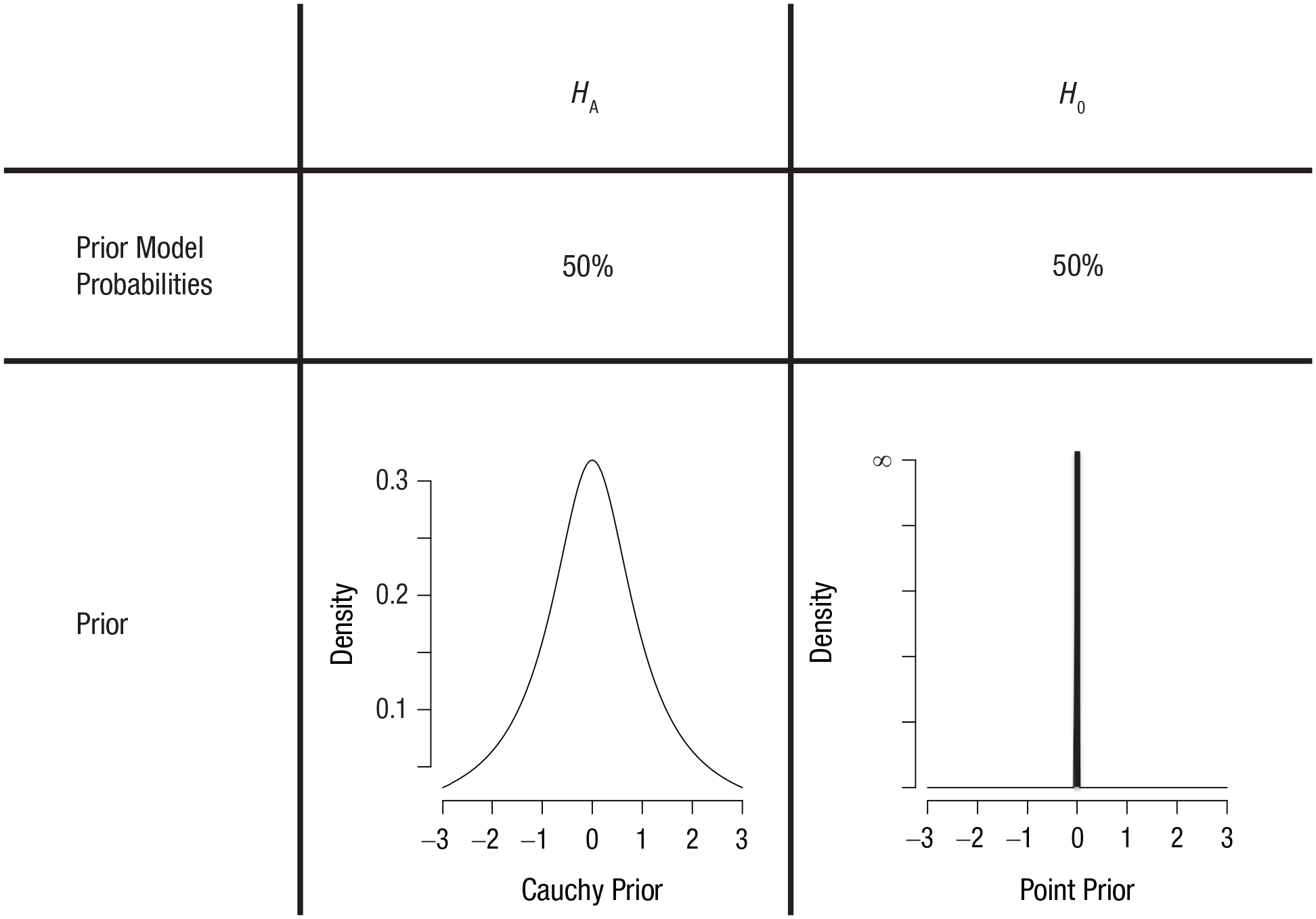
Prior distributions for the null hypothesis, H₀, that the effect size is exactly zero (i.e., a point prior) and an alternative hypothesis, H_A, that the effect size is distributed as a Cauchy distribution centered on zero with a scale parameter of $\sqrt{2} / 2$ .

So far, nothing of the above is specific to the default-Bayes-factor approach. What distinguishes this approach from any other approach to Bayesian hypothesis testing is the choice of the prior distribution for the effect-size parameter δ under the alternative hypothesis (i.e., the left side of Fig. 2). The chosen distribution for the prior given the alternative hypothesis is a Cauchy distribution centered on zero, usually with a scale parameter of $\sqrt{2} / 2$ (Morey et al., 2018). One may think of this prior as a standard normal distribution with fatter tails. The scale parameter is the upper and lower bound that encompasses 50% of the distribution. So, a Cauchy distribution centered on zero with a scale parameter of $\sqrt{2} / 2$ has 50% of the distribution between $- \sqrt{2} / 2$ and $\sqrt{2} / 2$ (or approximately −0.71 to 0.71).

The Cauchy prior has some desirable mathematical properties (see, e.g., Bayarri et al., 2012; Consonni et al., 2018), such as model-selection consistency (for data generated under a model, the corresponding Bayes factor should go to infinity as sample size goes to infinity), predictive matching (there should be a minimum sample size for which the Bayes factor is 1, such that models are indistinguishable), and information consistency (there should be a minimum sample size for which data that result in test statistics that go to infinity should have corresponding Bayes factors that also go to infinity). Other priors may share some of these desirable properties, but the Cauchy prior has caught on as the go-to choice because it satisfies them all and is relatively easy to specify and interpret.

As a perhaps more intuitive way to grasp why such a prior makes sense, we consider why the prior density should be relatively high for values closer to zero and why the distribution should be symmetrical. For most studies, it should be the case that an effect size of, say, δ = 10 is substantially less likely to be found than an effect size of, say, δ = 5. Similarly, δ = 5 should be less likely than δ = 2, which in turn should be less likely than δ = 0.8. Moreover, in the specific context of testing the null hypothesis that δ is zero, “the mere fact that we are seriously considering the possibility that it is zero may be associated with a presumption that if it is not zero it is probably small” (Jeffreys, 1961, p. 332). This accounts for the fact that the distribution is peaked instead of flat.

The second thing to bear in mind is that in the context of two-sided testing, negative effect sizes should be just as plausible as positive effect sizes, as every parameter can be flipped around such that the sign of the effect size switches (e.g., happiness can be relabeled unhappiness, Group 1 can be relabeled Group 2). This accounts for the fact that the distribution is symmetrical around zero.

You might wonder if it would not make more sense to have a distribution with two peaks, say, one at δ = 0.2 and one at δ = −0.2. Such a distribution would still be nonflat and symmetrical, but would incorporate the fact that the researchers probably have some intuition about the phenomena they want to investigate, such that small effects are more likely to be studied than null effects. The beauty of the Bayesian approach is that everyone is at liberty to pick their own prior distribution, the one they think best reflects the a priori knowledge of the field. The Cauchy prior described above is considered by many researchers to be a sensible default prior. It is relatively diffuse, reflecting the fact that the researcher is not willing to commit to very specific values of the effect-size parameter a priori. Such a prior will have a comparatively small influence on the posterior distribution, such that most of the diagnosticity comes from the likelihood of the data. We provide examples of the effect of choosing different kinds of priors in the section titled The Prior’s Influence on the Bayes Factor.

In the next subsection, we use simulation to generate data from the priors illustrated in Figure 2 under the null and alternative hypotheses to gain insight into the mechanics of the Bayes factor.

Simulation of Bayes factors

In the previous section, we explained that the Bayes factor is computed by taking the ratio of two probabilities: the probability of the data given the null hypothesis, P(data|H₀), and the probability of the data given the alternative hypothesis, P(data|H_A). In the section before that, we used simulation to draw samples from a prior distribution. In this section we combine these two ideas to obtain Bayes factors for data that have not yet been observed (see also Etz et al., 2018; Rouder, 2014). We illustrate this idea using a running example of Kim, an educational psychologist.

Kim is interested in examining whether a new program focused on more systematic rehearsal of learned topics leads to lasting increases in IQ scores among high-school students. She randomly selects 50 students from high schools in The Netherlands and has them enroll in her program (with permission from their teachers and parents, of course). Kim administers an IQ test to the 50 students directly before the program and half a year after the program. She is interested in whether there is a gain in the IQ score that lasts until half a year after the program.

Kim does not have any data yet, but we are going to use simulation to examine what data she might observe if the null hypothesis is true and what data she might observe if the alternative hypothesis is true. The first component of the Bayes factor that we focus on is P(data|H₀), the probability of the data given the null hypothesis. As indicated in the right side of Figure 2, the null hypothesis is a point null. This means that under the null hypothesis, the population effect size, δ, can only be zero. Using simulation, we can examine the sampling distribution of the sample effect size, Cohen’s d, when the null hypothesis is true and the sample size is 50. We use the following code to generate 10,000 sample effect sizes under the null hypothesis:



# Our sample size for each experiment
n = 50


# Number of simulated experiments to
# generate
nSims = 10000


# Create an empty (for now) vector in
# which to store sample effect sizes
Sample0 = c()


# Repeat nSims times: create data set ->
# compute effect size
for (i in 1:nSims)
{
 # Generate data set from N(0,1)
 data = rnorm (n, 0, 1)
 # Compute one sample effect size and
 # store in position i of the vector
 Sample0[i] = mean(data) / sd(data)
}

The resulting sample effect sizes are represented by the green histograms and density function in Figure 3. All four panels show the same data but with different granularity.

Fig. 3.

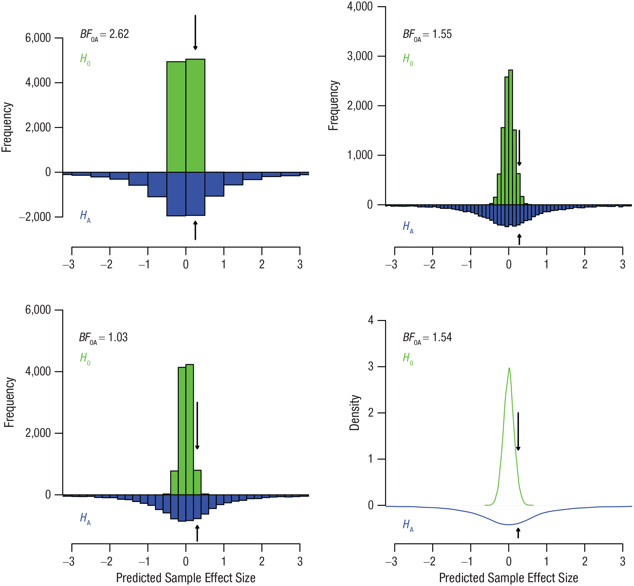
Sample effect sizes simulated from the prior distribution under the null hypothesis, H₀, and from the prior distribution under the alternative hypothesis, H_A. The arrows point to the bins that are the focus of the Bayes factor calculations discussed in the text. Note that we have plotted the negative of the frequency and density for the alternative hypothesis, which results in a reflection across the x-axis, for easier comparison. The same data are displayed in each of the panels, with increasingly more narrow bin widths from the top left to the bottom right. BF_0A = probability of the data under H₀ relative to the probability of the data under H_A.

Simulating data for the second component of the Bayes factor, P(data|H_A), is a little more involved. The complication comes from the fact that for the alternative hypothesis, we do not merely set δ to some fixed value. We instead specify a prior distribution for δ reflecting the fact that we do not yet know its true value. As indicated in the previous section, for this prior we use a Cauchy distribution centered on zero with scale of $\sqrt{2} / 2$ .

The way to incorporate the fact that we do not know the true value for δ is to add an additional step to the simulation. First, we sample a population effect size from the distribution of potential population effect sizes. In this case, the distribution of potential population effect sizes is dictated by the Cauchy prior. This extra step is implicit in the previous simulation for the null hypothesis because the population effect size is always the same (i.e., zero). Once we have generated this population effect size, we draw a data set of size 50 from this population effect size, just as in the simulation for the null hypothesis presented previously. We use the following code to generate 10,000 sample effect sizes under the alternative hypothesis:



# Create an empty (for now) vector to
# store sample effect sizes
SampleA = c()


# Repeat nSims times: sample a parameter ->
# create data set ->
# compute effect size
for (i in 1:nSims)
{
 # Generate a delta parameter (true
 # effect size) from the Cauchy dist.
 delta = rcauchy (1,0,scale=sqrt(2)/2)
 # Generate data set from N(delta, 1)
 data = rnorm (n, delta, 1)
 # Compute one sample effect size and
 # store in position i of the vector
 SampleA[i] = mean (data) / sd (data)
}

The resulting sample effect sizes are represented by the blue histograms and density function in Figure 3. The distributions of sample effect sizes under both hypotheses are called prior predictives (Ntzoufras, 2009). Now that we have distributions of hypothetical data under the null hypothesis and under the alternative hypothesis, the next step is to turn these into Bayes factors. Recall that a Bayes factor is nothing more than the ratio of the probability of the data under one hypothesis over the probability of the data under the other hypothesis. In other words, we can compare the green histograms with the blue histograms for a specific portion of the data, and the ratio of these two will be our Bayes factor.

Kim has not collected any data yet, but let us consider the scenario in which Kim has collected some data with a sample effect size, d, of 0.25. Under which hypothesis is this Cohen’s d more likely? In our simulated data, an exact value of 0.25 will not have occurred (at least not prior to rounding), but we can approximate the Bayes factor by binning the data. For instance, the top left panel of Figure 3 shows the data binned with a bin width of 0.5. We can get a very rough approximation of the Bayes factor for a sample d of 0.25 by dividing the number of times a d between 0 and 0.5 occurred under the null hypothesis and under the alternative hypothesis:



# Set the limits of our bin that is .5 wide
Bin = c(0, 0.5)


# Proportion of null-generated sample
# effect sizes within the bin limits
Nulls = mean (Sample0>Bin[1] & Sample0<Bin[2])


# Proportion of alternative-generated
# sample effect sizes in bin limits
Alts = mean (SampleA>Bin[1] & SampleA<Bin[2])


 # Approximate BF given by ratio of the
# two proportions
BF0A = Nulls / Alts

Essentially, what we are doing here is dividing the height of the green bar marked with an arrow by the height of the blue bar marked with an arrow. Running this script, we obtain a Bayes factor of 2.62. This means that if Kim will observe a sample effect size somewhere between 0 and 0.5, that data will have been slightly more likely under the null hypothesis than under the alternative hypothesis. Put differently, the null hypothesis predicts a sample d in the range of 0 and 0.5 more strongly than the alternative hypothesis does.

What happens if we make the bins more narrow? You can experiment by changing the values of the bin. The bottom left panel in Figure 3 examines the approximate Bayes factor for the bin from 0.2 to 0.4, and the top right panel examines the approximate Bayes factor for the bin from 0.2 to 0.3. For these bins in our specific samples, the approximate resulting Bayes factors are 1.03 and 1.55, respectively. For reference, the exact Bayes factor corresponding to a sample effect size of 0.25 and n = 50 is 1.54 (see the bottom right panel in Fig. 3).⁴ We see that even a bin with a width of 0.1 comes pretty close already.

What if Kim had collected data with a sample d of 0.75 instead of 0.25? Inspection of the histograms shows us that around value 0.75 on the x-axis, the blue bars are actually much larger than the green bars, indicating that this data are (much) more likely to occur under the alternative hypothesis than under the null hypothesis: The corresponding Bayes factor is over 6,000.

In the next two sections, we turn our attention to using simulation to approximate Bayes factors for data that are actually observed. In doing so, we substantially change the nature of our simulations. Before we generated many instances of data that were consistent with two different priors. In what follows, we zoom in on one specific data set that was actually observed and use simulation to draw samples from the posterior distribution. The samples from the prior and posterior distributions, in turn, can be used to obtain a Bayes factor.

Simulation of a Posterior Distribution

In the previous section, we simulated a wide range of data from the prior. We used the resulting simulated data sets to approximate Bayes factors for specific hypothetical data, should it have been observed. In this section, we assume that one specific data set has actually been observed, and we use simulation to explore the relationships among the posterior, the prior, and the Bayes factor (see Section 8.1 of Lee & Wagenmakers, 2013, for a similar demonstration). In other words, in the previous section we used simulation to generate multiple data sets that could be observed for a true parameter value. In the next two sections, we instead use simulation to explore how likely it is for a range of parameter values to have generated a single data set. So, in essence, we turn things around: Before, we looked at data that could have been observed given specific parameter values, and now we look at parameters that could have generated a specific data set.

Before we get to our example, a quick refresher of Bayes rule for estimation may be useful. Bayes rule states that the posterior density for an individual parameter value θ after the data have been seen is given by

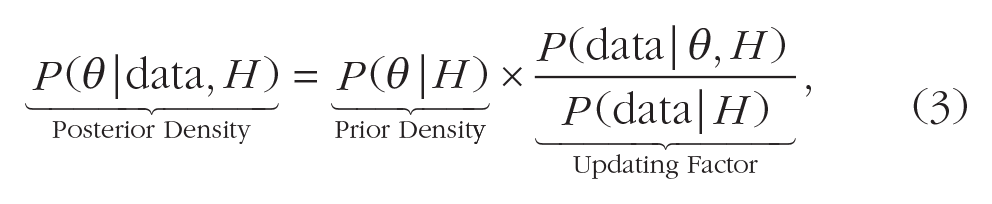
\underset{Posterior Density}{\underset{︸}{p (θ | data, H)}} = \underset{Prior Density}{\underset{︸}{p (θ | H)}} \times \underset{Updating Factor}{\underset{︸}{\frac{p (data | θ, H)}{p (data | H)}}},

(3)

where P(θ|H) is the prior density of θ, P(data|θ,H) is the likelihood for the data given the specific value for θ, and P(data|H) is the likelihood for the data that is a weighted average across each possible value of θ. The latter term is typically called marginal likelihood, as it is a likelihood in which one variable is collapsed over, or marginalized out. For example, say the probability of rain on any given day in January in The Netherlands is 30%: P(rain|January,Netherlands) = .3. Furthermore, say that the probability of rain on any given day in July in The Netherlands is 40%: P(rain|July,Netherlands) = .4. Assuming, for this simple example, that these are the only two months of the year, the marginal likelihood P(rain|Netherlands), in which the month variable is marginalized out, becomes (.3 + .4)/2, or .35; the number of days is identical in the two months, so that the weighted average of the probabilities is simply the mean. The likelihood we work with in the rest of these sections is P(data|δ,H), or the probability of the data given a specified population effect size, δ, as dictated by the t-test model. The marginal likelihood we work with in the rest of these sections is P(data|H), or the probability of the data given any population effect size, which is obtained by marginalization over the possible values of δ (weighted by the prior distribution).

The grouping of terms in Equation 3 makes it clear that the posterior density for a given parameter value θ is merely the prior density for that point multiplied by an updating factor. As we showed through simulation in the previous section, the likelihood and marginal likelihood (the terms making up the updating factor) are given by the heights of the prior predictive distributions at the point corresponding to the data, for a given parameter value θ (in our previous example, the null hypothesis, with value zero) and a weighted average over all θ values (in our previous example, the alternative hypothesis), respectively. Essentially, Bayes rule says that values of θ whose predictive distributions assign relatively high probability to the observed data get a bump in density, and those that assign relatively low probability to the data decrease in density.

In the following example, we use an overly simplistic data set. Our fictional data set consists of seven values: −2, −1, 0, 1, 2, 3, and 4. We are interested in testing if the population mean differs from zero. We can run this analysis simply in JASP by creating a .csv file with a column of these seven values and running a Bayesian one-sample t test (see Wagenmakers et al., 2018, for some JASP examples). The output is shown in the top panel of Figure 4.

Fig. 4.

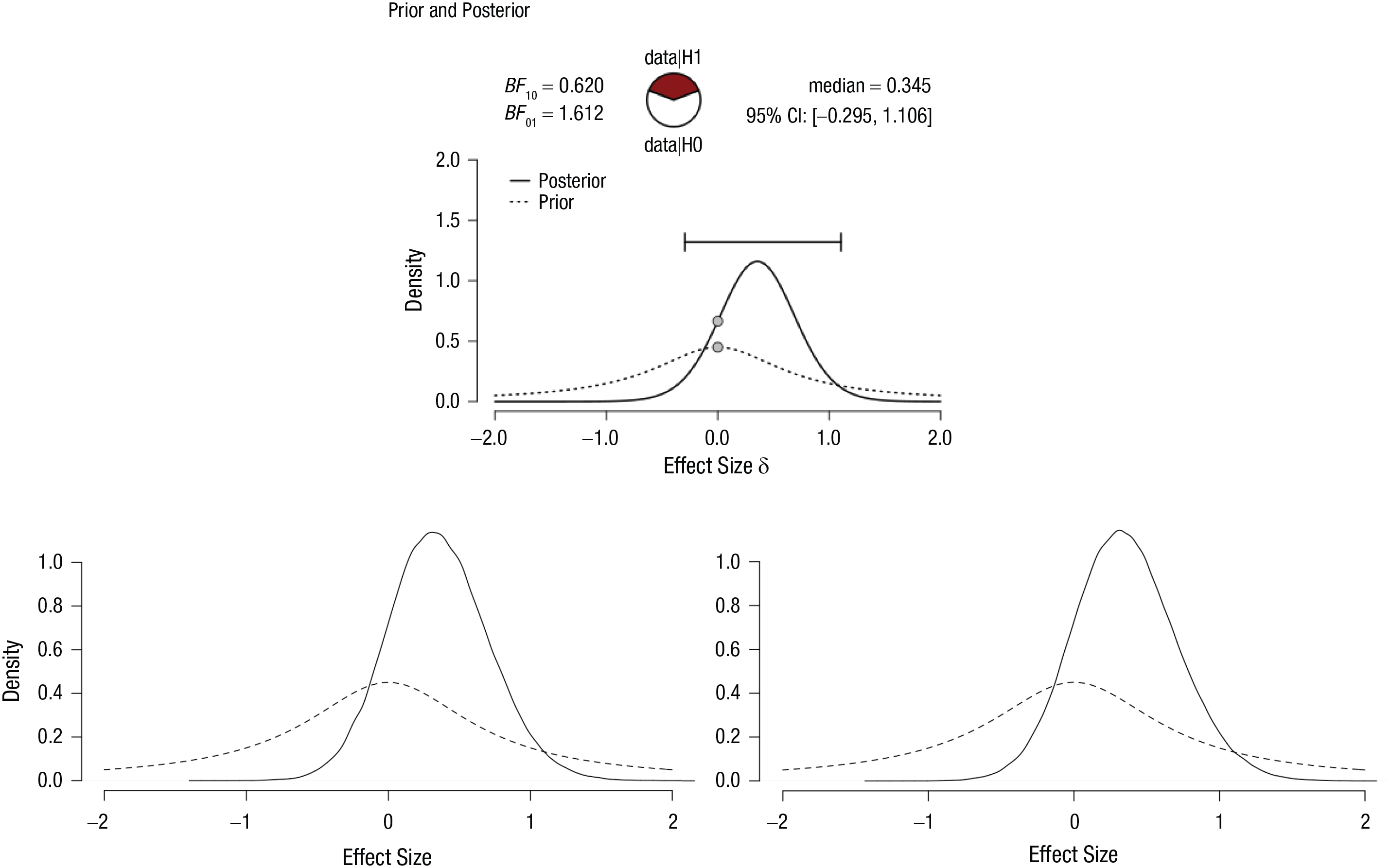
Posterior (and prior) distributions for the simple {−2, −1, 0, 1, 2, 3, 4} data set: the JASP output (top), the JAGS output based on the raw data (bottom left), and the JAGS output based on summary statistics (bottom right; see the appendix). In the top panel, the error bar indicates the 95% credible interval (CI), and the plotted points are the prior and posterior densities of δ evaluated at zero. BF₁₀ = Bayes factor for the probability of the data under the alternative hypothesis (H1) relative to the probability of the data under the null hypothesis (H0); BF₀₁ = Bayes factor for the probability of the data under H0 relative to the probability of the data under H1.

In the remainder of this section, we approximate what JASP computes directly (and, as a result, somewhat obscurely) with what a sampler can do more intuitively. For this to work, we need a working copy of JAGS (Plummer, 2003) in addition to R. We also need to install two R packages, R2jags (Su & Yajima, 2020) and (for later) polspline (Kooperberg et al., 2020). The following lines of code approximate the posterior distribution that JASP produced (the JAGS model itself is contained in the object JZSfulldata):



# Load the package R2jags, and
# interface between R and JAGS
library (R2jags)


# The data used for our sample
dat = -2:4


# Number of data points in the sample
n = length (dat)


# The following JZSfulldata object is
# a JAGS model string
# It will subsequently be used to
# specify the model in the jags()
# function below
JZSfulldata <- "model{
 # This for loop specifies the
 # likelihood for the data
 # ("How were the data from the sample
 # generated?")
 for (i in 1:n)
 {
  # Data point i is normally
  # distributed with mean mu and
  # precision invsigma2
  dat[i] ~ dnorm (mu, invsigma2)
 }


 # Next come prior distributions for
 # delta and invsigma2 parameters


 # Cauchy prior on delta (using the
 # t-dist. with 1 df)
 delta ~ dt (0, 2, 1)


 # Improper prior for sigma2
 # (approximating the Jeffreys′s prior)
 invsigma2 ~ dgamma (.00001, .00001)


 # Finally, transform back to the
 # variables mu and sigma
 sigma <- sqrt (1/invsigma2)
 mu <- delta * sigma
}"


# List of variables to be passed to
# JAGS (data and sample size)
Fulldata = list (dat = dat, n = n)


# This tells JAGS which parameters′
# samples we want to see when it
# finishes
JAGSparam = c("mu", "sigma", "delta")


# Finally, the jags() function calls
# JAGS to run the simulations as we
# specified
FitFulldata = jags (data = Fulldata,
 parameters.to.save = JAGSparam,
 n.thin = 1, n.iter = 20000, n.burnin =
  10000, n.chains = 1,
 model.file =
  textConnection(JZSfulldata))

The posterior distribution is ultimately obtained via compromise between the prior distribution and the information provided by the data through the likelihood (for an illustration, see Example 3 of Etz & Vandekerckhove, 2018). So now we need to provide prior distributions and a likelihood for the data. Starting with the likelihood, we assume that each data point comes from a normal distribution with unknown population mean µ and variance σ² (as we would with a traditional t test). Note that JAGS is a bit unorthodox when it comes to statistical software because it works with mean and precision parameters, the latter being the inverse of the variance. So rather than specifying a model using µ and σ or σ², we instead need to specify the model using µ and 1/σ². Thus, we specify a normal distribution with mean mu and precision invsigma2 in the code.

To complete our model, we need prior distributions for the parameters that are specified in our likelihood function. However, in the default Bayesian t test, one tests hypotheses using the standardized effect δ, calculated as µ/σ, so instead of specifying a prior for µ directly, we specify priors for δ and 1/σ² and then convert these to µ using µ = δ × σ (conversions take place in the last two lines of the model section of the code). Recall that the prior for δ is a Cauchy distribution centered on zero with a scale parameter of $\sqrt{2} / 2$ (equivalent to a t distribution with a scale of $\sqrt{2} / 2$ and 1 degree of freedom; see the left side of Fig. 2). The parameters required by JAGS for the t distribution are mean, precision (inverse of scale, squared), and degrees of freedom. Thus, the precision parameter of the δ prior we need to provide is the squared inverse of the scale: 2.

Finally, we need a prior for the precision, 1/σ². The formal prior used in the default Bayesian t test is known as the Jeffreys prior (Rouder et al., 2009), an improper prior because the area under the curve does not add up to 1.⁵ Unfortunately, improper priors are not allowed in JAGS. For our purposes, this prior is approximated nearly perfectly by an inverse gamma distribution with shape and scale parameters of 0.00001 (which is equivalent to a gamma distribution on σ² with shape and scale parameters of 0.00001). A visualization of a gamma distribution with shape and scale parameters of 0.00001 is provided in Figure 5.

Fig. 5.

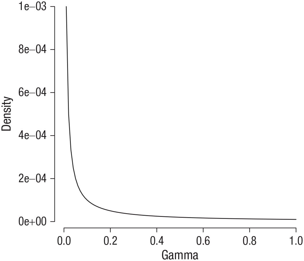
Gamma distribution with shape and scale parameters of 0.00001.

The remaining bit of code specifies the data and runs the JAGS sampler. Specifically, we draw 10,000 values from the posterior distribution (i.e., the difference between n.iter and n.burnin in the JAGS code). More would be possible, either by increasing the number of iterations or by running the simulation multiple times (i.e., increasing the number of chains), but for purposes of this example, 10,000 values offer more than enough precision to approximate the posterior distribution. We have chosen to run a large number of samples because that will allow us to approximate the Bayes factor that analytic methods provide more accurately. To plot the output of the sampler, we can use the following lines of code:



# Extract the mcmc samples JAGS
# generated
Fulldatamcmc = as.mcmc (FitFulldata)


# Pull out the mcmc samples for the
# delta parameter specifically
Fulldelta = Fulldatamcmc[[1]][,"delta"]


# Create a density plot of the posterior
# samples of delta
plot (density (Fulldelta, n = 4096),
 xlim = c(-2,2), bty = ′n′, axes = F,
 xlab = "Effect Size", ylab = "Density",
main = "")


# Create the axes
axis (1); axis (2, las = 1)


# Add the prior distribution of delta
# for comparison
curve (dcauchy (x, 0, sqrt(2)/2),
 from = −2, to = 2, lty = 2, add = T)

The resulting output is shown in the bottom left panel of Figure 4. The posterior shows us the probability density of different values of unknown population parameter δ, given the observed data set of {−2, −1, 0, 1, 2, 3, 4} under the alternative hypothesis. At first glance, the posterior distribution looks very similar to the one produced by JASP in the top panel. In the next section, we explore whether the Bayes factors for the analytic JASP approach and the approximate JAGS approach agree.

In the example, we specified a likelihood for each data point separately. It is entirely possible to summarize all the relevant characteristics of the data set using the sample test statistic t and put our likelihood on that instead. Such a specification is provided in the appendix.

With an approximation of the posterior distribution for our effect-size parameter δ under the alternative hypothesis in hand, we use this information in the next section to obtain the default Bayes factor.

Bayes Factor Visualization: The Savage-Dickey Method

We have used JAGS to great effect to obtain the posterior distribution for the effect-size parameter δ. We can now calculate a Bayes factor by taking the ratio of the prior and posterior densities of δ evaluated at zero, a technique known as the Savage-Dickey method (see, e.g., Wagenmakers et al., 2010). Conveniently, the Bayes factor is nothing more than an updating factor (see Equation 3), as it quantifies whether a parameter or hypothesis is more plausible after the data have been seen (quantified by the posterior) than before the data have been seen (quantified by the prior).

Although it can be shown mathematically why the Bayes factor can be represented as the ratio of the prior and posterior densities (see Box 1), in our opinion, understanding why the Savage-Dickey method works is not intuitive. In what follows, we use the simulation results from the previous section to explain the rationale behind the Savage-Dickey method.

Box 1.

The Savage-Dickey Density Ratio

The Savage-Dickey density ratio (often shortened to the Savage-Dickey ratio or Savage-Dickey method) is the ratio of posterior density to prior density for a parameter value (Dickey, 1971; Dickey & Lientz, 1970). The Savage-Dickey method is useful because it connects Bayes rule for hypothesis testing (Equation 2) with Bayes rule for estimation (Equation 3) and provides a way to “see” how large the Bayes factor is.

Consider the hypothesis-testing case when the null hypothesis, H₀, is nested within the alternative hypothesis, H_A, which means H₀ sets a parameter present in H_A to equal some predetermined value. The t test is one such example; H₀ restricts δ to take the value zero. In this scenario, P(data|δ = 0, H_A) will equal P(data|H₀) because H₀ is just H_A with the restriction δ = 0. Moreover, the same P(data|H_A) shows up in both the Bayes factor and the estimation updating factor. Thus, the Bayes factor testing whether δ = 0 equals the estimation updating factor at δ = 0. If we divide each side of Equation 3 by the prior density, we see the following result:

\underset{Savage - Dickey Ratio}{\underset{︸}{\frac{p (δ = 0 | data, H_{A})}{p (δ = 0 | H_{A})}}} = \underset{Updating Factor}{\underset{︸}{\frac{p (data | δ = 0, H_{A})}{p (data | H_{A})}}} = \underset{Bayes Factor}{\underset{︸}{\frac{p (data | H_{0})}{p (data | H_{A})}}} .

(4)

Hence, the Savage-Dickey ratio, the updating factor, and the Bayes factor are all equal, and we can conveniently visualize the Bayes factor as a comparison of the prior and posterior densities. When the posterior density is larger than the prior density, the Bayes factor will show evidence in favor of H₀, and when the posterior density is smaller than the prior density, the Bayes factor will show evidence against H₀.

However, it is important to note that this simple relationship between the Bayes factor and the Savage-Dickey density ratio can become more complicated in hypothesis-testing scenarios involving models with many interdependent parameters. In such cases, it is possible that the Savage-Dickey ratio and Bayes factor diverge by a positive scalar factor; that is, the ratio of posterior to prior density equals k, but the Bayes factor equals αk for some positive α. For technical explanations and examples of this phenomenon, see Heck (2019), Verdinelli and Wasserman (1995), and Wagenmakers et al. (in press, Section 6).

In order to gain some intuition with respect to the Savage-Dickey method, which is typically used to visualize the Bayes factor, we briefly move away from our original null hypothesis and alternative hypothesis. Specifically, we change our point null hypothesis (δ = 0) into an interval null hypothesis (and change our alternative hypothesis to all values outside the null interval). Say, for instance, that our null hypothesis is given by −0.5 < δ < 0.5, and our alternative hypothesis is given by |δ| > 0.5 (i.e., the remaining possible values of δ). This scenario is visualized in the top panel of Figure 6, in which the null hypothesis corresponds to the area between the vertical dashed lines.

Fig. 6.

Three different interval null hypotheses, indicated by the dashed vertical lines: −0.5 < δ < 0.5 (top panel), −0.25 < δ < 0.25 (middle panel), and −0.01 < δ < 0.01 (bottom panel). The interval null hypotheses are superimposed on the posterior and prior distributions obtained from JAGS in the previous section.

Recall that we can use Equation 2 to obtain the Bayes factor. Practically speaking, we need the areas of the posterior between the vertical lines and outside the vertical lines, and the areas of the prior between the vertical lines and outside of the vertical lines. With our JAGS samples in hand, we approximate the area of the posterior within the vertical lines by calculating the proportion of samples that fell within the vertical lines. The area outside the dashed lines is approximated by subtracting that proportion from 1 (recall that probability distributions sum to 1).

Because our prior distribution is an exact distribution, we can calculate the area of the prior within the vertical lines exactly. Code to calculate the four quantities needed is as follows:



# The max absolute value of delta
# under the null hypothesis
Margin = .5


# Area under the posterior for the
# null hypothesis
PostH0 = mean (Fulldelta>-Margin &
 Fulldelta<Margin)


# Area under the posterior for the
# alternative hypothesis
PostHA = 1 - PostH0


# Area under the prior for the null
# hypothesis
PriorH0 = pcauchy (Margin, 0,
 sqrt(2)/2) - pcauchy (-Margin, 0,
 sqrt(2)/2)


# Area under the prior for the
# alternative hypothesis
PriorHA = 1 - PriorH0


# Dividing the posterior odds by the
# prior odds gives the Bayes factor
BF0A = (PostH0/PostHA) / (PriorH0/
 PriorHA)

For our samples, we get a posterior area between the vertical lines of .67, but because the area was calculated using samples, you might get slightly different results. The area of the prior between the vertical lines is approximately .39. The resulting Bayes factor, BF_0A (the probability of the data under the null hypothesis relative to the probability of the data under the alternative hypothesis), would be calculated as $\frac{. 67}{1 - . 67} / \frac{. 39}{1 - . 39}$ , or approximately 3.20, so the relative support for the null hypothesis provided by the data is approximately 3.

Let us repeat this procedure, but now choosing a more narrow band around δ = 0 as our null hypothesis: −0.25 < δ < 0.25 (see the middle panel of Fig. 6). You can perform the calculation with us; all that is required is to change the Margin variable in the previous bit of code to reflect our new band of {−0.25, 0.25}. For our samples, we get a posterior area between the dashed lines of .36. The area of the prior between the dashed lines is approximately .22. Note that both areas are smaller than for the previous band, as they should be. The resulting Bayes factor is $\frac{. 36}{1 - . 36} / \frac{. 22}{1 - . 22}$ , or approximately 2.04.

We repeat this procedure one last time, now choosing a very narrow band around δ = 0 as our null hypothesis: −0.01 < δ < 0.01 (see the bottom panel of Fig. 6). For our samples, we get a posterior area between the dashed lines of .015. The area of the prior between the dashed lines is approximately .009. Note that the areas of both the prior and the posterior for the null hypothesis are now very small. The consequence of this is that the areas of both the prior and the posterior for the alternative hypothesis are close to 1.

We can exploit this to simplify our expression for the Bayes factor as follows: $B F_{0 A} = \frac{. 015}{1 - . 015} / \frac{. 009}{1 - . 009} \approx \frac{. 015}{009} \approx 1.64$ . That is, we can approximate the Bayes factor by dividing the area of the posterior for the null hypothesis by the area of the prior for the null hypothesis. We do not need to explicitly take into account the areas outside the vertical lines anymore! This approximation becomes better and better the more narrow our chosen band around δ = 0, providing we draw enough samples. In the limit, where we use the point null hypothesis δ = 0, dividing the height of the posterior for δ = 0 by the height of the prior for δ = 0 provides the exact Bayes factor. This method of obtaining the Bayes factor is called the Savage-Dickey method (see, e.g., Wagenmakers et al., 2010). We can calculate the Bayes factor using the Savage-Dickey method for our samples using the following bit of code:



# An R package that ′guestimates′ smooth
# densities based on data
library (polspline)


# Posterior density for null value
# under alt hypothesis
Post0underHA = dlogspline (0, logspline
 (Fulldelta))


# Prior density for null value under
# alt hypothesis
Prior0underHA = dcauchy (0, 0, sqrt(2)/2)


# The Savage Dickey ratio gives the
# Bayes factor
BF0A = Post0underHA / Prior0underHA

The logspline function essentially treats the sampled posterior distribution as if it were a proper density function and evaluates the density at δ = 0 as if the curve were smooth. Now that we are no longer working with interval hypotheses, the prior and posterior for the null hypothesis are no longer smooth continuations of the prior and posterior for the alternative hypothesis. Thus, our notation now refers to the prior and posterior density for the null value under the alternative hypothesis (i.e., the value above zero in the left side of Fig. 2). The resulting Bayes factor is 1.64 for our sample, which corresponds fairly well with the JASP output (see the top panel of Fig. 4, value of BF₀₁).

In this section and the previous one, we have attempted to visualize a way of obtaining Bayes factors that is an alternative to what happens behind the scenes when JASP calculates Bayes factors for a simple one-sample t-test design. One advantage of such a hands-on approximation is that it becomes quite simple to examine how strongly the choice of prior employed in the default-Bayes-factor approach influences the results obtained. We provide a few basic examples of how such an examination might be conducted in the next section.

The Prior’s Influence on the Bayes Factor

In the previous sections, we have seen the distinguishing feature of the JZS Bayes factor: the Cauchy prior. We have also seen how the Bayes factor can be calculated by (a) generating prior predictives under the null hypothesis and under the alternative hypothesis or (b) evaluating the prior and posterior distributions under the alternative hypothesis, evaluated at δ = 0, for an observed data set.

One reasonable question to ask is, how much does the choice of prior affect the Bayes factor? After all, sometimes multiple defensible nondefault priors can be specified in addition to or instead of a default prior (e.g., Dienes, 2019; Gronau et al., 2020; Jones & Johnson, 2014; Saunders et al., 2018). The sensitivity of Bayes factors to priors has been discussed previously by Liu and Aitkin (2008) and Vanpaemel (2010). In what follows, we demonstrate how to examine this sensitivity by calculating the Bayes factor for three alternative choices of prior that differ in increasing degrees from the Cauchy prior. The three other priors we examine are

A normal prior with a mean of 0 and variance of 1

A uniform prior with a range from −2 to 2

A bimodal normal prior, essentially a mixture of two normal priors with means of −2 and 2, respectively, and standard deviations of 1

The Cauchy, normal, uniform, and bimodal priors are visualized in the four columns of Figure 7.

Fig. 7.

Illustration of four different priors and their effect on posteriors and Bayes factors. From left to right, the priors are examples of Cauchy, normal, uniform, and bimodal distributions. The top row shows results for the small data set, and the bottom row shows results for the larger data set. See the text for details.

We run the sampler for our original data set {−2, −1, 0, 1, 2, 3, 4} and for a second, more substantial data set in which we drew 40 random samples from a normal distribution with a mean of 1 and standard deviation of 1. Code for running these models is provided below. Note that to keep the length of the code block manageable, we use the coding for the sample test statistic alluded to at the end of the section titled Simulation of a Posterior Distribution and explained in the appendix.



# Loads a module in JAGS that can deal
# with a mixture of distributions
load.module("mix")


# We create four different JAGS models
JZS <- list ("model{
 # The same likelihood is used for
 # each of the four models. We chose
 # a more efficient specification of
 # the likelihood (see appendix)
 tstat ~ dnt(delta * sqrt(n), 1, n-1)
 # Prior 1, the Cauchy prior
 delta ~ dt (0, 2, 1)
}",
 "model{
 tstat ~ dnt(delta * sqrt(n), 1, n-1)
 # Prior 2, the Normal prior
 delta ~ dnorm (0, 1)
}",
 "model{
 tstat ~ dnt(delta * sqrt(n), 1, n-1)
 # Prior 3, the Uniform prior
 delta ~ dunif (-2, 2)
}",
 "model{
 tstat ~ dnt(delta * sqrt(n), 1, n-1)
 # Prior 4, the bi-modal Normal prior
 delta ~ dnormmix (c(-2,2), c(1,1), c(1,1))
}")


# The two data sets used for our
# sample, put into a list
Dum = list (-2:4, rnorm (40, 1, 1))


# We create a list for our four
# models, each of which will
# be applied to two data sets
FitTstat = list ()


# A counter to put each result in a
# consecutive slot in the list
Count = 0


# Repeating variable specification for
# both data sets
for (i in 1:length(Dum))
{
 dat = Dum[[i]]
 # Sample mean
 m = mean (dat)
 # Number of data points
 n = length (dat)
 # Sample sd
 s = sd (dat)
 # t statistic
 tstat = (m/s)*sqrt(n)
 # JAGS variables
 Tstatdata = list (tstat = tstat, n = n)
 # JAGS parameter to be returned
 JAGStparam = c("delta")
 # Repeating running the jags()
 # function call for each model
 for (j in 1:length(JZS))
 {
  Count = Count + 1
  # Runs the simulations for each
  # data set and each model
  FitTstat[[Count]] = jags (data =
   Tstatdata,
   parameters.to.save = JAGStparam,
    n.thin = 1, n.iter = 20000,
   n.burnin = 10000, n.chains = 1,
   model.file =
    textConnection(JZS[[j]]))
 }
}

The resulting eight posterior distributions for the four different priors and two different data sets are shown in Figure 7.

For the remainder of this section, we discuss Bayes factors, indicating the probability of the data under the alternative hypothesis relative to the null hypothesis, that is, BF_A0 rather than BF_0A. BF_A0 can be converted to BF_0A by calculating 1/BF_A0. Looking first at the smaller, overly simplistic data set, we see that the difference in the Bayes factor between the Cauchy and normal priors is negligible (0.62 vs. 0.69). When we substantially change the prior to a uniform distribution, the Bayes factor decreases a bit, to 0.52. Finally, when we radically change the prior to a bimodal distribution, we get a completely different Bayes factor (about 0.17).

For the larger data set, we see that the choice of prior has less of an effect on the qualitative conclusions. The difference in the Bayes factor between the Cauchy and normal priors is small in relative terms (about 18,000 vs. about 15,000). When we substantially change the prior to a uniform distribution, the Bayes factor decreases a bit further, to about 13,000. Finally, when we radically change the prior to a bimodal distribution, our Bayes factor is about 17,000.

This small demonstration is not meant to be an exhaustive simulation, but it should provide the insight that prior distributions that are fairly diffuse (in the sense that they are spread over a wide range of values) and have somewhat similar shapes provide robust outcomes, even for small and strangely distributed data sets. As priors get more extreme, their effect on the Bayes factor becomes more pronounced, especially when data are sparse. Specifically, when priors are highly concentrated in regions of the parameter space that are largely inconsistent with the data, Bayes factors with extreme values can be expected. We recommend against using such extreme priors unless one has especially strong reasons to do so, such as copious and reliable previous data on the topic.

Conclusion

In this Tutorial, we have attempted to show in an intuitive manner how simulation studies can be employed to learn about statistical or mathematical concepts. We started out by providing code to simulate a normal prior distribution by sampling random values from this distribution.

Next, we transitioned to a description of Bayes factors for quantifying evidence in Bayesian testing. Our exposition was mainly conceptual, eschewing equations for intuition. We discussed a popular implementation, the JZS Bayes factor, which is the Bayes factor used in the BayesFactor package in R and the statistical freeware package JASP. We then used the idea of simulating from a prior distribution to show how generating data from priors under two hypotheses can be used to approximate Bayes factors for hypothetical, unobserved, data sets.

In the subsequent section, we took a different approach to approximating Bayes factors through simulation. It is not always easy to see for social scientists what happens in the black box of programs like the BayesFactor R package and the JASP software program. We approximated their operations by using simulations to approximate areas under posterior distributions. By effectively replacing the point null with a small interval around the null, we used simulations to approximate the exact Bayes factor provided by the Savage-Dickey method.

Finally, we harnessed the power of simulation to assess the effect of the choice of prior distribution on the Bayes factor for a modest selection of priors and two specific data sets. Such an approach can be implemented by researchers for their specific data set, but we caution against the use of extreme priors without proper a priori justification.

It is worth pointing out that the JZS Bayes factor is not the only popular implementation of the Bayes factor available. Other notable candidates include versions by Gönen et al. (2005), the online tool by Dienes (2008; see Singh, n.d.), and the minimum Bayes factor available in the pCalibrate R package (Ott & Held, 2017).

Note that we do not advocate using simulations for the calculation of Bayes factors to be reported in scientific articles. Whenever direct computation can be done, it should be preferred over approximating methods, such as simulations, much as experiments on a representative sample are unnecessary when the relevant information about the population is known.

With all of this said, in a world where the use of programs like R is increasingly common among researchers and students, we hope that viewing the JZS Bayes factor through the lens of a simulation approach increases understanding of this ever-more-popular vehicle for reporting the results of statistical testing.

Supplemental Material

sj-pdf-1-amp-10.1177_2515245920972624 – Supplemental material for Simulation Studies as a Tool to Understand Bayes Factors

Supplemental material, sj-pdf-1-amp-10.1177_2515245920972624 for Simulation Studies as a Tool to Understand Bayes Factors by Don van Ravenzwaaij and Alexander Etz in Advances in Methods and Practices in Psychological Science

Footnotes

Appendix: Simulation of a Posterior Distribution Using the t -Test Statistic

Code for obtaining the posterior using the t-test statistic is provided below:

The main changes compared with the example in the section titled Simulation of a Posterior Distribution are the following:

The noncentral t distribution may sound fancy, but in practice it boils down to the same thing as the likelihood on each individual data point, because the procedure behind computing a t-test statistic is based on the assumption that the data are normally distributed, which is made explicit in the likelihood for individual data points in the first JAGS model. Researchers can use this fact to their advantage when they wish to reanalyze published study results with a default-Bayes-factor approach and have access to the sample test statistics, but not the raw data. The procedure for a two-samples t test is very similar; in the JAGS model, the reader need only modify the likelihood to factor in the new noncentrality parameter δ × √(n₁ × n₂/(n₁ + n₂)) and degrees of freedom n₁ + n₂ − 2.

The code for plotting the output of the sampler is similar to the code for our example that used the raw data:

The output is presented in the bottom right panel of Figure 4.

Acknowledgements

We thank Quentin Gronau for helpful discussions about the manuscript.

Transparency

Action Editor: Daniel J. Simons

Editor: Daniel J. Simons

Author Contributions

D. van Ravenzwaaij and A. Etz jointly generated the idea for the study. D. van Ravenzwaaij wrote the R code used in the manuscript. A. Etz verified the accuracy of the R code. D. van Ravenzwaaij and A. Etz drafted the manuscript, and both authors critically edited it. Both authors approved the final submitted version of the manuscript.

ORCID iD

Don van Ravenzwaaij

Notes

References

Bayarri

M. J.

Berger

J. O.

Forte

García-Donato

(2012). Criteria for Bayesian model choice with application to variable selection. The Annals of Statistics, 40(3), 1550–1577.

Benjamin

D. J.

Berger

J. O.

Johannesson

Nosek

B. A.

Wagenmakers

E.-J.

Berk

Bollen

K. A.

Brembs

Brown

Camerer

Cesarini

Chambers

C. D.

Clyde

Cook

T. D.

De Boeck

Dienes

Dreber

Easwaran

Efferson

. . . Johnson

V. E.

(2018). Redefine statistical significance. Nature Human Behaviour, 2(1), 6–10.

Consonni

Fouskakis

Liseo

Ntzoufras

(2018). Prior distributions for objective Bayesian analysis. Bayesian Analysis, 13(2), 627–679.

Cumming

(2014). The new statistics: Why and how. Psychological Science, 25(1), 7–29.

Dickey

J. M.

(1971). The weighted likelihood ratio, linear hypotheses on normal location parameters. The Annals of Mathematical Statistics, 42(1), 204–223.

Dickey

J. M.

Lientz

B. P.

(1970). The weighted likelihood ratio, sharp hypotheses about chances, the order of a Markov chain. The Annals of Mathematical Statistics 41(1), 214–226.

Dienes

(2008). Understanding psychology as a science: An introduction to scientific and statistical inference. Macmillan International Higher Education.

Dienes

(2011). Bayesian versus orthodox statistics: Which side are you on? Perspectives on Psychological Science, 6(3), 274–290.

Dienes

(2019). How do I know what my theory predicts? Advances in Methods and Practices in Psychological Science, 2(4), 364–377.

10.

Etz

(2018). Introduction to the concept of likelihood and its applications. Advances in Methods and Practices in Psychological Science, 1(1), 60–69.

11.

Etz

Haaf

J. M.

Rouder

J. N.

Vandekerckhove

(2018). Bayesian inference and testing any hypothesis you can specify. Advances in Methods and Practices in Psychological Science, 1(2), 281–295. https://doi.org/10.1177/2515245918773087

12.

Etz

Vandekerckhove

(2018). Introduction to Bayesian inference for psychology. Psychonomic Bulletin & Review, 25(1), 5–34.

13.

Gelman

Jakulin

Pittau

M. G.

Y.-S.

(2008). A weakly informative default prior distribution for logistic and other regression models. The Annals of Applied Statistics, 2(4), 1360–1383.

14.

Gigerenzer

(2004). Mindless statistics. The Journal of Socio-Economics, 33(5), 587–606.

15.

Gönen

Johnson

W. O.

Westfall

P. H.

(2005). The Bayesian two-sample t test. The American Statistician, 59(3), 252–257.

16.

Gronau

Q. F.

Wagenmakers

E.-J.

(2020). Informed Bayesian t-tests. The American Statistician, 74(2), 137–143.

17.

Harlow

L. L.

Mulaik

S. A.

Steiger

J. H.

(1997). What if there were no significance tests? Erlbaum.

18.

Heck

D. W.

(2019). A caveat on the Savage-Dickey density ratio: The case of computing Bayes factors for regression parameters. British Journal of Mathematical and Statistical Psychology, 72(2), 316–333.

19.

The JASP Team. (2018). JASP (Version 0.8.6) [Computer software]. https://jasp-stats.org/

20.

Jeffreys

(1961). Theory of probability. Oxford University Press.

21.

Johnson

V. E.

(2013). Revised standards for statistical evidence. Proceedings of the National Academy of Sciences, USA, 110(48), 19313–19317.

22.

Jones

Johnson

W. O.

(2014). Prior elicitation: Interactive spreadsheet graphics with sliders can be fun, and informative. The American Statistician, 68(1), 42–51.

23.

Kass

R. E.

Wasserman

(1996). The selection of prior distributions by formal rules. Journal of the American Statistical Association, 91(435), 1343–1370.

24.

Kooperberg

Moler

Dongarra

(2020). polspline: Polynomial spline routines (Version 1.1.19) [Computer software]. Comprehensive R Archive Network. http://CRAN.R-project.org/package=polspline

25.

Kruschke

J. K.

(2014). Doing Bayesian data analysis: A tutorial with R, JAGS, and Stan. Elsevier Science.

26.

Kruschke

J. K.

Liddell

T. M.

(2018). Bayesian data analysis for newcomers. Psychonomic Bulletin & Review, 25(1), 155–177.

27.

Lee

M. D.

Wagenmakers

E.-J.

(2013). Bayesian cognitive modeling: A practical course. Cambridge University Press.

28.

Liu

C. C.

Aitkin

(2008). Bayes factors: Prior sensitivity and model generalizability. Journal of Mathematical Psychology, 52(6), 362–375.

29.

Morey

R. D.

Rouder

J. N.

(2011). Bayes factor approaches for testing interval null hypotheses. Psychological Methods, 16(4), 406–419.

30.

Morey

R. D.

Rouder

J. N.

Jamil

Urbanek

Forner

(2018). BayesFactor: Computation of Bayes factors for common designs (Version 0.9.12-4.1) [Computer software]. Comprehensive R Archive Network. https://CRAN.R-project.org/package=BayesFactor

31.

Ntzoufras

(2009). Bayesian modeling using WinBUGS. Wiley.

32.

Ott

Held

(2017). pCalibrate (Version 0.1-1) [Computer software]. Comprehensive R Archive Network. https://cran.r-project.org/web/packages/pCalibrate

33.

Plummer

(2003). JAGS: A program for analysis of Bayesian graphical models using Gibbs sampling. In Hornik

Leisch

Zeileis

(Eds.), Proceedings of the 3rd International Workshop on Distributed Statistical Computing (DSC 2003) (pp. 20–22). https://www.r-project.org/conferences/DSC-2003/Proceedings/Plummer.pdf

34.

R Development Core Team. (2020). R: A language and environment for statistical computing (Version 4.0.3) [Computer software]. R Foundation for Statistical Computing. http://www.R-project.org

35.

Rouder

J. N.

(2014). Optional stopping: No problem for Bayesians. Psychonomic Bulletin & Review, 21(2), 301–308.

36.

Rouder

J. N.

Speckman

P. L.

Sun

Morey

R. D.

Iverson

(2009). Bayesian t tests for accepting and rejecting the null hypothesis. Psychonomic Bulletin & Review, 16(2), 225–237.

37.

Saunders

Milyavskaya

Etz

Randles

Inzlicht

(2018). Reported self-control is not meaningfully associated with inhibition-related executive function: A Bayesian analysis. Collabra: Psychology, 4(1), Article 39. https://doi.org/10.1525/collabra.134

38.

Singh

(n.d.). Bayes factor (Dienes) calculator. https://medstats.github.io/bayesfactor.html

39.

Y.-S.

Yajima

(2020). R2jags: Using R to run ‘JAGS’ (Version 0.6-1) [Computer software]. Comprehensive R Archive Network. http://CRAN.R-project.org/package=R2jags

40.

van de Schoot

Winter

S. D.

Ryan

Zondervan-Zwijnenburg

Depaoli

(2017). A systematic review of Bayesian articles in psychology: The last 25 years. Psychological Methods, 22(2), 217–239.

41.

Vanpaemel

(2010). Prior sensitivity in theory testing: An apologia for the Bayes factor. Journal of Mathematical Psychology, 54(6), 491–498.

42.

van Ravenzwaaij

Cassey

Brown

S. D.

(2018). A simple introduction to Markov Chain Monte–Carlo sampling. Psychonomic Bulletin & Review, 25(1), 143–154.

43.

van Ravenzwaaij

Dutilh

Wagenmakers

E.-J.

(2012). A diffusion model decomposition of the effects of alcohol on perceptual decision making. Psychopharmacology, 219(4), 1017–2025.

44.

van Ravenzwaaij

Ioannidis

J. P. A.

(2017). A simulation study of the strength of evidence in the recommendation of medications based on two trials with statistically significant results. PLOS ONE, 12(3), Article e0173184. https://doi.org/10.1371/journal.pone.0173184

45.

van Ravenzwaaij

Ioannidis

J. P. A.

(2019). True and false positive rates for different criteria of evaluating statistical evidence from clinical trials. BMC: Medical Research Methodology, 19, Article 218. https://doi.org/10.1186/s12874-019-0865-y

46.

van Ravenzwaaij

Monden

Tendeiro

J. N.

Ioannidis

J. P. A.

(2019). Bayes factors for superiority, non-inferiority, and equivalence designs. BMC: Medical Research Methodology, 19, Article 71. https://doi.org/10.1186/s12874-019-0699-7

47.

van Ravenzwaaij

Wagenmakers

E.-J.

(2021). Advantages masquerading as ‘issues’ in Bayesian hypothesis testing: A commentary on Tendeiro and Kiers (2019). Manuscript submitted for publication.

48.

Verdinelli

Wasserman

(1995). Computing Bayes factors using a generalization of the Savage-Dickey density ratio. Journal of the American Statistical Association, 90(430), 614–618.

49.

Wagenmakers

E.-J.

(2007). A practical solution to the pervasive problems of p values. Psychonomic Bulletin & Re-view, 14(5), 779–804. https://doi.org/10.3758/BF03194105

50.

Wagenmakers

E.-J.

Gronau

Q. F.

Dablander

Etz

(in press). The support interval. Erkenntnis.

51.

Wagenmakers

E.-J.

Lodewyckx

Kuriyal

Grasman

R. P. P. P.

(2010). Bayesian hypothesis testing for psychologists: A tutorial on the Savage–Dickey method. Cognitive Psychology, 60(3), 158–159.

52.

Wagenmakers

E.-J.

Love

Marsman

Jamil

Verhagen

Selker

Gronau

Q. F.

Dropmann

Boutin

Meerhoff

Knight

Raj

van Kesteren

E.-J.

van Doorn

Šmíra

Epskamp

Etz

Matzke

. . . Morey

R. D.

(2018). Bayesian inference for psychology. Part II: Example applications with JASP. Psychonomic Bulletin & Review, 25(1), 58–76.

53.

Zellner

Siow

(1980). Posterior odds ratios for selected regression hypotheses. In Bernardo

J. M.

DeGroot

M. H.

Lindley

D. V.

Smith

A. F. M.

(Eds.), Bayesian statistics: Proceedings of the First International Meeting Held in Valencia (Spain) (pp. 585–603). University Press.

Supplementary Material

Please find the following supplemental material available below.

For Open Access articles published under a Creative Commons License, all supplemental material carries the same license as the article it is associated with.

For non-Open Access articles published, all supplemental material carries a non-exclusive license, and permission requests for re-use of supplemental material or any part of supplemental material shall be sent directly to the copyright owner as specified in the copyright notice associated with the article.

0.00 MB

0.26 MB