Sage Journals: Discover world-class research

Abstract

Accurate estimates of population effect size are critical to empirical science, for both reporting experimental results and conducting a priori power analyses. Unfortunately, the current most-popular measure of standardized effect size, partial eta squared ( ${\hat{η}}_{p}^{2}$ ), is known to have positive bias. Two less-biased alternatives, partial epsilon squared ( ${\hat{ε}}_{p}^{2}$ ) and partial omega squared ( ${\hat{ω}}_{p}^{2}$ ), have both existed for decades, but neither is often employed. Given that researchers appear reluctant to abandon ${\hat{η}}_{p}^{2}$ , this article provides a simple method for removing bias from this measure, to produce a value referred to as adjusted partial eta squared (adj ${\hat{η}}_{p}^{2}$ ). Some of the many benefits of adopting this measure are briefly discussed.

Keywords

population effect size eta squared partial eta squared unbiased estimates

The purpose of inferential statistics is to allow researchers to make accurate statements about populations on the basis of samples from those populations. One of the main threats to this process is bias, which can range from nonrepresentative sampling, to differences in how different subjects are treated, to confounds in the experimental design, to the choice of the statistic used to summarize the results. This article concerns the last of these issues and focuses on the bias in a popular measure of standardized effect size: partial eta squared ( ${\hat{η}}_{p}^{2}$ ; for an introduction, see, e.g., Richardson, 2011).¹

The main strength of ${\hat{η}}_{p}^{2}$ is that it can be interpreted in the same manner as a squared partial correlation coefficient (pr ²) from multiple linear regression: as the proportion of remaining variance in the dependent variable (i.e., the variance that cannot be “explained” by any other predictor) that can be “explained” by the predictor of interest (which would be a factor or interaction in experimental contexts). This commonality helps unify different approaches to theoretical questions, even allowing for direct comparisons between results from observational studies and those from laboratory experiments. Another strength is that ${\hat{η}}_{p}^{2}$ is a convenient starting point for a priori power analysis (see, e.g., Cohen, 1988), which is of high interest to all empirical scientists, especially those working in fields that may be suffering from a replication crisis (see, e.g., Ioannidis, 2005).

Unfortunately, ${\hat{η}}_{p}^{2}$ has notable bias: The value of this measure consistently overestimates the true population effect size (see Okada, 2013, for a recent discussion and clear demonstration). For example, assume the extreme situation in which the null hypothesis is exactly true—that is, the true means for the conditions are all the same. In this situation, under which the population effect size is clearly zero, the expected value of ${\hat{η}}_{p}^{2}$ is greater than zero. This is because even when the true means are all the same, the variance across the sample means will rarely, if ever, be zero. By random chance, one mean will be highest and another will be lowest, and these random differences will be “credited” to condition and cause the value of ${\hat{η}}_{p}^{2}$ to be greater than zero. Although the positive bias of ${\hat{η}}_{p}^{2}$ decreases as the true effect size increases, and also decreases as sample size increases, it is never zero.

In response to the positive bias of ${\hat{η}}_{p}^{2}$ , at least two alternative measures of standardized effect size have been proposed. The first is partial epsilon squared ( ${\hat{ε}}_{p}^{2}$ ; based on Kelley, 1935), and the second is partial omega squared ( ${\hat{ω}}_{p}^{2}$ ; Hays, 1963). Unfortunately, although both have been shown to have much less bias than ${\hat{η}}_{p}^{2}$ (e.g., Keselman, 1975; Okada, 2013) and at least one of these alternatives has been strongly recommended in most detailed, statistical discussions (e.g., Carroll & Nordholm, 1975; Grissom & Kim, 2012; Hays, 1963; Keppel, 1991; Maxwell & Delaney, 2004; see also Bakeman, 2005; Olejnik & Algina, 2003), neither of these alternatives has come close to supplanting ${\hat{η}}_{p}^{2}$ as the dominant measure of standardized effect size.²

In light of this, I take a different approach here. Instead of attempting to replace ${\hat{η}}_{p}^{2}$ as the go-to measure of standardized effect size, I provide a simple method for removing bias from this popular statistic. This approach to the problem of bias in ${\hat{η}}_{p}^{2}$ takes its cue from regression analysis (starting as far back as Ezekiel, 1930), in which one often sees both R² (which is known to have positive bias) and adjusted R² (adj R², which is the same measure with almost all of the bias removed). To emphasize and maintain the parallel with regression, as well as acknowledge one source for the idea, I refer to this statistic as adjusted partial eta squared, or adj ${\hat{η}}_{p}^{2}$ .

Before turning to the formula, I want to point out that the proposed method for removing bias from ${\hat{η}}_{p}^{2}$ produces values that are identical to those from one of the two existing alternatives, ${\hat{ε}}_{p}^{2}$ . In other words, the proposed process of first calculating or retrieving the value of ${\hat{η}}_{p}^{2}$ and then adjusting it to remove almost all of the bias is really a two-step method of calculating ${\hat{ε}}_{p}^{2}$ (see the appendix for an algebraic proof of this). The decision to emulate ${\hat{ε}}_{p}^{2}$ (instead of ${\hat{ω}}_{p}^{2}$ ) was based on two factors. First, the proposed method matches the well-established method that is used for regression: Mathematically, adj ${\hat{η}}_{p}^{2}$ is to ${\hat{η}}_{p}^{2}$ as adj R² is to R² (see Levine & Hullett, 2002). Second, in several comparisons (e.g., Carroll & Nordholm, 1975; Keselman, 1975; Okada, 2013), ${\hat{ε}}_{p}^{2}$ has been shown to be very close to completely unbiased, whereas ${\hat{ω}}_{p}^{2}$ has been found to have a small but consistent (negative) bias. Thus, modeling adj ${\hat{η}}_{p}^{2}$ on ${\hat{ε}}_{p}^{2}$ means that no new evidence of its superior accuracy is needed; what is already known about ${\hat{ε}}_{p}^{2}$ applies equally to adj ${\hat{η}}_{p}^{2}$ .

Calculating Adjusted Partial Eta Squared

Measures of standardized effect size have usually been presented in terms of sum-of-squares (SS) values (see, e.g., Maxwell, Camp, & Arvey, 1981), which can sometimes be daunting to nonstatisticians. For example, one formula for ${\hat{η}}_{p}^{2}$ (when expressed in a way that applies to all types of experimental designs—between subjects, within subjects, and mixed) is as follows:

{\hat{η}}_{p}^{2} = \frac{S S_{effect}}{S S_{effect} + S S_{error}} .

(1)

Similarly, the typical formula for ${\hat{ε}}_{p}^{2}$ involves a combination of SS values, a mean SS value (MS), and degrees of freedom:

{\hat{ε}}_{p}^{2} = \frac{S S_{effect} - d f_{effect} \times M S_{error}}{S S_{effect} + S S_{error}} .

(2)

The current approach starts with a much more user-friendly formula for ${\hat{η}}_{p}^{2}$ (Cohen, 1973, Equation 2; Levine & Hullett, 2002, Equation 3)—one that can easily be applied, after the fact, to the results from any F test, because the only required values are always available:

{\hat{η}}_{p}^{2} = \frac{F \times d f_{effect}}{F \times d f_{effect} + d f_{error}} .

(3)

Alternatively, if one only has access to the results from a t test, the formula is as follows:

{\hat{η}}_{p}^{2} = \frac{t^{2}}{t^{2} + d f_{error}} .

(4)

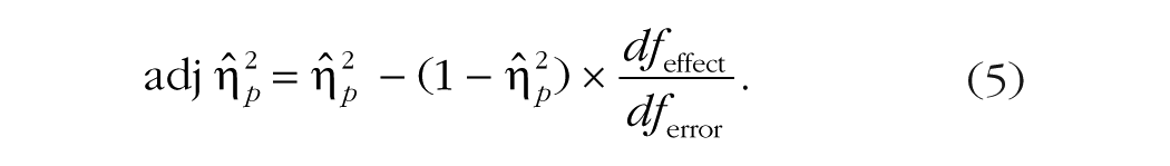
In the case of ${\hat{η}}_{p}^{2}$ , bias can also be moved from the calculation in a user-friendly manner (i.e., using only values that are readily available). The formula for adj ${\hat{η}}_{p}^{2}$ is this:

adj {\hat{η}}_{p}^{2} = {\hat{η}}_{p}^{2} - (1 - {\hat{η}}_{p}^{2}) \times \frac{d f_{effect}}{d f_{error}} .

(5)

If the value for ${\hat{η}}_{p}^{2}$ comes from a t test, then the value of df_effect is 1.

Note how expressing the method of adjustment in this manner—calculating the adjusted value as the original value minus an estimate of the bias—makes three (known) things quite clear: The amount of bias in ${\hat{η}}_{p}^{2}$ is proportional to the unexplained (error) variance, via 1 – ${\hat{η}}_{p}^{2}$ ; the amount of bias is also proportional to the number of predictors or conditions, via df_effect; and the bias is inversely proportional to the size of the sample, via df_error. Thus, for any fixed number of conditions, the most bias occurs when the true standardized effect size is small and the number of subjects or observations is low. Dangerously, these two things often co-occur in exploratory experiments, which makes a correction for bias particularly important in these situations.

To illustrate the importance of adjusting ${\hat{η}}_{p}^{2}$ to remove bias, I offer the following example. Assume a one-way between-subjects design with three conditions and 10 subjects per group (i.e., df_effect = 2 and df_error = 27). If the observed value of ${\hat{η}}_{p}^{2}$ is .200, then the value of adj ${\hat{η}}_{p}^{2}$ is .200 – (1 – .200)(2/27), which is only .141. Similarly, assuming a one-way within-subjects design with four conditions and 12 subjects (i.e., df_effect = 3 and df_error = 33), if the value of ${\hat{η}}_{p}^{2}$ of .400, then the value of adj ${\hat{η}}_{p}^{2}$ is .400 – (1 – .400)(3/33), which is .345. In short, the amount of bias that can (and should) be removed from ${\hat{η}}_{p}^{2}$ can be substantial.

With that said, it is important to note that adjusting ${\hat{η}}_{p}^{2}$ deals only with bias in the narrow, technical, statistical sense (which is defined as the difference between the expected value of an estimator and the true population value). It does not, for example, remove any of the problems associated with design confounds, demand characteristics, experimenter bias, or various questionable research practices, such as the unjustified omission of some subjects’ data. Nor does the use of adj ${\hat{η}}_{p}^{2}$ address the problems of p-hacking or publication bias. The present method is designed only to correct the statistical problems that are inherent to using (unadjusted) ${\hat{η}}_{p}^{2}$ .

Adopting Adjusted Partial Eta Squared

One possible criticism of adj ${\hat{η}}_{p}^{2}$ is that it is not anything new—that no new label or formula is needed or warranted, given that adj ${\hat{η}}_{p}^{2}$ is mathematically equivalent to ${\hat{ε}}_{p}^{2}$ (see the appendix). There are two counterarguments to this criticism. First, ${\hat{ε}}_{p}^{2}$ has had 80+ years to make inroads (and ${\hat{ω}}_{p}^{2}$ has had 50+ years), but ${\hat{η}}_{p}^{2}$ remains dominant, despite being known to be biased. It is time to try a different approach—one that does not ask researchers to completely abandon their favorite measure. Second, retaining ${\hat{η}}_{p}^{2}$ as one measure of standardized effect size, while also providing a simple method for removing almost all of the bias, may cause more researchers to acknowledge the bias in ${\hat{η}}_{p}^{2}$ and, therefore, be motivated to do something about it. The proposed formula for adj ${\hat{η}}_{p}^{2}$ makes explicit the sources of the bias, while the mere existence of a formula for adjusting ${\hat{η}}_{p}^{2}$ acts as a reminder that the (uncorrected) measure really is biased.

Another possible criticism of adj ${\hat{η}}_{p}^{2}$ (when compared with, e.g., additional attempts to encourage the use of either ${\hat{ε}}_{p}^{2}$ or ${\hat{ω}}_{p}^{2}$ ) is that it may add confusion. Instead of a single measure of standardized effect size, there would be two: one with noticeable (positive) bias and one that is almost completely unbiased. The counterargument is that highly biased and almost unbiased measures—R² and adj R², respectively—have coexisted in the regression literature for decades with little or no problem. In fact, having the two measures side by side will act as a reminder of the issue of bias, which can be crucial in certain contexts, such as power analysis, in which overestimates of the population effect size lead to underpowered experiments and possible failures to replicate. Furthermore, anything that emphasizes the commonalities between analysis of variance and regression could be of some benefit, as anyone who already understands the purpose of adj R² will immediately see the value of adj ${\hat{η}}_{p}^{2}$ .

It should be noted, however, that removing bias from ${\hat{η}}_{p}^{2}$ has the consequence of increasing its variability (see Albers & Lakens, 2018, for a clear demonstration). The amount by which the variability is increased depends entirely on the ratio of the degrees of freedom (in this case, the size of the effect does not play a role), but it can be nonnegligible. Assuming, for example, a one-way three-level between-subjects design with only 10 subjects per group (i.e., a ratio of degrees of freedom of 2/27), the variance of any set of adj ${\hat{η}}_{p}^{2}$ values will be 15% higher than the variance of the corresponding (uncorrected) ${\hat{η}}_{p}^{2}$ values. Moreover, when the true population effect size is small and the size of the sample is small, specific values of adj ${\hat{η}}_{p}^{2}$ can be negative, because of sampling error, and these cannot be “rounded up” to zero without introducing a new form of positive bias (see Okada, 2017). To put this in technical terms, although adj ${\hat{η}}_{p}^{2}$ is much less biased than ${\hat{η}}_{p}^{2}$ , it is also a bit less efficient.

More generally, it is important to recognize that having the least biased estimate of some population parameter is only a part of the story. For a more complete picture, some associated estimate of sampling error, such as a confidence interval, should also be calculated. Although this is quite complicated in the case of a population effect size, as it requires the use of the noncentral F distribution (e.g., Smithson, 2001; Steiger, 2004; see Cumming & Finch, 2001, for an introduction), calculation of a confidence interval is highly recommended. If nothing else, a confidence interval will provide researchers with a very clear warning as to the dangers of estimating the population effect size from a small sample.

To end on a positive, note that switching to a less biased estimate of population effect size will prevent a much thornier problem that arises when the results from experiments with very different numbers of subjects are compared. Recall that the amount of bias in ${\hat{η}}_{p}^{2}$ is inversely proportional to df_error, which is highly dependent on the number of observations. If two experiments involve the same manipulations and measures (as would be the case for exact replications), but one experiment has twice as many subjects as the other, then the larger study is expected to produce a slightly smaller ${\hat{η}}_{p}^{2}$ , because of less positive bias in the estimate. Thus, all exact replications with increased numbers of subjects are expected to produce smaller values of ${\hat{η}}_{p}^{2}$ than the original experiment, especially when the population effect size is small. This shrinkage of ${\hat{η}}_{p}^{2}$ going from a smaller to a larger experiment will occur even in the absence of any questionable research practices (John, Loewenstein, & Prelec, 2012); it is a consequence of the different amounts of bias. In contrast, because adj ${\hat{η}}_{p}^{2}$ is almost completely unbiased, the values for larger and smaller experiments are expected to be almost exactly the same.

In summary, an accurate estimate of population effect size is critical to many steps in the scientific process, from a priori power analysis to the comparison of new results with previous experiments and studies. Sadly, the current most-popular measure of standardized effect size— ${\hat{η}}_{p}^{2}$ —has notable (positive) bias. Fortunately, a simple method can remove almost all of the bias from this measure. This method of adjustment, which produces a value here named adjusted partial eta squared, adj ${\hat{η}}_{p}^{2}$ , can (and should) be applied to all estimates of population effect size.

Footnotes

Appendix: Proof of the Equivalence of Adjusted Partial Eta Squared and Partial Epsilon Squared

Start with the following user-friendly formula for ${\hat{η}}_{p}^{2}$ (Cohen, 1973, Equation 2):

(A1)

{\hat{η}}_{p}^{2} = \frac{F \times d f_{effect}}{F \times d f_{effect} + d f_{error}} .

The proposed formula for correcting this value for bias is

(A2)

adj {\hat{η}}_{p}^{2} = {\hat{η}}_{p}^{2} - (1 - {\hat{η}}_{p}^{2}) \times \frac{d f_{effect}}{d f_{error}} .

Inserting Equation A1 into Equation A2 creates a one-step method of calculating adj ${\hat{η}}_{p}^{2}$ :

(A3)

\begin{array}{l} adj {\hat{η}}_{p}^{2} = \frac{F \times d f_{effect}}{F \times d f_{effect} + d f_{error}} - \\ (1 - \frac{F \times d f_{effect}}{F \times d f_{effect} + d f_{error}}) \times \frac{d f_{effect}}{d f_{error}} . \end{array}

Next, create a common denominator within the parentheses using identity:

(A4)

\begin{array}{l} adj {\hat{η}}_{p}^{2} = \frac{F \times d f_{effect}}{F \times d f_{effect} + d f_{error}} - (\begin{array}{l} \frac{F \times d f_{effect} + d f_{error}}{F \times d f_{effect} + d f_{error}} - \\ \frac{F \times d f_{effect}}{F \times d f_{effect} + d f_{error}} \end{array}) \times \\ \frac{d f_{effect}}{d f_{error}} . \end{array}

Simplify the parenthetical by subtraction:

(A5)

\begin{array}{l} adj {\hat{η}}_{p}^{2} = \frac{F \times d f_{effect}}{F \times d f_{effect} + d f_{error}} - \\ \frac{d f_{error}}{F \times d f_{effect} + d f_{error}} \times \frac{d f_{effect}}{d f_{error}} . \end{array}

Then multiply:

(A6)

adj {\hat{η}}_{p}^{2} = \frac{F \times d f_{effect}}{F \times d f_{effect} + d f_{error}} - \frac{d f_{effect}}{F \times d f_{effect} + d f_{error}} .

Then subtract:

(A7)

adj {\hat{η}}_{p}^{2} = \frac{F \times d f_{effect} - d f_{effect}}{F \times d f_{effect} + d f_{error}} .

Then simplify:

(A8)

adj {\hat{η}}_{p}^{2} = \frac{(F - 1) \times d f_{effect}}{F \times d f_{effect} + d f_{error}} .

The expression on the right side of the equal sign in Equation A8 is mathematically equivalent to a user-friendly formula for ${\hat{ε}}_{p}^{2}$ (see, e.g., Carroll & Nordholm, 1975, Equation 11). Therefore,

(A9)

adj {\hat{η}}_{p}^{2} = {\hat{ε}}_{p}^{2} .

It is worth noting that Equation A8 provides a convenient method of calculating adj ${\hat{η}}_{p}^{2}$ directly from the results of an F test, without first finding the value of ${\hat{η}}_{p}^{2}$ . (If you start from a t test instead, recall that F = t² and that df_effect for a t test is 1.)

Acknowledgements

I thank Joe Hilgard, Andrew Hollingworth, Cathleen Moore, Kensuke Okada, Teresa Treat, and one anonymous reviewer for their helpful comments, and Daniel Q. Naiman for first teaching me about unbiased estimators.

Action Editor

Simine Vazire served as action editor for this article.

Author Contributions

J. T. Mordkoff is the sole author of this article and is responsible for its content.

Declaration of Conflicting Interests

The author(s) declared that there were no conflicts of interest with respect to the authorship or the publication of this article.

Open Practices

Open Data: not applicable

Open Materials: not applicable

Preregistration: not applicable

Notes

References

Albers

Lakens

(2018). When power analyses based on pilot data are biased: Inaccurate effect size estimators and follow-up bias. Journal of Experimental Social Psychology, 74, 187–195.

Bakeman

(2005). Recommended effect size statistics for repeated measures designs. Behavior Research Methods, 37, 379–384.

Carroll

R. M.

Nordholm

L. A.

(1975). Sampling characteristics of Kelley’s ε and Hays’ ω. Educational and Psychological Measurement, 35, 541–554.

Cohen

(1973). Eta-squared and partial eta-squared in fixed factor ANOVA designs. Educational and Psychological Measurement, 33, 107–112.

Cohen

(1988). Statistical power analysis for the behavioral sciences (2nd ed.). Mahwah, NJ: Erlbaum.

Cumming

Finch

(2001). A primer on the understanding, use, and calculation of confidence intervals that are based on central and noncentral distributions. Educational and Psychological Measurement, 61, 532–574.

Ezekiel

M. J. B.

(1930). Methods of correlational analysis. New York, NY: Wiley.

Grissom

R. J.

Kim

J. J.

(2012). Effect sizes for research: Univariate and multivariate applications (2nd ed.). New York, NY: Taylor & Francis.

Hays

W. L.

(1963). Statistics for psychologists. New York, NY: Holt, Rinehart, and Winston.

10.

Ioannidis

J. P. A.

(2005). Why most published research findings are false. PLOS Medicine, 2(8), Article e124. doi:10.1371/journal.pmed.0020124

11.

John

L. K.

Loewenstein

Prelec

(2012). Measuring the prevalence of questionable research practices with incentives for truth telling. Psychological Science, 23, 524–532.

12.

Kelley

T. L.

(1935). An unbiased correlation ratio measure. Proceedings of the National Academy of Sciences, USA, 21, 554–559.

13.

Keppel

(1991). Design and analysis: A researcher’s handbook. Englewood Cliffs, NJ: Prentice Hall.

14.

Keselman

(1975). A Monte Carlo investigation of three estimates of treatment magnitude: Epsilon squared, eta squared, and omega squared. Canadian Psychological Review, 16, 44–48.

15.

Levine

T. R.

Hullett

C. R.

(2002). Eta squared, partial eta squared, and misreporting of effect size in communication research. Human Communication Research, 28, 612–625.

16.

Maxwell

S. E.

Camp

C. J.

Arvey

R. D.

(1981). Measures of strength of association: A comparative examination. Journal of Applied Psychology, 66, 525–534.

17.

Maxwell

S. E.

Delaney

H. D.

(2004). Designing experiments and analyzing data: A model comparison perspective (2nd ed.). Mahwah, NJ: Erlbaum.

18.

Okada

(2013). Is omega squared less biased? A comparison of three major effect size indices in one-way ANOVA. Behaviormetrika, 40, 129–147.

19.

Okada

(2017). Negative estimate of variance-accounted-for effect size: How often it is obtained, and what happens if it is treated as zero. Behavior Research Methods, 49, 979–987.

20.

Olejnik

Algina

(2003). Generalized eta and omega squared statistics: Measures of effect size for some common research designs. Psychological Methods, 8, 434–447.

21.

Richardson

J. T. E.

(2011). Eta squared and partial eta squared as measures of effect size in educational research. Educational Research Review, 6, 135–147.

22.

Smithson

(2001). Correct confidence intervals for various regression effect sizes and parameters: The importance of noncentral distributions in computing intervals. Educational and Psychological Measurement, 61, 605–632.

23.

Steiger

J. H.

(2004). Beyond the F test: Effect size confidence intervals and tests of close fit in the analysis of variance and contrast analysis. Psychological Methods, 9, 164–182.