Addressing Unusual Assay Variability with Robust Statistics

Abstract

Well-behaved, in vitro bioassays generally produce normally distributed values in their primary (efficacy) data. Accordingly, the best practices for statistical analysis are well documented and understood. However, assays may occasionally display unusually high variability and fall outside the assumptions inherent in these standard analyses. These assays may still be in the optimization phase, in which the source of variation could be identified and addressed. They might also represent the best available option to address the biological process being examined. In these cases, the use of robust statistical methods may provide a more appropriate set of tools for both data analysis and assay optimization. This article provides guidance on best practices for the use of robust statistical methods for the analysis of bioassay data as an alternative to standard methods. Impacts on experimental design and interpretation will be discussed.

Introduction

In vitro bioassays are an essential component for biomedical research, and best practices for the development, validation, and analysis of these assays are well documented.^1–3 Primary data are often measured in arbitrary units and can vary due to both environmental changes and differences in instrument performance. The initial step in data analysis is to normalize the data to control for variation within and between experiments as well as to add a more easily interpretable biological context. This is often done by converting the raw data to a percentage activity scale using 2 controls to represent no effect (0% activity) and full (100%) activity. Three controls may also be used for assays that are intended to measure both stimulation and inhibition simultaneously, with the compounds representing 100% activity and -100% activity. For plate-based assays, it is also assumed that the variation in the measurements within a plate will be less than that between plates within an experiment or across multiple experiments.

Summary statistics such as mean and standard deviation are commonly used and appropriate for these assays. However, these statistics assume a normal population distribution for the measurements and can be significantly affected by extreme outliers or skewness, especially when the sample size is small (n < 30). Although increases in the well densities of microtiter plates have significantly reduced the cost of testing and increased the capacity, most test samples are still tested in singlets or at low replication (n ≤ 3), although replication rates for the control wells have risen significantly with increasing plate densities. In addition, assay performance statistics such as minimum significant difference and minimum significant ratio ⁴ can provide information about the overall reproducibility of assay efficacy or potency measurements.

Robust statistics, ⁵ such as median, median absolute deviation (MAD), and quartiles, are based on the rank order of the data and are less sensitive to the effects of extreme outliers. This study explores the impact of the use of robust statistics in the analysis of 2 assays that were designed to investigate the potential recruitment of the E3 ubiquitin ligase complex to affect the protein homeostasis ⁶ of specific targets (Tgt1 or Tgt2). Each of these assays was found to consistently exhibit a small percentage of extreme, random outliers that made it difficult to resolve intermediate degraders using traditional analysis techniques. This article examines and compares the use of nonrobust versus robust statistical summaries in terms of overall assay performance measures and the accuracy of the screening results.

Materials and Methods

Two protein homeostasis targets were identified (Tgt1 and Tgt2) as potential candidates for directed degradation by the E3ligase ubiquitination pathway. Each target protein was modified to contain a tagged domain that would later be used to determine relative protein levels via a DiscoveRx fragment complementation assay technology. The 2 targets were stably expressed in different cell lines and assessed separately, each as its own assay.

Tgt1 was transformed into an adherent cell line that was grown in media (DMEM, 10% heat-inactivated fetal bovine serum [FBS], 1× pen/strep), trypsin treated, and resuspended in media to 0.2 × 10⁶ cells/mL prior to plating and assessment in assay 1. Tgt2 was transformed into a suspension cell line that was grown in media (RPMI-1640, 10% heat-inactivated FBS, 25 mM Hepes, 1 mM Na pyruvate, 1 mM glutamine, 1× nonessential amino acid, 0.1% pluronic F-68, 1× pen/strep, 5 µg/mL BLAST) and concentrated to 0.2 × 10⁶ cells/mL prior to plating and assessment in assay 2. From this point, both cell lines were treated similarly with respect to assay conditions.

DiscoveRx Degradation Assay

The DiscoveRx (Freemont, CA) InCELL Hunter (catalog No. 96-0002) fragment complementation assay was used to monitor luminescent signal associated with a protein of interest in each cell line, as illustrated in Figure 1 . Cell lines stably expressing an ePL-tagged protein were dispensed into a 1536-well plate (Corning No. 3727 or Greiner No. 782075) at 1000 cells/well. The plates were either empty (training sets) or prespotted with compound (DRC). Compounds were dispensed using an ATS-100 acoustic transfer system (EDC Biosystems, San Jose, CA), as a 22-point dose-response curve using twofold dilutions starting at an assay concentration of 10 µM and going down to 0.00015 µM in DMSO. DMSO was used as the negative control, and a luciferase-specific inhibitor was used as a positive control. All wells were normalized to 0.2% DMSO for final assay conditions. Assay plates were incubated at 37 °C with 5% CO₂ for 24 h after application of the cells. After incubation, 5 µL of the InCELL Hunter Detection Reagent Working Solution was added to each well and incubated at room temperature, protected from light. After 1 h, luminescence was read on a ViewLux luminometer (PerkinElmer, Waltham, MA).

Figure 1.

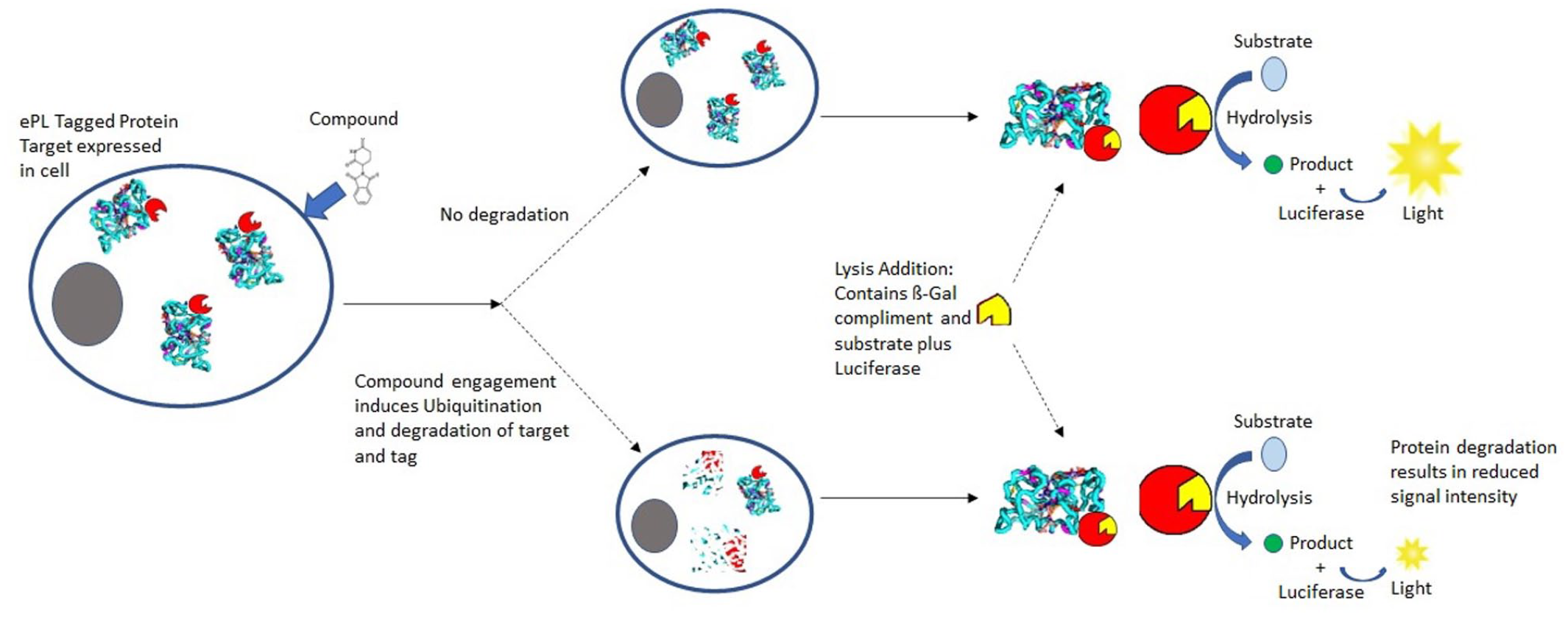
An illustration of the use of the DiscoveRx InCELL Hunter fragment complementation assay to monitor relative protein abundance.

Data Analysis

Typical (nonrobust) normalization of assay data per plate uses the mean response value of the vehicle control wells, C₀, and the full activity control wells, C₁, as follows:

$$Y^{\prime }=100\times \frac{\left(Y-C_0\right)}{C_1-C_0}$$

Our robust analysis used the control medians in place of the means. For the robust Z-factor, medians replaced means, and the MAD replaced the standard deviation. ⁷

Data were analyzed using R. Primary data and the analysis code are available on GitHub at github.com/Jeff-Qualsci/RobustAssayAnalysis.

Results

The vehicle control (TOTB), which represents both the maximum luminescence values in the assay and 0% activity for the within-plate normalization, was observed to have the most variability. A series of 1536-well uniformity plates, with all wells treated with vehicle control, were run across multiple days and multiple plates per day. Two different manufactured microtiter plates were run to both explore the vehicle control issue and determine if it might be related to a specific plate type. Figure 2 illustrates the problem for both assays. The scale of raw data varies significantly across both experiments and individual plates, so the well data were rescaled to the plate medians to control for this. Median scaling was chosen because it is less affected by any outliers. Box plots emphasize the outlier data points, while illustrating the distribution of the entire data set. ⁸ The distribution of outliers is often skewed either above or below the plate means, suggesting the data are not normally distributed. No significant differences were observed between the 2 plate types.

Figure 2.

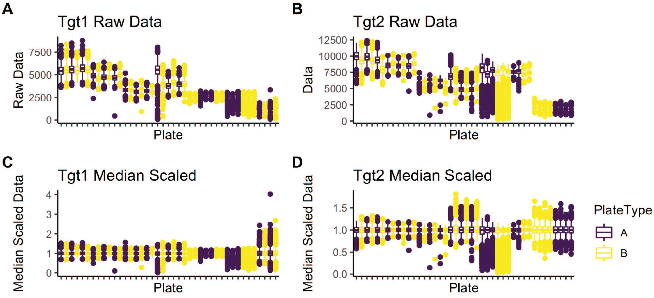
TOTB plate uniformity data. Box plots of all plate wells as both raw data (A, B) and scaled to the plate medians. Outliers are represented as points beyond the range of the whiskers.

The primary goal of any assay is to test multiple samples or conditions to learn about the biological system. A series of dose-response plates were tested in two experiments for each assay with seven replicate plates per experiment. Each plate contained 64 wells of both the vehicle and active (NSB) controls, which were then used to normalize all the data within each plate to percentage activity. The control well data for each plate is presented in Figure 3 . As with the uniformity plates, the extreme outliers are still seen in the normalized TOTB controls and can span the entire biological range of the assay. Despite having 64 replicates for each control, several plates show significant differences between the mean and median values for the TOTB control wells within a plate. In these cases, the normalization would yield different percentage activities using the median instead of the mean.

Figure 3.

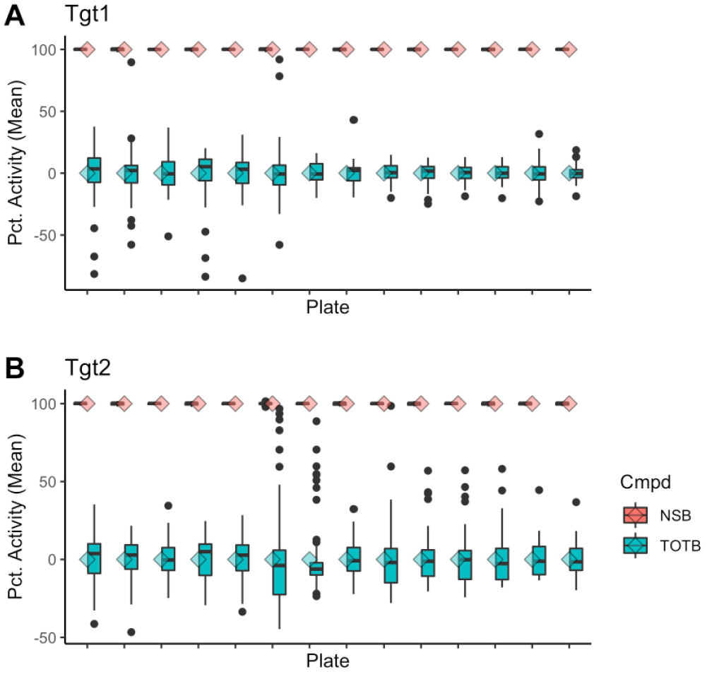
Dose-response plate control. TOTB and NSB control data (N = 64). Plate means are represented as diamonds.

The Z-factor is a common plate statistic and is used to represent the signal/noise of the plate controls. ⁷ Replacing the mean with the median and standard deviation with MAD will yield a robust version of the statistic, Z_robust. Because the Z-factor is unitless, all scaling methods (raw data, mean, median) will provide identical Z-values. Figure 4 shows the results of a paired t test comparing the standard and robust values for the Z-factor per plate. Although most plates show only slight differences, the robust version shows statistically significant improvements in both assays and may represent a better plate quality measurement for these assays.

Figure 4.

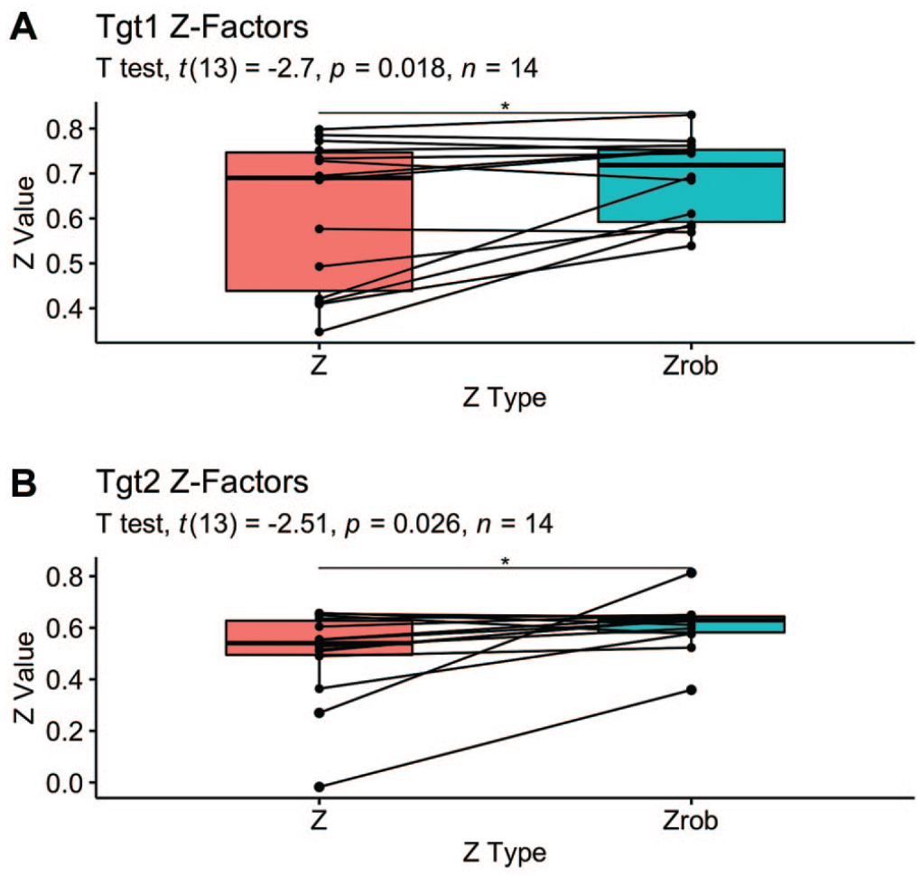
Pairwise comparison of standard and robust Z-factors. Lines link the standard and robust versions of the Z-factor calculated for each plate.

Twelve reference compounds were tested in each assay at 22 different doses with approximately twofold concentration spacing between the doses (CRC). A plate map is included with the Supplemental Materials. These CRCs were replicated four times on each assay plate using randomized well locations. This provides compound test data across the full dynamic range of the assay and allows the comparison of standard and robust data analysis methods, as well as assay reproducibility and performance characteristics.

For the purpose of evaluating nonrobust versus robust summary statistics in a screening context, we took each concentration of each compound to be a different “sample.” The “true” activity for each sample was estimated using the mean or median percentage activity of all 56 wells per sample (four replicates × seven plates × two runs). These means and medians were very similar to each other, given the large sample size. Figure 5A , B , E , F shows the individual well results plotted versus estimated true activity. In this case, the only difference between the nonrobust and robust analysis was how the control well data were summarized per plate, as described in the methods. The most extreme outliers (individual wells) were clearly visible at various levels of percentage activity. The plots also showed that Tgt1 has close to constant variability in the percentage activity scale, whereas Tgt2 had decreasing variability as percentage activity increased. Figure 5C , D , G , H shows the mean or median of the n = 4 replicate wells per plate for each sample plotted versus estimated true activity. In this case, both the control well summaries and the sample replicate summaries were either all nonrobust (means) or all robust (medians). The n = 4 replicate summaries provided a notable reduction in variability relative to the individual well data regardless of analysis method. There were no apparent outliers in the median plots. There were some moderate outliers in the mean plots, which is consistent with the known impact of large outliers on means and not on medians.

Figure 5.

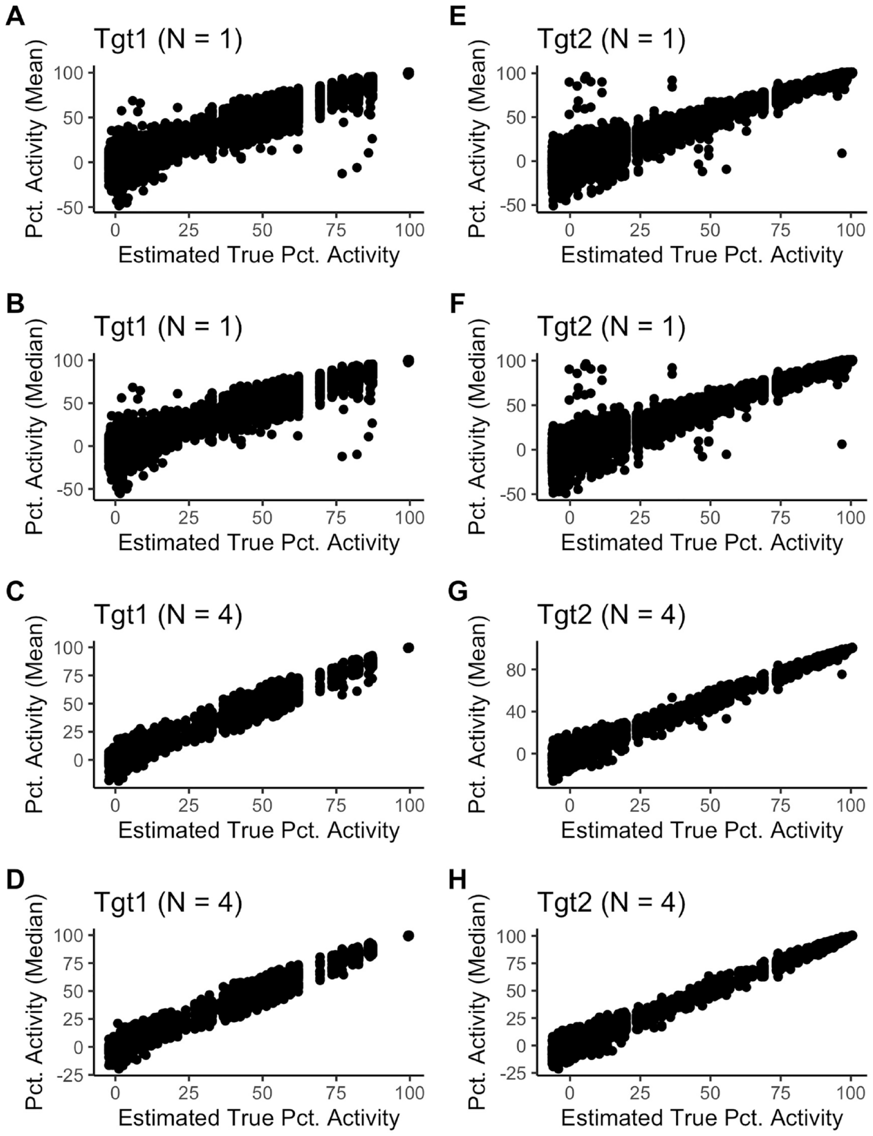
Measured data versus estimated truth.

To assess the impact of using nonrobust versus robust summary statistics on the ability to detect and distinguish active from inactive compounds, we calculated the sensitivity, specificity, positive predictive value (PPV), and negative predictive value (NPV) using the estimated true values per sample as defined above. These statistics were calculated for a range of activity threshold values, from 45% to 75% activity. For a given threshold, T,

• TP = true positive: estimated true activity > T and observed activity > T

• TN = true negative: estimated true activity < T and observed activity < T

• FP = false positive: estimated true activity < T and observed activity > T

• FN = false negative: estimated true activity > T and observed activity < T

• Sensitivity = (No. of true positives)/(No. of true positives + No. of false negatives)

• Specificity = (No. of true negatives)/(No. of true negatives + No. of false positives)

• PPV = (No. of true positives)/(No. of true positives + No. of false positives)

• NPV = (No. of true negatives)/(No. of true negatives + No. of false negatives)

We considered different cutoffs for declaring an active sample, from 45% to 75% activity. Figure 6 shows these results for the individual wells (A, B, E, F) or the n = 4 summaries per plate (C, D, G, H), respectively. In all cases, the results were not noticeably different for specificity, PPV, or NPV; however, the robust approach did provide better sensitivity compared with the nonrobust approach.

Figure 6.

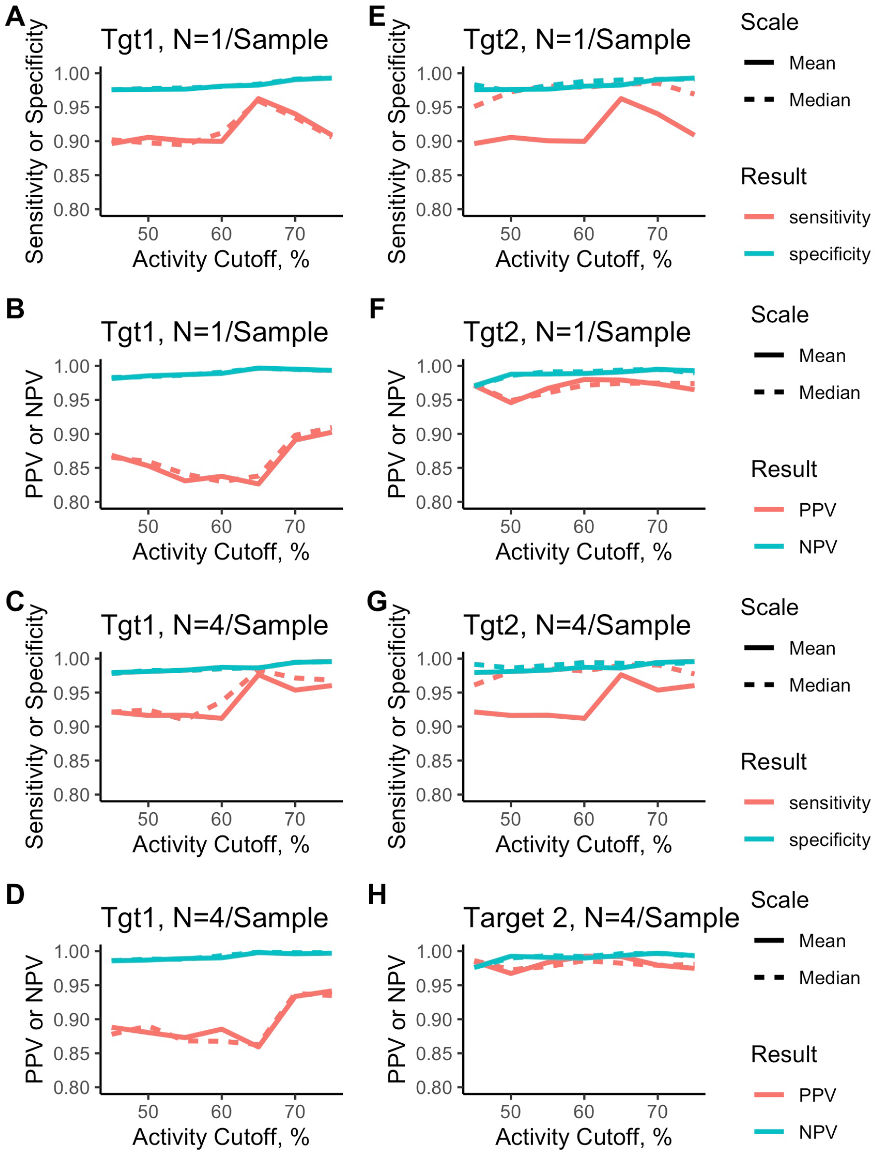
Assay performance measures.

Discussion

Statistical theory suggests that robust methods can slightly underperform or be similar to nonrobust methods when the data conform to the assumptions of a normal distribution with no outliers. The theory also suggests that robust methods perform better when the assumptions are not met. We have considered 2 assays whose data do not conform to those assumptions and shown that the use of robust statistics improved the Z-factors and the sensitivity of both assays; that is, compounds that are active are more likely to be detected as active. The robust and nonrobust methods performed similarly in terms of specificity, PPV, and NPV.

The extreme variability was observed only in the vehicle controls, which define the lower biological range of biological activity. In this case, the primary error that might be observed in screening would be false positives. Similar variability in the active control could also generate false positives.

If a screening lab wanted to use a common approach to the analysis for all their assays, we would recommend the use of robust assay statistics. The robust Z-factors met or exceeded the minimum threshold of 0.4 in the two assays presented here. The unusually large data sets used in this study were designed to illustrate the utility of these methods. In practice, replication rates as low as n = 3 or 4 could be used in assay validation and compound testing to achieve similar benefits.

Supplemental Material

sj-pdf-1-jbx-10.1177_24725552211038379 – Supplemental material for Addressing Unusual Assay Variability with Robust Statistics

Supplemental material, sj-pdf-1-jbx-10.1177_24725552211038379 for Addressing Unusual Assay Variability with Robust Statistics by Jason Haelewyn, Philip W. Iversen and Jeffrey R. Weidner in SLAS Discovery