Sage Journals: Discover world-class research

Abstract

There has been an increase in the use of machine learning and artificial intelligence (AI) for the analysis of image-based cellular screens. The accuracy of these analyses, however, is greatly dependent on the quality of the training sets used for building the machine learning models. We propose that unsupervised exploratory methods should first be applied to the data set to gain a better insight into the quality of the data. This improves the selection and labeling of data for creating training sets before the application of machine learning. We demonstrate this using a high-content genome-wide small interfering RNA screen. We perform an unsupervised exploratory data analysis to facilitate the identification of four robust phenotypes, which we subsequently use as a training set for building a high-quality random forest machine learning model to differentiate four phenotypes with an accuracy of 91.1% and a kappa of 0.85. Our approach enhanced our ability to extract new knowledge from the screen when compared with the use of unsupervised methods alone.

Keywords

artificial intelligence supervised machine learning classification phenotypic profiles

Introduction

After a period in which the pharmaceuticals industry focused greatly on highly reductionist target-based drug discovery, the industry has now in some respects returned to its roots with a much greater emphasis on phenotypic methods.¹ The methods are often employed in more physiologically relevant cell systems such as three-dimensional patient-derived organoids.² The major drawback of reliance on a discovery approach of purely phenotypic drug leads, however, is that the target remains unknown, and the lack of a defined target makes lead optimization more difficult.

High-content screening methods, when combined with multivariate data analytics methods, can provide insight into mechanism of action. This is reflected in the recent interest in Cell Painting, a target agnostic phenotypic profiling method. To be useful for target identification, these methods are often combined with functional genomics.³

Previously, this mostly involved small interfering (siRNA) or small hairpin RNA (shRNA) gene knockdown screens, but as the limitations inherent in these methods, such as off-target effects, became apparent, they fell out of favor.⁴ Recently, there has been more interest in CRISPR-based gene knockout screens, but as with any other new technology, these methods have their own drawbacks that are now becoming apparent.⁵

There are substantial data analytics challenges associated with leveraging the full power of high-content screens. Currently, the most common approach is to use image analysis software to extract numeric descriptors of the cellular phenotype at either the well or object (cell or organoid) level. This need can generally be met with commercial image analysis platforms that are delivered with automated high-content imagers or the open-source CellProfiler platform.⁶ Other options that require more specialist expertise include Image J⁷ and image analysis functionality that is available in the KNIME data pipelining platform.⁸

The mining of the resultant numeric data sets has been more problematic. PerkinElmer provides an adapter for the Tibco Spotfire data visualization tool called High Content Profiler. Genedata support high content in their Screener platform. In this study, the data are mined using the HC StratoMineR platform.⁹ We have previously shown how this platform can be used to mine high-content data sets using an exploratory, unsupervised data analytics workflow, in which data reduction followed by the calculation of a multidimensional distance score that allows for the detection of phenotypic outliers. These outliers could then be subjected to hierarchical clustering to identify groups with similar phenotypes.^9–11

One drawback of an unsupervised approach is that it is difficult to connect the structure within the clustering with the underlying biology. Here, we seek to better connect the biologist with the reasons why certain outliers are clustering together.

An alternative approach to the unsupervised method^9–11 would be to use supervised machine learning approaches.¹² These are popularly referred to as artificial intelligence (AI). A training set is used to build a multiclass model that can subsequently be used to classify reagents in a high-content screen according to similarity to one or more interesting phenotypes.

A number of studies in the area of high-content screening have applied machine learning to high-resolution data. Neumann et al.¹³ took 190,000 time-lapse movies from 19 million cell divisions. Approximately 200 features were extracted using segmentation, and 3000 nuclei were manually annotated. The set was used to train a support vector machine (SVM) classifier with an accuracy of 87%. The 1.9 billion nuclei were classified into 1 of 16 morphological classes. Phenotypic profiles were used to classify deviations from control groups and identify relevant changes. Genome-wide scores were used to flag mitotic hits.

Fuchs et al.¹⁴ conducted a siRNA screen in HeLa cells to generate automated high-content screening images stained for DNA, tubulin, and actin. The cell body and nuclei were segmented, and features were extracted from all three channels. Finally, cells were classified using an SVM model based on eight cellular phenotype classes. This was built on a training set of 1740 cells. The measured accuracy ranged from 96.9% to 100%.

Ljosa et al.¹⁵ used CellProfiler to generate 453 features for 2.2 million cells from MCF-7 breast cancer cells treated with 113 different compounds at eight concentrations. Cell data were standardized and normalized prior to analysis. Mean values, Kolmogorov-Smirnov statistics, SVM, and factor analysis were used to calculate profile values for each treatment. Then, a mechanism of action score was generated from the calculated statistics.

Advanced Cell Classifier and the Analyst module of CellProfiler allow for the annotation of machine learning classes by directly selecting cell images.^16,17 No matter what populations are chosen, the quality of the analysis is heavily dependent on the quality of the training set used. We hypothesized that the unsupervised data analytics pathway^9–11 would be useful for the generation of a high-quality training set that could then be successfully used to build an effective machine learning model. In this study, the approach of unsupervised analysis followed by a supervised analysis is carried out on a data set that was previously analyzed.^9,18 We show that the combination of unsupervised and supervised data analytics methods has the potential to enhance the ability to identify new knowledge in functional genomics screens.

Materials and Methods

Wet-Lab Protocol and Data Set

The data set used in this study is a genome-wide high-content siRNA screen that was performed to identify novel regulators in mitosis. In short, a Dharmacon (Lafayette, CO) genome-wide ON-TARGETplus siRNA SMARTpool library was transfected in HeLa cells in 384-well microplates (1500 cells per well). After fixation, the cells were stained with diamidino-2-phenylindole (DAPI) after siRNA knockdown for the identification of the nucleus and an antibody against phosphorylated histone H3 to identify cells in mitosis.

Images were acquired using a Thermo (Waltham, MA) Array Scan VTi, and numeric features for each cell were extracted using the Cellomics Target Activation/Morphology Explorer image analysis software. The methods used in this screen are described in much greater detail elsewhere.^9,18 The data set contains ~46 million records, and each record represents a single cell, consisting of 74 features.^9,18 To carry out the data analysis, the data were exported to flat files, one per microplate. The data were available in two resolutions: low (well averages, each record is a well) and high (object level, each record is a cell), and in two cell lines.

Data Preprocessing

Preprocessing data is a very tedious but important part of a data analysis process.^9,19,20 First, data are divided into meta features (information about the data) and analytical features (used for data analysis). Examples of analytical features are intensity, area, shape, and texture features on various channels (Thermo Scientific, 2010; retrieved from http://www.med.cam.ac.uk/wp-content/uploads/2016/02/MorphologyExplorer_V4_LC06170800.pdf). Features with a standard deviation of 0 or containing ≥95% missing data are omitted. Those with a correlation coefficient ≥0.99 are inspected for missing data, and only the feature with the lowest number of missing data points is retained.

An additional feature selection is then performed by omitting features containing an equal uniform distribution across the different classes. Features are then normalized on a plate-by-plate basis by dividing each feature by the median of the negative control (scrambled siRNA). The z-distribution of the skewness is inspected for significance (p < 0.001). Here, the Kolmogorov-Smirnov and Shapiro-Wilk tests are too sensitive.^21–23 Features are log transformed in cases of positive skewness and transformed using a square root in cases of negative skewness. Finally, features are scaled using a robust z-score.²⁴

A significant missing completely at random (MCAR) outcome results in case-wise deletion of missing data, whereas an insignificant MCAR outcome is handled by imputation methods (e.g., regression, random forest [RF], or predictive mean matching).^25,26 The method described by Young et al.,¹⁰ Omta et al.,⁹ and Caicedo et al.¹¹ focuses on the numeric data analysis after preprocessing, as described above to identify hits. The number of features that are left over after preprocessing can subsequently be included for carrying out further analysis (i.e., exploratory, descriptive, or predictive analysis). All of the analysis results were generated using R and HC StratoMineR.^9,27 All data analyses were carried out on an AWS EC2 r5.xlarge with an Intel Xeon Platinum 8000 series with four cores and 32 GB of RAM. This hardware was used because it can be compared with a standard modern laptop.

Results

In this study, the siRNA data set was reanalyzed with a similar strategy to that used in the original study,^9,18 followed by a supervised machine learning approach. The complete data analysis workflow in this article was carried out in four stages: stage A (exploratory data analysis) is an unsupervised approach ( Fig. 1A ), stage B (annotation) involves the annotation of the data in preparation for stage C ( Fig. 1B ), stage C (predictive data analysis) is a supervised machine learning stage ( Fig. 1C ), and in stage D (evaluation), the results of stage C are evaluated ( Fig. 1D ). The data set used in these stages contains 41 useful features that were extracted from the DAPI and pS10-H3 channels.

Figure 1.

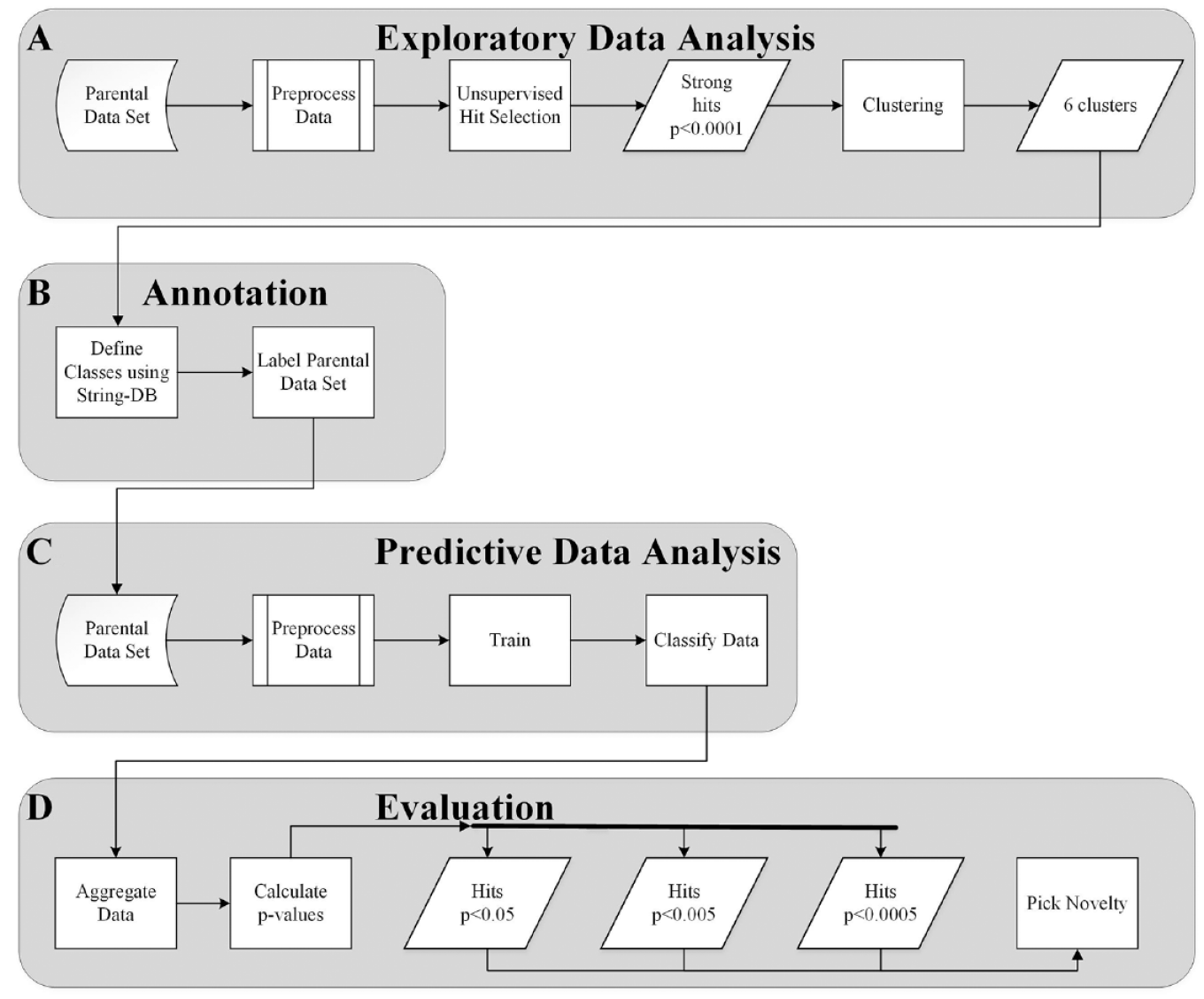
Process of combining unsupervised with supervised analysis. (A) Describes the exploratory data analysis using well-resolution data carried out in an unsupervised fashion. (B) Describes the annotation process in which classes are labeled using the results of A and using a GO-term analysis from String-DB. (C) Describes the predictive analysis stage. A supervised machine learning model is trained based on the data that was annotated in stage B. (D) Describes the aggregation of the results and the evaluation of the four hit lists that are generated.

Stage A: Exploratory Data Analysis

The first stage in the data analysis workflow is an exploratory data analysis stage or unsupervised approach ( Fig. 1A ) using well-level resolution data, which was carried out as described in Omta et al.⁹ The data in this stage contains only ~47,000 records per cell line (two cell lines). After preprocessing, data reduction was carried out using common factor analysis. Common factor analysis generated five common factors that were then used to calculate a Euclidean distance score from the median of the negative controls. In addition, p values were calculated and are based on the negative controls and corrected with the false discovery rate (FDR) to avoid type II errors. For each screened siRNA pool, the difference between the distance scores from the parental and EIC cell lines was calculated. Those that came from wells that had a p value <0.05 in the parental cell line were chosen as hits. The genes targeted by these 154 siRNA pools were analyzed in String-DB.²⁸ As we have seen previously in our analysis, the hit list was enriched for genes involved in mitosis, but also ribosomal genes, genes related to proteasomal degradation, and splicing genes. In this and subsequent String-DB analyses, we followed four Biological Process GO terms: (1) GO:1903047 or mitotic cell cycle process, which we refer to as “mitosis” (red dots in Fig. 2 ); (2) GO:0006413 or translational initiation, referred to as “ribosome” (green dots in Fig. 2 ); (3) GO:0000398 mRNA splicing, via spliceosome, referred to as “splicing” (purple dots in Fig. 2 ); and (4) GO:0016579 protein deubiquitination, referred to as “proteasome” (yellow dots in Fig. 2 ). Within our 154 hits, it was clear that mitosis genes were poorly enriched (15 genes, FDR = 0.001) compared with splicing (30 genes, FDR = 7.21E-22), proteasome (16, FDR = 3.92E-08), and ribosome (25 genes, FDR = 1.12E-22). This would suggest that looking for novel mitosis genes in the unconnected or gray nodes would be far more likely to deliver genes involved in one of the other processes (see Fig. 2 ).

Figure 2.

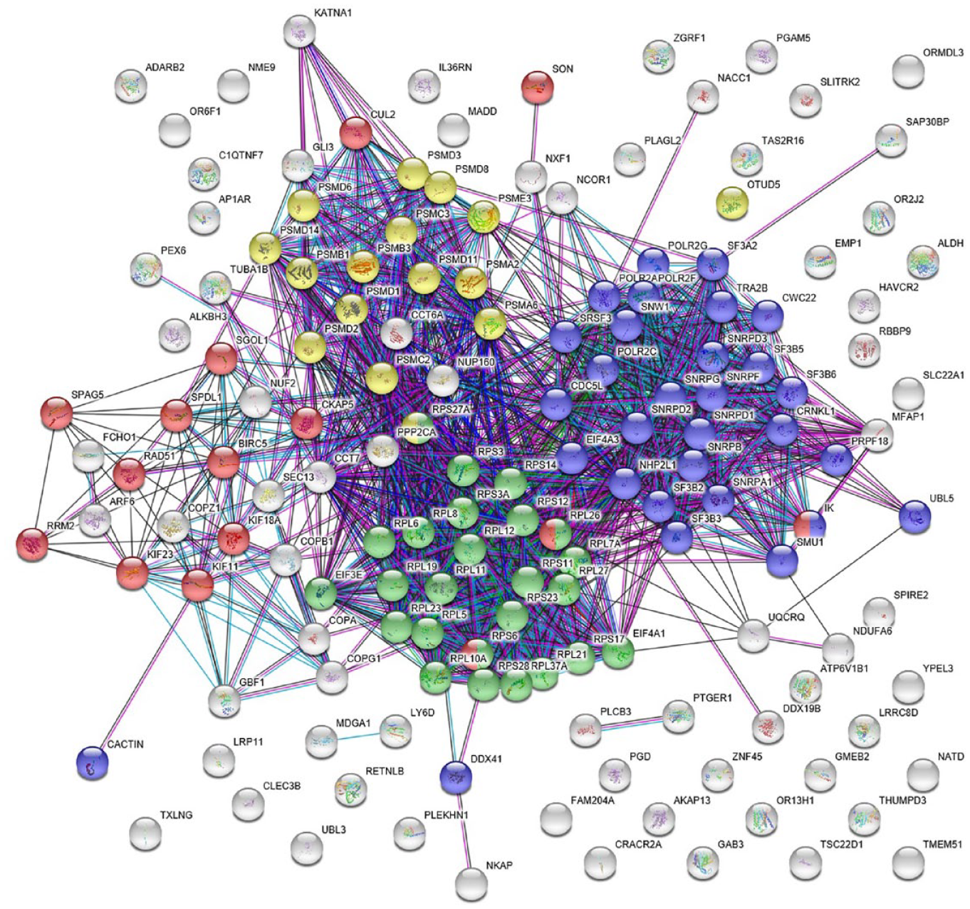
The interaction of a set of 154 genes that resulted from the analysis of comparing the parental cell line to the EIC cell line was visualized using String-DB. Four pathways in this set were found to be significantly enriched: (1) mitotic cell-cycle process (Mitosis, GO:1903047; 15/154 genes, false discovery rate [FDR] = 0.001) visualized in red; (2) translational initiation (Ribosome, GO:0006413; 25/154 genes, FDR = 1.12E-22) visualized in green; (3) mRNA splicing, via spliceosome (Splicing, GO:0000398; 30/154 genes, FDR = 7.21E-22) visualized in purple; and (4) protein deubiquitination (Proteasome, GO:0016579; 16/154 genes, FDR = 3.92E-08) visualized in yellow. Gray items are unknown to the ontology.

In a previous study, hierarchical clustering was used to identify groups of genes that were highly enriched for mitotic cell-cycle genes.⁹ The addition of supervised machine learning functionality now provided the opportunity to use a new strategy that could combine the unsupervised and supervised data analytics approaches to address the problem.

A higher-resolution parental data set was available at cell resolution as opposed to well-averaged data. We used the distance-based unsupervised method to identify 344 very strong hits. siRNAs that showed a significant difference (p < 0.0001) from the negative control (scrambled siRNA) using a multiparametric distance score^9–11 (see Fig. 1A ) were subjected to hierarchical clustering in combination with K-means clustering, in which six clusters were generated (see Fig. 1A ). Analysis of these in String-DB highlighted four clusters that were highly enriched for mitosis, splicing, proteasome, & ribosome genes (see Fig. 3 ). From the hierarchical cluster analysis and K-means clustering, each cluster was submitted to String-DB separately (see Supplementary Data S1, S2, S3, and S4). Cluster 2 (Supplementary Data S2) was clearly most enriched for mitosis genes (14 of 48 genes, FDR = 4.39E-09) and cluster 5 (Supplementary Data S4) for ribosomal genes (30 of 95 genes, FDR = 9.25E-36). Interestingly, the splicing and proteasome genes proved more difficult to separate but both were distributed across cluster 3 (Supplementary Data S3; splicing, 11 of 69 genes, FDR = 3.37E-12; proteasome, 11 of 69, FDR = 0.0011; and mitosis, 13 of 69 genes, FDR = 1.08E-05). Cluster 1 (Supplementary Data S1; splicing, 15 of 55, FDR = 1.76E-12; proteasome, 7 of 55 genes, FDR = 0.00089). It was notable that cluster 1 was centered around ubiquitin-C (see Supplementary Data S1), whereas cluster 3 was centered around ubiquitin-B (see Supplementary Data S3). Cluster 1 also had significant enrichment for mitotic genes (7 of 55, FDR = 0.0233; see Supplementary Data S1). This information was taken from the String-DB Homo Sapiens Process ontology. The enrichment and annotation were verified using Gorilla²⁹ and confirms our findings with an FDR of 4.64E-02 of mitosis in cluster 2, an FDR of 1.22E-5 of ribosome in cluster 5, and an FDR of 4.99E-02 of splicing in cluster 1.

Figure 3.

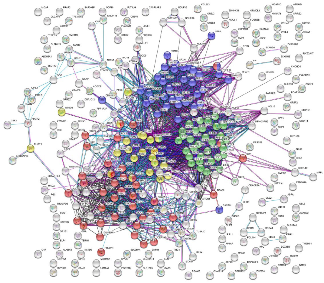
The interaction of a set of 344 resulting genes from the unsupervised analysis of the parental cell line was visualized using String-DB. Four pathways in this set were found to be significantly enriched: (1) mitotic cell-cycle process (mitosis, GO:1903047), visualized in red; (2) translational initiation (ribosome, GO:0006413), visualized in green; (3) mRNA splicing, via spliceosome (splicing, GO:0000398), visualized in purple; and (4) protein deubiquitination (proteasome, GO:0016579), visualized in yellow. Gray items are unknown to the ontology.

Stage B: Annotation

We randomly chose a total of 52 genes (~124,000 cells) from the hit list containing 344 genes that was generated in stage A to label the data and to create a training set for training a four-class classifier model at single-cell level in stage C (see Fig. 1C ). The resulting GO-Terms from String-DB were used to annotate the siRNAs that showed significant involvement in the four identified pathways in stage A (see Fig. 1A ). We chose 15 mitosis genes (GO:1903047) from cluster 2 for the mitotic class (~36,000 cells) and 13 ribosome genes (GO:0006413) from cluster 5 for the ribosome class (~31,000 cells). Because both splicing (GO:0000398) and proteasome (GO:0016579) genes are across clusters 1 and 3, we decided to build a ProteaSplice class using 24 proteasome and splicing genes (~57,000 cells). The fourth class is a rest class and is introduced with the ability to capture cells belonging to neither of the three pathway classes. The rest class is a scrambled siRNA and labeled as NEGATIVE, which was originally already present in the data set.

Stage C: Predictive Data Analysis

Using the results of the unsupervised approach to label the object-level resolution data with three additional training classes as described in stage B is then followed by a supervised machine learning approach (see Fig. 1C ). In the predictive data analysis or supervised approach (stage C), data at the object level is used and contains ~57 million records. Instead of calculating a distance score, as previously has been done with well resolution data^9–11 a classification algorithm is used in stage C, using data at the object level.

To explore the possible classification and feature-driven approaches, a preliminary analysis was conducted including three classification algorithms. In addition, principal component analysis (PCA), independent component analysis (ICA), or the original feature set was used for building classification models (see the column labeled “Features/PCA/ICA” in Table 1 ). Both PCA and ICA are methods used to reduce the dimensionality. These methods support the reduction of redundancy, bias, and required computational power and attempt to avoid the curse of dimensionality.³⁰ The results of the preliminary analysis can be seen in Table 1.

Table 1.

Exploration of Algorithms and the Data Feature Space.

Scenario	Classification Algorithm	Features/PCA/ICA	Accuracy, %	Kappa	Time, s
1	Random forest (mtry = 20)	Features	96.01	0.917	106.616
2	Random forest (mtry = 4)	PCA	86.44	0.729	35.302
3	Random Forest (mtry = 4)	ICA	85.91	0.7183	36.219
4	Support vector machine (sigma = 0.03768469, C = 43.53546)	Features	96.02	0.920	1517.326
5	Support vector machine (sigma = 0.0657829, C = 477.636)	PCA	86.82	0.736	3460.237
6	Support vector machine (sigma = 0.1616871, C = 43.53546)	ICA	86.63	0.7327	2491.188
7	Neural networks (size = 20, decay = 1.044708e-03)	Features	96.57	0.931	96.339
8	Neural networks (size = 20, decay = 1.044708e-03)	PCA	86.43	0.729	49.987
9	Neural networks (size = 20, decay = 1.044708e-03)	ICA	86.03	0.7207	53.248

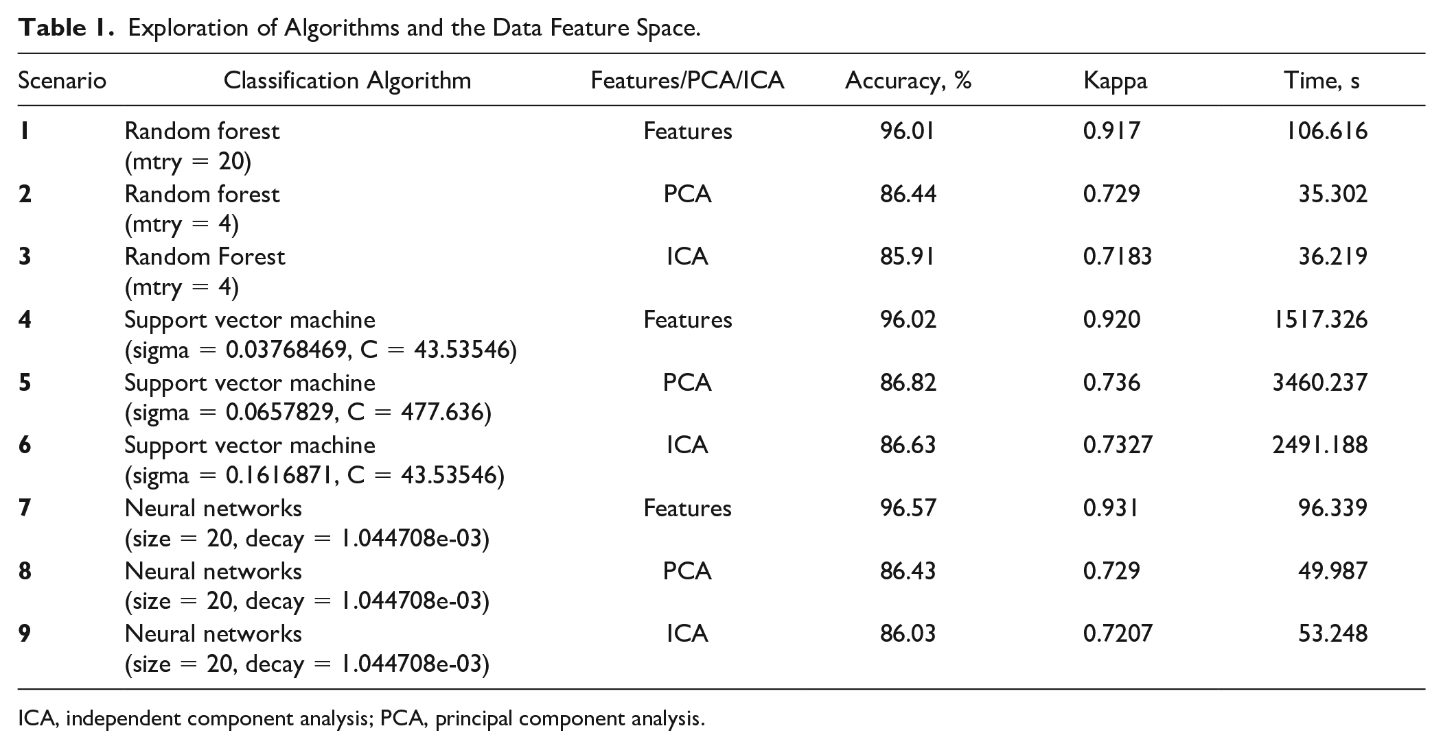
ICA, independent component analysis; PCA, principal component analysis.

The features are simply the original features available in the data set that were treated as described in the Data Preprocessing section. The PCA approach implies the same preprocessing approach and the creation of seven principal components (based on the elbow method) using a generalized least-squares approach.³¹ The ICA approach also implies the same preprocessing treatment and the creation of seven components using a nonlinear method.³² For this preliminary analysis, binary classification models were trained³³ using built-in NEGATIVE and POSITIVE controls to explore the options of the original feature space or dimensionality reduction in combination with three classification algorithms.

In all nine scenarios, 50,000 records were randomly sampled with replacement of the total set of ~325,000 records³⁴ of data containing the label NEGATIVE or POSITIVE. The 50,000 records were then split into an 80% train set and a 20% test set. For the optimization of the hyperparameters, a fourfold cross-validation was applied to the train set.³⁵

A random search grid was created to find the optimal hyperparameter settings for all nine scenarios³⁶ (see Table 1 ). For RFs,³⁷ trees were constantly kept at 128 trees,³⁸ and the hyperparameter mtry was tuned (see Table 1 ). For SVM,³⁹ a radial kernel was chosen,⁴⁰ and the hyperparameters sigma and C were tuned to optimize the performance of SVM. For neural networks,⁴¹ an architecture of one layer was used. The hyperparameter size and decay were tuned. The hyperparameter size implies the number of nodes in the hidden layer. The hyperparameter decay implies the penalty for the size of the weights. The output of tuning the neural network hyperparameters size and decay was the same for all three cases (features, PCA, and ICA).

The hyperparameters for SVM and neural network are hard to tune and to understand compared with the hyperparameter of RF. SVM performs well but is very slow. Our final decision is RF because of the ease of use (minimal hyperparameter tuning), the speed of the algorithm (see Table 1 ), and the relative low chance of overfitting.⁴² We chose single features over a dimensionality reduction method because RF builds trees based on a random set of features (mtry). RF is not very sensitive to the number of random features (mtry), the total number of features, and the tree size with respect to overfitting.⁴² This work was carried out in R using the packages nnet, e1071, and randomForest.

For the classification and identification of our siRNAs and targets, a supervised multiclass machine learning model using RF⁴³ was built based on the four classes described in stage B. Each single cell can be classified into one of these classes according the model using the feature space of the data set. Stratified data sampling was carried out because of variation in class size (see stage B).

The multinomial RF model was applied in classification mode and trained using 128 trees.³⁸ The labeled data, containing ~430,000 cells was split into 80% training and 20% for testing.⁴⁴ The model was trained using ~345,000 data points in fourfold cross-validation and showed a substantial Kappa agreement score, which corrected for agreement expected by chance,⁴⁵ between the observed and predicted classes of 0.8517 and an accuracy of 91.1%.^45,46 A random search grid was created to tune the RF model to find the ideal hyperparameter setting. The hyperparameter setting mtry =10 was finally found to be the best option.

The Kappa score can be explicitly important to data sets with imbalanced or skewed classes (see stage B). Table 2 shows the resulting confusion matrix of the classification model. A confusion matrix allows for an indication of the model’s accuracy in classifying the test data set. Each row represents the actual class of the cells, and each column represents the predicted class of the cells. Each number represents the percentage of cells predicted within the grid. The diagonal in bold shows the percentages that are predicted correctly.

Table 2.

Cellular Resolution Multiclass Classification.^a

		Predicted Class (Cellular Resolution)
		Mitosis	NEGATIVE	ProteaSplice	Ribosome	Total
Actual class (cellular resolution)	Mitosis	92.65% (10,427)	4.18% (470)	2.11% (238)	1.06% (119)	100% (11,254)
	NEGATIVE	0.87%(437)	92.50% (46,729)	4.72%(2384)	1.92%(969)	100%(50,519)
	ProteaSplice	1.09%(178)	11.50%(1877)	86.06% (14,047)	1.35%(220)	100%(16,322)
	Ribosome	0.68%(56)	7.21%(597)	1.73%(143)	90.38% (7481)	100%(8277)

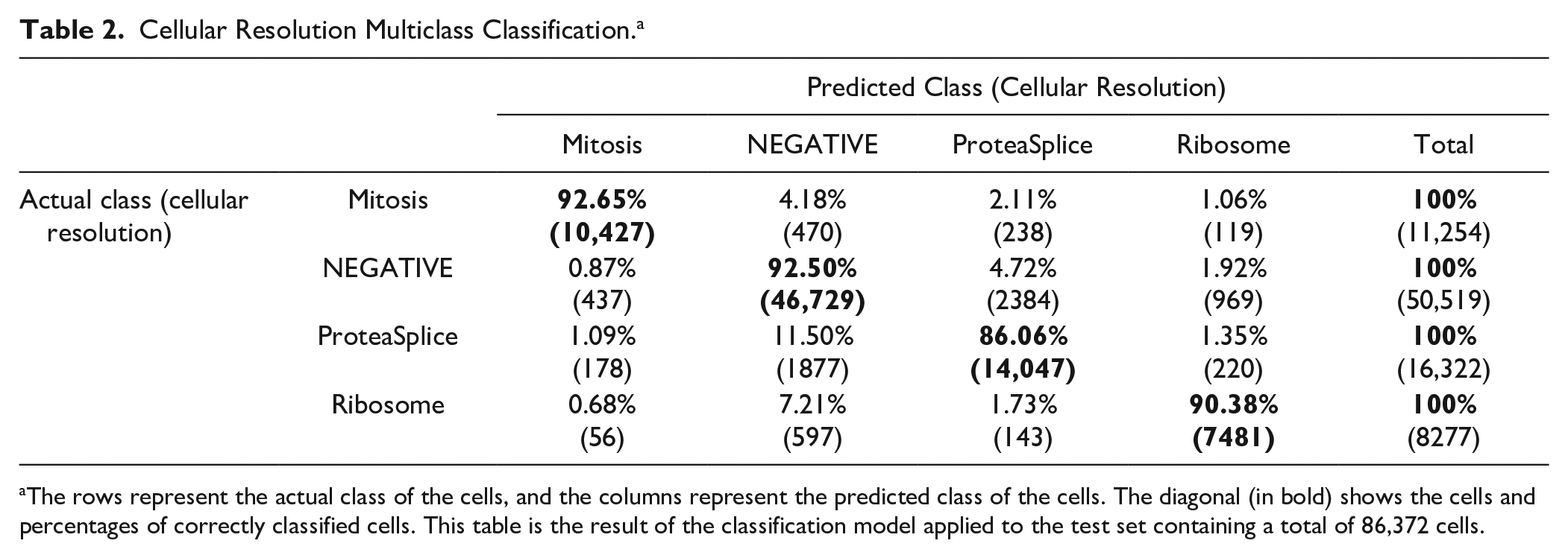
The rows represent the actual class of the cells, and the columns represent the predicted class of the cells. The diagonal (in bold) shows the cells and percentages of correctly classified cells. This table is the result of the classification model applied to the test set containing a total of 86,372 cells.

Stage D: Evaluation

We applied this model to the entire parental data set. Each cell in every well across the data set was classified into one of the four classes. This information was then aggregated using medians and standard errors as an estimator per well to generate the probabilities of each well being a member of the four classes. We ranked all the wells according to the probability that they were in the mitotic class and generated four hit lists based on P-value cutoffs of 0.05, 0.005, 0.0005, and 0.00005 with 16%, 23%, 29%, and 38% of mitosis genes, respectively (see Fig. 4A ). Figure 4B demonstrates the same data but in absolute numbers.

Figure 4.

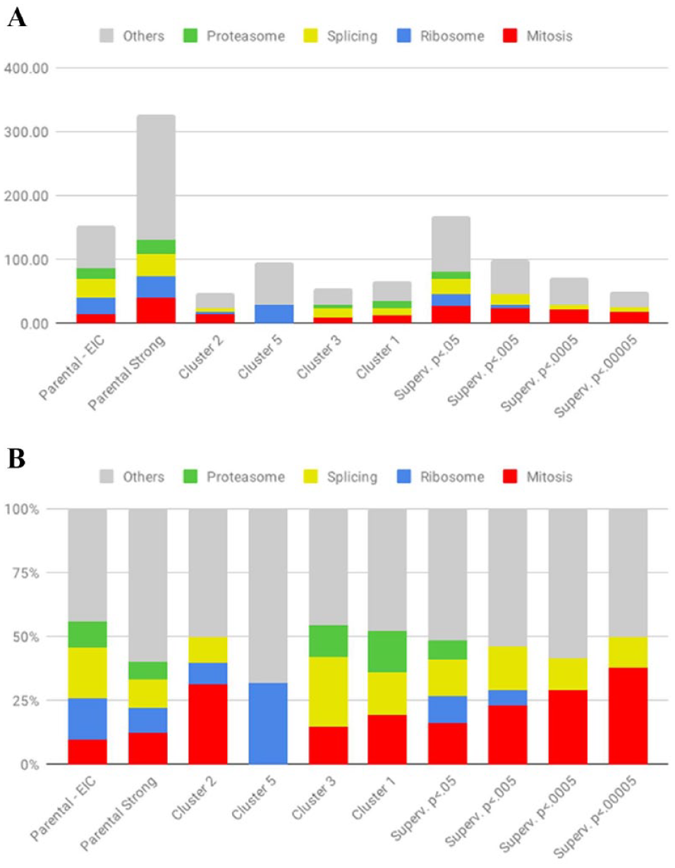
Results classification.

To determine the likelihood that our approach would make it easier to identify novel regulators of mitosis, we carried out a simple search in PubMed for [Gene Name] AND Mitosis for the genes in the p < 0.0005 list, not assigned to any of our key GO groups. Four genes, FAM110,⁴⁷ Rec114,⁴⁸ UBR5,⁴⁹ and NKAP,⁵⁰ were found to have been recently reported to be involved in mitosis or meiosis.

Discussion

Our study has demonstrated how the combination of unsupervised and supervised machine learning can greatly enhance the efficiency with which new knowledge can be extracted from functional genomics screens. Our original analysis, relying solely on unsupervised methods, resulted in a hitlist that was overwhelmed with hits that were of little interest because they were already known to be involved in the core machinery of protein translation, degradation, and RNA splicing. It could well have been that interesting hits with novel mechanisms of action could have been found in this, but these would have been difficult to identify.

The unsupervised analysis did prove to be very useful, however, as identifying hits using a multiclass RF model allowed for the generation of hit lists that were far more heavily enriched in genes that were centrally involved in mitosis.

In this case, this approach could potentially have been used to generate more information from a genome-wide screen that generated only a single publication on three genes that were already known to be involved in mitotic spindle assembly. Confirming that there are novel regulators of mitosis in the supervised machine learning hit lists is unfortunately beyond the scope of this study, but we believe that our approach provides biologists the opportunity to be able to deal better with the challenges of validating and characterizing hits from functional genomics screens.

Results of unsupervised machine learning can be used as input for rich data visualizations. In-depth data exploration using these visualizations allows for identifying patterns, systematic errors, false-positives, and outliers to add labels to subpopulations and add value to the data set.⁵¹ These manual annotations are invaluable for training a supervised machine learning model. The supervised model can be trained using the annotations and can be applied to classify new (unseen) data.

The classification result contains a probability score for each class in each record. Each probability score represents the likelihood that a record belongs to a class. The sum of the probabilities of the classes for each record is equal to 1. The set of probabilities represents a matrix pm and contains as many records as the classified data set. The number of columns of matrix pm is equal to the number of classes that are included in the supervised classification model.

Supplementary Data S5 demonstrates a hypothetical example of the output of a three-class classification model in a probability matrix (pm). The matrix pm is visualized using a heatmap and clustered using an unsupervised method to organize the data according to similarity. When a cluster contains records with equally distributed probabilities among the classes (~0.33), we hypothesize that the cluster belongs to a fourth class. This approach of combining unsupervised and supervised machine learning can potentially be used to generate new classes and identify new phenotypes.

One major challenge in phenotypic screening is how to gain insight into what distinguishes different phenotypes. Using the unsupervised fashion, we can create groups of phenotypes using a combination of hierarchical clustering and common factor analysis or PCA profiles. In extreme cases, looking at the images is enough to be able to define what is different (e.g., a cluster of toxic reagents). In many cases, however, the differences are subtle and hard to define. Tracking back through principal components to identify extracted features that are contributing to phenotypic differences is also not efficient.

However, through the feature importance plot from a supervised machine learning model, one can observe what the key differentiating features are for a set of classes (see Supplementary Data S6). This provides an immediate insight into the biology, especially in a two-class model in which one of the classes is based on the negative controls. For screens in which the goal is to identify reagents that give one phenotype, this would allow a screener to simplify feature extraction, by limiting it to the critical features and reducing the abundance of redundant features that can be extracted nowadays. This could be especially useful for screens based on the Cell Painting method.³

One possible improvement to the proposed method in this article would be to allow users to build supervised machine learning models on subpopulations of cells within wells and not just on all-cells-in-well populations. In commercial platforms, this is currently possible at the image level, for example, in PE Columbus, by clicking on individual cells and assigning them to individual classes. The recently introduced Phenoglyphs functionality in GE’s IN Carta platform allows a user to define the classes in a more iterative fashion. The Classifier function in the open-source CellProfiler Analyst¹⁷ offers similar functionality to the open-source Advanced Cell Classifier¹⁶ platform.

Machine learning methods have long been applied in the analysis to high-content data sets, but this has almost exclusively been in a post hoc analysis, by data scientists writing project-specific scripts. The availability of AI functionality in the StratoMineR platform and the other tools described above gives the screener the ability to leverage the power of AI, but it is critical that the screener can validate the quality of the generated model.

The use of convolutional neural networks to classify high-content images directly can be done using deep learning. Deep learning allows for an alternative approach without the intermediate step of conducting feature extraction, and it is attracting much attention.⁵² The success of these approaches, however, will also highly depend on the quality of the training sets used and the quantity of available data in each training class. We believe that this will require an analogous method to the one we describe here.

Supplemental Material

OmtaSuppplDataR2 – Supplemental material for Combining Supervised and Unsupervised Machine Learning Methods for Phenotypic Functional Genomics Screening

Supplemental material, OmtaSuppplDataR2 for Combining Supervised and Unsupervised Machine Learning Methods for Phenotypic Functional Genomics Screening by Wienand A. Omta, Roy G. van Heesbeen, Ian Shen, Jacob de Nobel, Desmond Robers, Lieke M. van der Velden, René H. Medema, Arno P. J. M. Siebes, Ad J. Feelders, Sjaak Brinkkemper, Judith S. Klumperman, Marco René Spruit, Matthieu J. S. Brinkhuis and David A. Egan in SLAS Discovery

Footnotes

Acknowledgements

We would like to thank René Eijkemans and Wigard Kloosterman for the useful discussions in machine learning and cell biology.

Supplemental material is available online with this article.

Declaration of Conflicting Interests

The authors declared the following potential conflicts of interest with respect to the research, authorship, and/or publication of this article: W.A.O. and D.A.E. are founders and shareholders of Core Life Analytics, a company that develops and markets data analytics software including H.C. StratoMineR, which has been used in this work.

Funding

The authors received no financial support for the research, authorship, and/or publication of this article.

ORCID iDs

Marco René Spruit

Matthieu J. S. Brinkhuis

References

Moffat

J. G.

Vincent

Lee

J. A.

; et al. Opportunities and Challenges in Phenotypic Drug Discovery: An Industry Perspective. Nat. Rev. Drug Discov. 2017, 16, 531.

Yang

; et al. Tumor Organoids: From Inception to Future in Cancer Research. Cancer Lett. 2019, 454, 120–133.

Bray

M. A.

Singh

Han

; et al. Cell Painting, a High-Content Image-Based Assay for Morphological Profiling Using Multiplexed Fluorescent Dyes. Nat. Protoc. 2016, 11, 1757.

Seok

Lee

Jang

E. S.

; et al. Evaluation and Control of miRNA-Like Off-Target Repression for RNA Interference. Cell. Mol. Life Sci. 2018, 75, 797–814.

Munoz

D. M.

Cassiani

P. J.

; et al. CRISPR Screens Provide a Comprehensive Assessment of Cancer Vulnerabilities but Generate False-Positive Hits for Highly Amplified Genomic Regions. Cancer Discov. 2016, 6, 900–913.

Carpenter

A. E.

Jones

T. R.

Lamprecht

M. R.

; et al. CellProfiler: Image Analysis Software for Identifying and Quantifying Cell Phenotypes. Genome Biol. 2006, 7, R100.

Rueden

C. T.

Schindelin

Hiner

M. C.

; et al. ImageJ2: ImageJ for the Next Generation of Scientific Image Data. BMC Bioinform. 2017, 18, 529.

Dietz

Berthold

M. R.

KNIME for Open-Source Bioimage Analysis: A Tutorial. In Focus on Bio-Image Informatics; De Vos

W. H.

Munck

Timmermans

J.-P.

, Eds.; Springer: Cham, 2016, pp. 179–197.

Omta

W. A.

van Heesbeen

R. G.

Pagliero

R. J.

; et al. HC StratoMineR: A Web-Based Tool for the Rapid Analysis of High-Content Datasets. Assay Drug Dev. Technol. 2016, 14, 439–452.

10.

Young

D. W.

Bender

Hoyt

; et al. Integrating High-Content Screening and Ligand-Target Prediction to Identify Mechanism of Action. Nat. Chem. Biol. 2008, 4, 59–68.

11.

Caicedo

J. C.

Cooper

Heigwer

; et al. Data-Analysis Strategies for Image-Based Cell Profiling. Nat. Methods 2017, 14, 849–863.

12.

Scheeder

Heigwer

Boutros

Machine Learning and Image-Based Profiling in Drug Discovery. Curr. Opin. Syst. Biol. 2018, 10, 43–52.

13.

Neumann

Walter

Hériché

J. K.

; et al. Phenotypic Profiling of the Human Genome by Time-Lapse Microscopy Reveals Cell Division Genes. Nature 2010, 464, 721–727.

14.

Fuchs

Pau

Kranz

; et al. Clustering Phenotype Populations by Genome-Wide RNAi and Multiparametric Imaging. Mol. Syst. Biol. 2010, 6, 370.

15.

Ljosa

Caie

P. D.

Ter Horst

; et al. Comparison of Methods for Image-Based Profiling of Cellular Morphological Responses to Small-Molecule Treatment. J. Biomol. Screen. 2013, 18, 1321–1329.

16.

Piccinini

Balassa

Szkalisity

; et al. Advanced Cell Classifier: User-Friendly Machine-Learning-Based Software for Discovering Phenotypes in High-Content Imaging Data. Cell Syst. 2017, 4, 651–655.

17.

Dao

Fraser

A. N.

Hung

; et al. CellProfiler Analyst: Interactive Data Exploration, Analysis and Classification of Large Biological Image Sets. Bioinformatics 2016, 32, 3210–3212.

18.

van Heesbeen

R. G.

Raaijmakers

J. A.

Tanenbaum

M. E.

; et al. Aurora A, MCAK, and Kif18b Promote Eg5-Independent Spindle Formation. Chromosoma 2017, 126, 473–486.

19.

Wickham

Tidy Data. J. Stat. Softw. 2014, 59, 1–23.

20.

Omta

W. A.

van Heesbeen

R. G.

Shen

; et al. PurifyR: An R Package for Highly Automated, Reproducible Variable Extraction and Standardization. Syst. Med. 2020, 3, 1–7.

21.

Royston

Algorithm

181: The W Test for Normality. Appl. Stat. 1982, 31, 176–180.

22.

Royston

An Extension of Shapiro and Wilk’s W Test for Normality to Large Samples. Appl. Stat. 1982, 31, 115–124.

23.

Marsaglia

Tsang

W. W.

Wang

Evaluating Kolmogorov’s Distribution. J. Stat. Softw. 2003, 8–18.

24.

Birmingham

Selfors

L. M.

Forster

; et al. Statistical Methods for Analysis of High-Throughput RNA Interference Screens. Nat. Methods 2009, 6, 569–575.

25.

Buuren

S. V.

Groothuis-Oudshoorn

mice: Multivariate Imputation by Chained Equations in R. J. Stat. Softw. 2010, 45, 1–68.

26.

Little

R. J.

A Test of Missing Completely at Random for Multivariate Data with Missing Values. J. Am. Stat. Assoc. 1988, 83, 1198–1202.

27.

Ripley

B. D.

The R Project in Statistical Computing. MSOR Connections. 2001, 1, 23–25.

28.

Szklarczyk

Franceschini

Wyder

; et al. STRING v10: Protein–Protein Interaction Networks, Integrated over the Tree of Life. Nucleic Acids Res. 2015, 43, D447–D452.

29.

Eden

Navon

Steinfeld

; et al. GOrilla: A Tool for Discovery and Visualization of Enriched GO Terms in Ranked Gene Lists. BMC Bioinform. 2009, 10, 48.

30.

Pechenizkiy

Puuronen

Tsymbal

The Impact of Sample Reduction on PCA-Based Feature Extraction for Supervised Learning. In: Proceedings of the 2006 ACM symposium on Applied Computing. 2006, 553–558.

31.

Clavel

Escarguel

Merceron

mvMORPH: An R Package for Fitting Multivariate Evolutionary Models to Morphometric Data. Methods Ecol. Evol. 2015, 6, 1311–1319.

32.

Hyvärinen

Oja

Independent Component Analysis: Algorithms and Applications. Neural Netw. 2000, 13, 411–430.

33.

Parmigiani

Decision Theory: Bayesian Elsevier, Oxford, UK, 2001.

34.

Arabatzis

A. A.

Burkhart

H. E.

An Evaluation of Sampling Methods and Model Forms for Estimating Height-Diameter Relationships in Loblolly Pine Plantations. Forest Sci. 1992, 38, 192–198.

35.

Forman

Scholz

Apples-to-Apples

Cross-Validation Studies: Pitfalls in Classifier Performance Measurement. Acm Sigkdd Explorations Newsletter. 2010, 12, 49–57.

36.

Bergstra

Bengio

Random Search for Hyper-Parameter Optimization. J. Machine Learn. Res. 2012, 13, 281–305.

37.

Breiman

Random Forests. Machine Learn. 2001, 45, 5–32.

38.

Baranauskas

Oshiro

Perez

How Many Trees in a Random Forest? In Machine Learning and Data Mining in Pattern Recognition. Lecture Notes in Computer Science; Perner

Imiya

, Eds; Springer: New York, 2012.

39.

Schölkopf

Smola

A. J.

Williamson

R. C.

; et al. New Support Vector Algorithms. Neural Comput. 2000, 12, 1207–1245.

40.

Chang

C. C.

Lin

C. J.

LIBSVM: A Library for Support Vector Machines. ACM Transact. Intell. Syst. Technol. 2011, 2, 1–27.

41.

Ripley

B. D.

Pattern Classification and Neural Networks. Cambridge University Press: Cambridge, UK, 1996.

42.

Cutler

D. R.

Stevens

J. R.

Random Forests. In Ensemble Machine Learning: Methods and Applications; Zhang

, Eds.; Springer: Boston, 2012, pp. 157–175.

43.

Datta

Pihur

Datta

An Adaptive Optimal Ensemble Classifier via Bagging and Rank Aggregation with Applications to High Dimensional Data. BMC Bioinform. 2010, 11, 427.

44.

Giacomelli

Apache Mahout Cookbook. Packt Publishing: Birmingham, UK, 2013.

45.

Cohen

A Coefficient of Agreement for Nominal Scales. Educ. Psychol. Measure. 1960, 20, 37–46.

46.

García

Fernández

Luengo

; et al. A Study of Statistical Techniques and Performance Measures for Genetics-Based Machine Learning: Accuracy and Interpretability. Soft Comput. 2009, 13, 959.

47.

Hauge

Patzke

Aasheim

H. C.

Characterization of the FAM110 Gene Family. Genomics 2007, 90, 14–27.

48.

Stanzione

Baumann

Papanikos

; et al. Meiotic DNA Break Formation Requires the Unsynapsed Chromosome Axis-Binding Protein IHO1 (CCDC36) in Mice. Nat. Cell Biol. 2016, 18, 1208.

49.

Jiang

Feng

; et al. RanGTP Aids Anaphase Entry through Ubr5-Mediated Protein Turnover. J. Cell Biol. 2015, 211, 7–18.

50.

Chen

Cheng

; et al. SUMOylated NKAP Is Essential for Chromosome Alignment by Anchoring CENP-E to Kinetochores. Nat. Commun. 2016, 7, 12969.

51.

Omta

W. A.

Nobel

J. D.

Klumperman

; et al. Improving Comprehension Efficiency of High Content Screening Data through Interactive Visualizations. Assay Drug Dev. Technol. 2017, 15, 247–256.

52.

Kraus

O. Z.

Grys

B. T.

; et al. Automated Analysis of High-Content Microscopy Data with Deep Learning. Mol. Syst. Biol. 2017, 13, 924.

Supplementary Material

Please find the following supplemental material available below.

For Open Access articles published under a Creative Commons License, all supplemental material carries the same license as the article it is associated with.

For non-Open Access articles published, all supplemental material carries a non-exclusive license, and permission requests for re-use of supplemental material or any part of supplemental material shall be sent directly to the copyright owner as specified in the copyright notice associated with the article.

0.00 MB

1.19 MB