
Abstract
During drug discovery, compounds/biologics are screened against biological targets of interest to find drug candidates with the most desirable activity profile. The compounds are tested at multiple concentrations to understand the dose-response relationship, often summarized as AC50 values and used directly in ranking compounds. Differences between compound repeats are inevitable because of experimental noise and/or systematic error; however, it is often desired to detect the latter when it occurs. To address this, the β-expectation tolerance interval is proposed in this article. Besides the classical acceptance criteria on assay performance, based on control compounds (e.g., quality control samples), this metric permits us to compare new estimates against historical estimates of the same study compound. It provides a measure that detects whether observed differences are likely due to systematic error. The challenge here is that limited information is available to build such compound-specific acceptance limits. To this end, we propose the use of Bayesian β-expectation tolerance intervals to validate agreement between replicate potency estimates for individual study compounds. This approach allows the variability of the compound-testing process to be estimated from reference compounds within the assay and used as prior knowledge in the computation of compound-specific intervals as from the first repeat of the compound and then continuously updated as more information is acquired with subsequent repeats. A repeat is then flagged when it is not within limits. Unlike a fixed threshold such as 0.5log, which is often used in practice, this approach identifies unexpected deviations on each compound repeat given the observed variability of the assay.
Keywords
Introduction
As part of the drug discovery process, potential drug compounds are screened against biological targets of interest, such as molecular structure, proteins, intact cells, or even whole organisms. During this process, several compounds are tested in multiple assays to find drug candidates with the most desirable activity profiles to the target. Typically, these compounds are tested at multiple concentrations to understand the dose-response relationship. The compound potencies are often summarized as AC50 values, being the dose/concentration that induces half-maximum response (typically IC50 for inhibition assays or EC50 for stimulation assays).1,2
Because of inherent process and assay variabilities, these potency estimates will most likely be affected by uncertainty between experiments. These uncertainties (or errors) are mainly composed of the within-experiment variability (due to factors such as dilution errors, plate effects, etc.) and the between-experiment variability (due to factors such as analysis time interval, environmental factors, reagent preparation, etc.). Some of these sources of errors are unavoidable and introduce ambiguity in the interpretation and validity of the results. One needs to make sure that the observed differences are more likely due to random experimental noise, being the expected variability, and are not suggestive of systematic, unsuspected errors. When present, systematic error may lead to abnormal differences between a study compound potency estimates repeated across experiments, making direct comparison impossible. Hence, guidance is needed to be able to judge if observed differences are within the expectations, given the natural and unavoidable variability of the assay.
It may be natural to think of using the log potencies and their standard errors (SE) from the nonlinear dose-response model to construct confidence intervals around potency estimates. But these confidence intervals infer something about the uncertainty of the mean estimation, not the range for future observations, and it does not capture the assay variability itself.
Biological Significance
Alternatively, a difference in log10 potency of 0.5 is a metric often used in practice to evaluate the comparability of compound potencies, as specified in both EMEA 3 and ICH 4 guidelines. This metric represents a ~3-fold change in the average potency on the original scale, where a 1:3 dilution is often used to understand the dose-response relationship. As such, a difference in potency between the two test compounds less than 0.5log is deemed biologically insignificant, meaning the observed difference is within the expected variability of the assay. Otherwise, the difference would be attributed to other sources of error often related to changes in the process, for example, a change in reagent manufacturer. This approach therefore implicitly assumes that 0.5 is the expected variability on the log10 potency estimates, capturing both within- and between-assay variability.3,4 Furthermore, by construction, it also assumes that the expected variability cannot exceed 0.5log for all assays under investigation. This is strong assumption to have in practice, and it precludes the possibility of exploring the specifics of individual assays as some may be by nature more variable than others.
Minimum Significant Ratio
Instead of looking at the biological significance, Haas et al. 5 developed a metric called the minimum significant ratio (MSR). It is defined as the smallest ratio between the potencies of two compounds that is statistically significant 5 and is widely used during assay validation to assess the overall reproducibility of an assay. Three types of MSR estimates have been suggested by Haas et al. 5 , based on different estimates of assay variability: (1) replicate experiment MSR, (2) control (reference) compound MSR, and (3) database MSR. Often in practice, the replicate experiment MSR is used during assay validation to assess the reproducibility of the assay (e.g., comparison of estimates between two laboratories). 6 It is estimated following the replicate-experiment study protocol described by Eastwood and others. 7 In summary, this involves evaluating a set of reference compounds in two independent runs of the assay and later examining the differences between the pairs. Although counterintuitive, this MSR is intended to capture within (intrarun) assay variation by exploiting the variation in the paired differences and as such represents the largest potency ratio that could be considered a random change within an assay experiment. Typically, the threshold is set at 3, which comes from the same rationale as the 0.5 change in log potency (i.e., an assumed biological significance) and when the observed MSR ≤3, the assay is deemed appropriate to compare compound potencies.
However, because this metric does not explain the between-experiment (interrun) variability, it is not recommended to be used to compare individual estimates across experiments. 5 For the latter, a compound-specific MSR is often used, computed similarly as the control (reference) compound MSR, where the assay variability (see Eq. [1]) is estimated as the variability of the potency estimates of the compound of interest across at least six experiments. A statistically significant difference is then confirmed when the ratio of the two potencies (weaker versus stronger) is greater than the compound’s MSR. To implement this, a sufficient number of repeats is required to estimate the MSR, and the new repeat of the study compound is often compared with the geometric mean of existing repeats. However, in practice, one need to check the reliability of the potency estimate upon the first repeat of the compound. To our knowledge, there are no methods available to formally assess the agreement between two repeats of a study compound besides some rule of thumb that does not take the assay variability into account.
Bayesian β-Expectation Tolerance Interval
In this article, an improved yet classical metric, the Bayesian β-expectation tolerance interval, is proposed to evaluate the precision (agreement) of replicate potencies for individual study compounds across experiments. Tolerance intervals are not new,8–13 but to our knowledge, it is the first time they are used in this context. The β-expectation tolerance interval provides limits within which one would expect a future observation to lie with a certain probability β (usually set at 95%) given the variability observed in the assay. For this reason, the interval is often termed prediction interval in the frequentist statistical framework. It could be regarded as a Bayesian extension of the reference compound MSR. 5 As discussed earlier, in most cases, repeats or replicates on test compounds are lacking. Therefore, borrowing information from common reference compounds is proposed to capture the variability (intermediate precision) of the compound-testing process. This is one of the benefits of applying a Bayesian methodology because it allows for the incorporation of prior information into the statistical analysis. Using this prior knowledge on reference compounds, the β-expectation tolerance interval can be computed easily upon the first repeat and continuously updated as more information is acquired with subsequent repeats. Unlike the MSR approach, in which the current potency estimate is compared with its historical average, this approach has the advantage that, in addition to the mean, it also considers the variability between replicates in the process. As more repeats accrue over time, the variability, a priori estimated based on the reference compounds, will be updated by the variability observed between repeats of the study compound. The generation of these compound-specific limits account for the assay-specific variability in contrast to fixed thresholds (e.g., 0.5log), whereas in the latter, there is a risk of reporting too many or not enough alerts depending on the assay variability.
Materials and Methods
Minimum Significant Ratio
The MSR currently used in practice to compare compound estimates and assay validation was developed by Haas et al. 5 It is computed as follows:

where
For control (reference) compound MSR estimation, S is the standard deviation of the potency estimates of a specific control (reference) compound tested across experiments. Here, a minimum of six experiments is requested. 5 A similar number of repeats is requested for the estimation of database MSR. However, unlike the former, the latter make use of more than one compound with several repeats across experiments. In this case, S is the intermediate precision estimate, as described in the next section.
Intermediate Precision Model
The within- (residual) and between-experiment variability is estimated through reference compounds using a mixed-effect modeling framework with the reference compound as a fixed effect and experiment time as a random effect (Eq. [2]). The final intermediate precision estimate sd (Eq. [3]) is the square root of the sum of the experiment and residual variance components under the assumption that log potency estimates and error terms are normally distributed.1,14–16

where

β-Expectation Tolerance Intervals
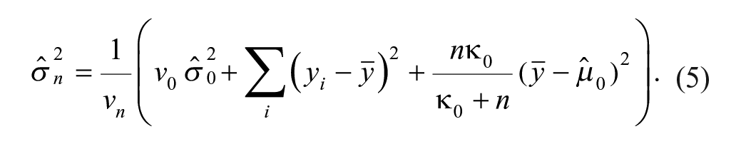
A Bayesian β-expectation tolerance interval is the interval that is expected to cover the β proportion of future observations. The one developed in this article is based on the observed variability of the analytical method and obtained by extracting quantiles from the predictive distribution (distribution of plausible future observations given the observed data). Typically, such distributions are described with a location (e.g., mean in normal distribution), a scale (e.g., variance in normal distribution), and a degrees-of-freedom parameter, which are estimated from the data. Because information collected on the study compound is limited, an obvious possibility is to move away from the classical approach and go to the Bayesian framework, where prior knowledge collected through reference compounds can be combined with the observations of the study compound to derive this predictive distribution (see the Supplemental Material). The reference compounds should not be used to provide clues about the location, as each compound has its own activity, but it can teach something about the assay variability if we have multiple observations. In the actual context, the predictive distribution (Eq. [4]) follows a t-distribution, with the mean imputed from the observations of the study compound and variance (Eq. [5]) estimated from both the reference compound (Eqs. [2]–[3]) and the study compound data (full derivation; see the Supplemental Material).
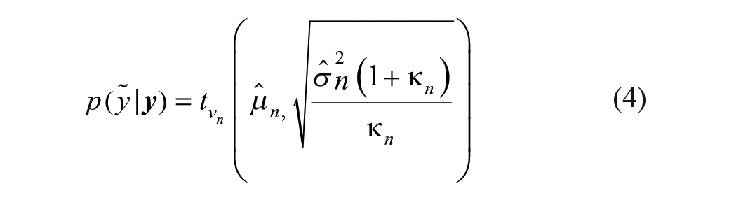
where
With no prior information on the study compound mean, ˆm0 and
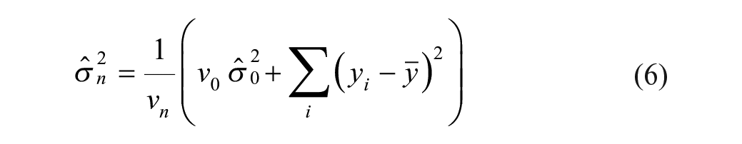
Note that this is applicable only when there is no prior information on the mean of the study compound.
Shiny app
A shiny application (R code in supplemental material) was developed to facilitate and illustrate the computation of the compound-specific β expectation tolerance interval for end users. It is available via https://apps.arlenda.com/CompoundAlertApp/ and requires the following as input:
Intermediate precision (referred to as the prior sd) of the assay estimated from a set of reference compounds using Eq. (2) and Eq. (3) (see the Intermediate Precision Model section); a minimum of three reference compounds with six repeats each
Number of historical reference compounds and observations used in estimating prior sd (required minimum is 3 × 6 = 18)
The study compound log potency estimate(s)
When all fields are filled, the limits are computed, and different distributions that build up the predictive distribution are graphically displayed (see the Results section).
Description data
For illustration purposes, two different assays, X and Y, were used with different variabilities. A set of three reference compounds from each assay was selected to span the range of the assay. Six repeats each measured across different experiments were selected at random. These were real cell-based assay data observed in practice, which are anonymized for confidentiality reasons.
Results
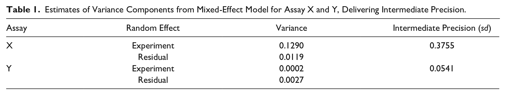
When using Bayesian β−expectation tolerance intervals, the first point of investigation in the evaluation of the reproducibility of potency estimation is defining the prior knowledge on the variability of the compound-testing procedure (see the Materials and Methods section). This variability, referred to as intermediate precision, cannot be estimated from limited data points on the study compound of interest but is estimated using the log10 potency estimates (log10 AC50) of reference compounds. To obtain a reliable intermediate precision estimate, a minimum of six experiments has been recommended. 5 This recommendation is hereafter evaluated based on historical data from seven different assays ( Fig. 1 ). It could be deduced that the recommended six repeats/experiments 5 should be enough to have a reliable estimate of the assay’s intermediate precision. The result shows that intermediate precision estimates fluctuate less after six repeats/experiments, whereas increasing the number of compounds does not improve the profiles to a large extent. It is further advised to use at least three different compounds, ideally with different potency estimates, to capture the full activity range and possible heterogeneity across the activity space so to obtain an overall average. Figure 2 presents two examples based on a real cell-based assay data, assay X and Y (see the Materials and Methods section), in which three reference compounds are selected and, for each, six repeats were randomly selected. The intermediate precision (sd) calculated based on six repeats of these reference compounds delivers prior information on expected assay variability ( Table 1 ). Based on the spread of the log10 AC50 per compound ( Fig. 2 ), one could conclude that assay Y is better under control than assay X, which is directly captured by the intermediate precision estimates (see Table 1 ). In addition, between-compound homogeneity can also be visually observed, indicating that the variability does not depend on the AC50 estimate in these particular examples.
Estimates of Variance Components from Mixed-Effect Model for Assay X and Y, Delivering Intermediate Precision.
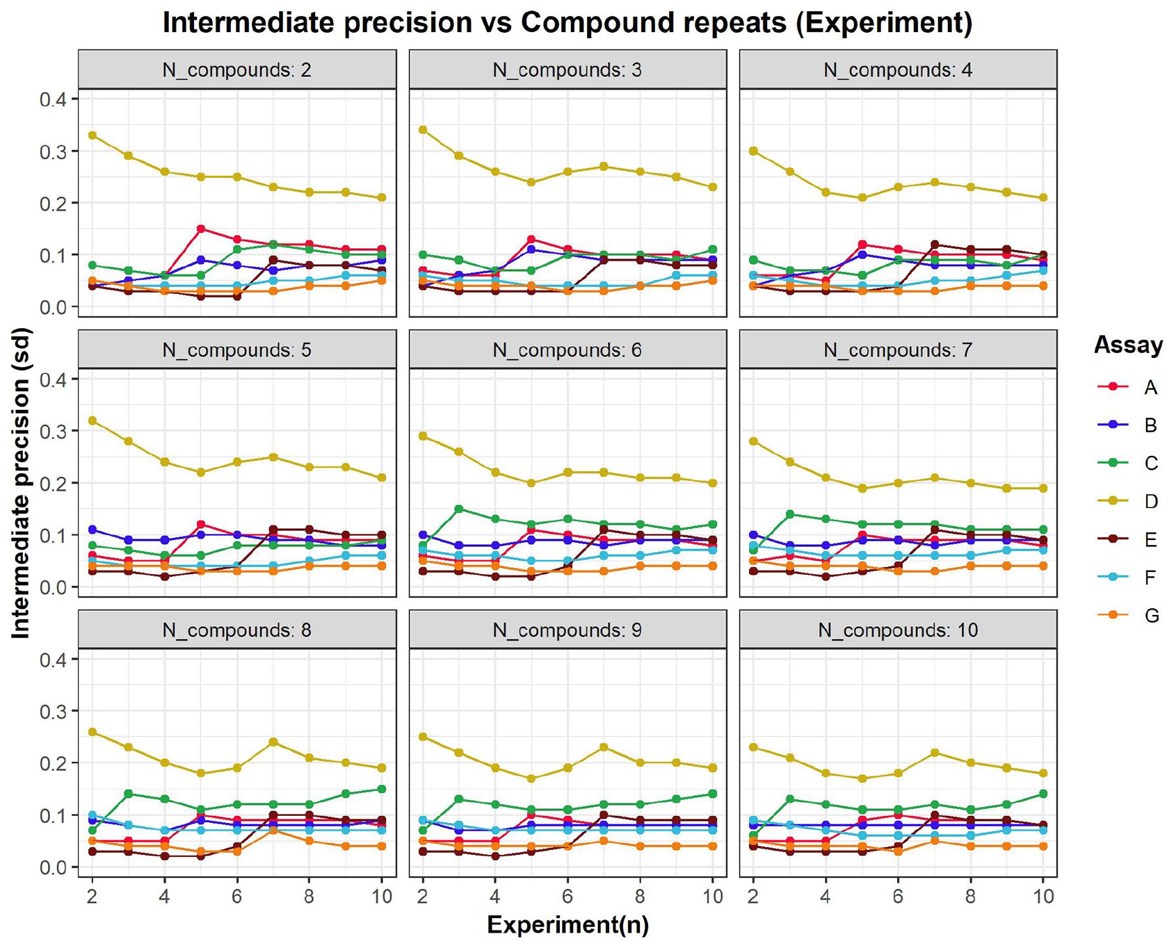
Plot of the assay intermediate precision in function of the number of experiments. The number of compounds involved in the calculation range from 2 to 10 (different panels), and different assays are indicated by different colors. The visual assessment confirms that the intermediate precision estimate stabilizes in general after six repeats when a minimum of three reference compounds are used. Please see article online for color figure.
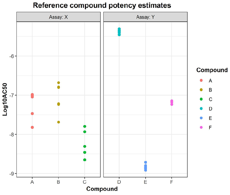
Scatter plot of log potency estimates of reference compounds from assays X and Y. The intermediate precision (sd) used as a priori for assay variance was estimated using compounds A, B, and C for assay A and compounds D, E, and F for assay Y. Please see article online for color figure.
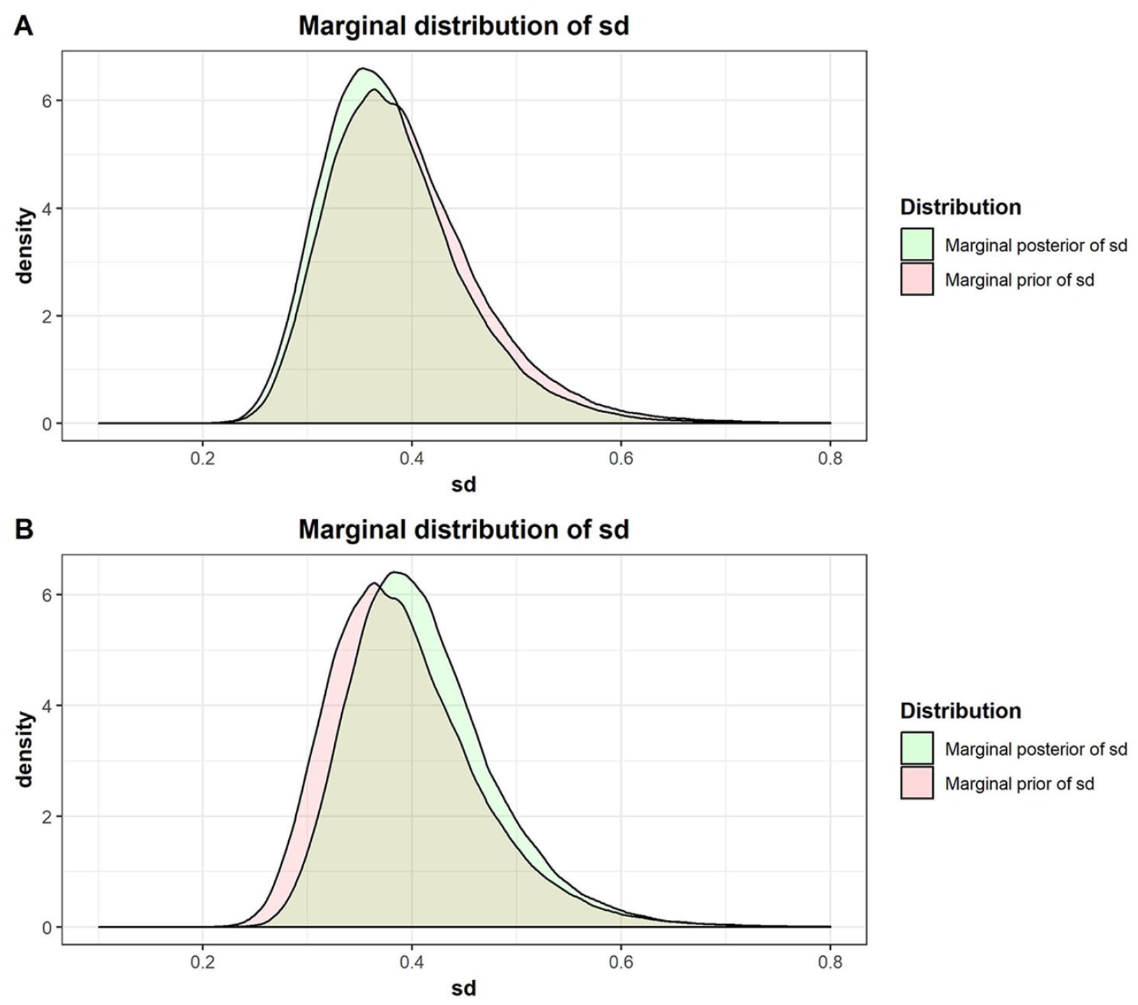
Within the Bayesian framework, the intermediate precision, capturing the expected assay variability and used as prior data, can be combined with the study compound data to derive compound-specific limits expressing the expected deviation of the estimates. Two different scenarios are considered for illustration purposes. At first, only one test result of a study compound exist in the database (i.e., Compound C is the study compound tested in assay X with a log10 AC50 equal to −5.2). Following the presented Bayesian methodology, a β-expectation tolerance interval is computed by combining the expected variability from reference compounds (prior) with the study compound test result. Figure 3A shows the distributions of the estimated sd. The red distribution is the prior belief of the assay variability solely estimated from the reference compound. This distribution is updated using the study compound data, called posterior distribution (green distribution). This sd posterior distribution is almost identical to the prior because there is only one observation present, and hence, only a small amount of information can be retrieved on the expected variability of potency estimates across experiment.
(
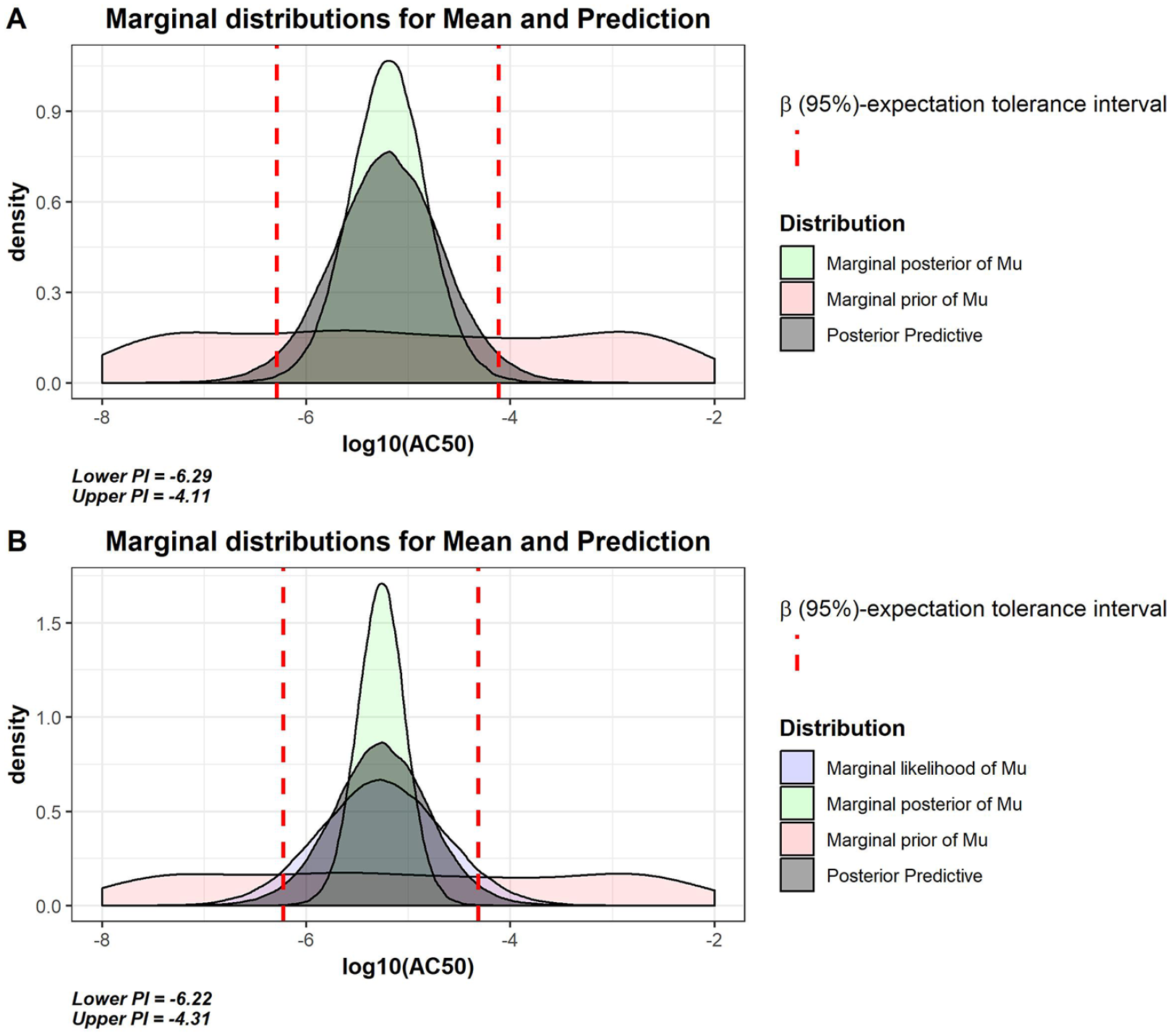
The compound-specific limits are obtained from the predictive distribution of compound C log potency described by the posterior distribution (prior + data) on the variability (sd; green distribution in Fig. 3A ) and a location parameter, delivered by the existing study compound potency estimate in database. This compound C predictive distribution follows a scaled t-distribution with 18 (n-1 with n = (3 × 6) + 1) degrees of freedom denoted as follows (see the Supplemental Material for the derivation):

Figure 4A shows the predictive distribution (dark gray) of compound C future observations based on a single previous potency estimate. The β (95%)–expectation tolerance interval was then computed as the 0.025 and 0.975 quantile of the predictive distribution and resulted in the following limits: [–6.29; –4.11]. A new observation for compound C within these limits is therefore considered to be within the normal variability range of the assay.
(
Second, let us consider an example in which more historical information is available for study compound C, namely, three historical test results (their log10 AC50 being {–5.2, –5.9, –4.7}). While the prior sd belief (red distribution in

Figure 4B shows the predictive distribution of compound C (dark gray) future observations based on three previous potency estimates, from which the compound-specific limits are derived [–6.22; –4.31], being the 0.025 and 0.975 quantiles. The accepted range of potency estimates is slightly larger compared to the first example, as the observed variability among the three estimates of compound C is slightly bigger than the prior belief based on the reference compounds. Hence, the predictive distribution has been updated using the study compound observed data.
In the next paragraph, it is assumed that three test results of compound C {–5.2, –5.9, –4.7} were observed in assay Y. Given the variability among these results, observation of such variability is more likely in assay X than in assay Y ( Fig. 2 ). Nevertheless, the β (95%)–expectation tolerance interval of compound C when observed in assay Y was computed for illustration purposes. The limits were [–5.36, –5.04] based on a single existing potency estimate and [–5.74, –4.79] based on three existing potency estimates of the study compound (see the derivation and plots in the Supplemental Material). In general, the limits are narrower compared with those derived from assay X. This is because the prior belief, estimated on the reference compounds, is much narrower. Obviously, the effect is much more pronounced when only one estimate of compound C is considered, as here the variability of the predictive distribution is driven only from the reference compounds (i.e., only the assay intermediate precision).
The above examples show that the information borrowed from the reference compounds is constantly updated as more information is acquired with subsequent repeats of the study compound. Although all expected variability is derived from the reference compound in the case of only one datapoint in the database, this variability will be updated when more information on the study compound becomes available. With more repeats, the posterior variance would converge to the true variance, and the proposed solution will be equivalent to a prediction interval calculated using the mean and variance of the observed data only. Indeed, when historical data are sparse and the actual test results are substantial, it is logical that the latter weights much more in the posterior distribution.
False Alerts
With every testing method, there is always a risk of having a false-positive result, and this is known as a type I error in statistics. A false-positive result in this case would be to have an alert for incomparability, whereas the compound potency estimates are comparable. A reasonable question to ask is how often test results are expected to fall outside the limits given that the assay is under control. In other words, what is the probability of observing a false alert? The proposed methodology involves the computation of β-expectation tolerance intervals with a 95% confidence per compound, meaning the type I error or error rate is controlled at 5% (100%–95%). In addition, the study compounds are assumed to be independent from each other, and as such, the chance of observing a false alert given that the assay is under control is 5% for each tested compound. Therefore, when this methodology is applied in an experiment in which more than one check is performed, the number of false alerts is expected to follow a binomial distribution, with probability p equal to the error rate (P = 0.05). For example, if 100 compound-specific limits are calculated during a screening campaign, there is about a 38% chance of observing more than five false alerts and a 6% chance of observing more than eight false alerts. The expected number of false alerts also depends on the predefined error rate. For instance, 98% β-expectation tolerance intervals control the error rates at 2%. In this case, the chance of observing more than five false alerts (for one compound) is reduced to about 1.6%.
Discussion
Bayesian β-expectation tolerance intervals are not new, but to our knowledge, this is the first time they have been used to evaluate future potency estimates of a compound. These β-expectation tolerance intervals, also known as prediction intervals in the frequentist setting, are ideal to evaluate future observations, but they require a reasonable amount of data before valuable compound-specific limits can be obtained. Furthermore, the Bayesian framework allows calculating these acceptance limits from the first repeat of the compound onward by borrowing information on the expected variability of the assay through some reference/quality control compounds. These limits would eventually converge to classical prediction intervals as more data on the compound itself are collected. Capturing the expected variability is preferred over some fixed thresholds, such as 0.5 log10 change, to account for differences in the performance of assays, with some having more intrinsic variability than others. In addition, in the current proposal, there is no need to summarize the historical information (e.g., mean potency estimate) before comparison, which is needed as well with the fixed threshold approaches.
How many estimates can be outside the limit while the assay is still under control is a reasonable question to ask and is controlled by defining the error rate in the β-expectation tolerance interval, where 95% intervals allow 5% chance of observing a false alert provided the assay is under control for each compound. Importantly, during screening campaigns, these limits will be calculated for all study compounds that are repeated, and these multiple tests would inflate the expected number of false alerts because of multiplicity issues. This number can be lowered if the intervals are controlled at lower error rates (e.g., 98% β-expectation tolerance intervals). However, this is at the cost of having wider limits and hence a greater chance of missing a true alert (loss of sensitivity). Fixing the appropriate error rate might depend on the stage of the discovery progress and on the risks an experimenter is willing to take.
Currently, building β-expectation tolerance intervals on AC50 test results has been proposed. However, a similar idea can be expanded to other parameters used to define potency estimates, such as minimum effective concentration and point of departure weighted entropy score (PODWES). 17 Both are used as measures to estimate the concentration at which a compound induces a specific effect on its target. The former is defined as the minimum concentration of a compound at which a desired response is observed, and the latter is the concentration that produces the maximum rate of change in entropy along the concentration-response profile. 17 Like AC50, these metrics are used to rank compounds based on their activities, and as such, it is desired to ensure stable estimates across experiments. The strength of the proposal is to build (early) compound-specific limits considering the variability of the assays by using the variability of reference compounds as a priori knowledge on the expected variability.
Supplemental Material
Supp_Material4Controlling_reproducibility_of_AC50_estimation_through_Bayesian_beta_expectation_tI – Supplemental material for Controlling the Reproducibility of AC50 Estimation during Compound Profiling through Bayesian β-Expectation Tolerance Intervals
Supplemental material, Supp_Material4Controlling_reproducibility_of_AC50_estimation_through_Bayesian_beta_expectation_tI for Controlling the Reproducibility of AC50 Estimation during Compound Profiling through Bayesian β-Expectation Tolerance Intervals by Wilson Tendong, Pierre Lebrun and Bie Verbist in SLAS Discovery
Footnotes
Acknowledgements
The authors would like to thank the Janssen R&D team for providing us with cell-based assay data for the analysis.
Supplemental material is available online with this article.
Declaration of Conflicting Interests
The authors declared no potential conflicts of interest with respect to the research, authorship, and/or publication of this article.
Funding
The authors disclosed receipt of the following financial support for the research, authorship, and/or publication of this article: Wilson Tendong and Pierre Lebrun were employees of Pharmalex Belgium and Janssen R&D (Bie Verbist). Additional financial support was provided by Janssen R&D for the research, authorship, and publication of the article.
References
Supplementary Material
Please find the following supplemental material available below.
For Open Access articles published under a Creative Commons License, all supplemental material carries the same license as the article it is associated with.
For non-Open Access articles published, all supplemental material carries a non-exclusive license, and permission requests for re-use of supplemental material or any part of supplemental material shall be sent directly to the copyright owner as specified in the copyright notice associated with the article.