Sage Journals: Discover world-class research

Abstract

Urban homelessness is a complex issue rooted in structural inequalities and spatial disparities, significantly affecting urban life and well-being. Existing research often relies on survey-based or linear regression methods, which are limited in scope, coverage, and their ability to capture nonlinear associations. This study addresses these gaps by combining homeless incident reports from New York City’s 311 service with multi-source urban big data and employing a Light Gradient Boosting Machine (LightGBM) model alongside SHapley Additive Explanations (SHAP). Through a census tract-level analysis, we examine how socioeconomic, built environment, transportation, and urban landscape factors relate to homelessness incidence. Our findings show that (1) the importance of predictive factors varies across location types, for instance, information, and communication POIs are most predictive in commercial areas, while felony crime and median income dominate in residential zones; (2) socioeconomic and built environment features are consistently more important than transportation and visual landscape indicators; and (3) many factors exhibit nonlinear relationships and threshold effects, such as sharp increases in homelessness beyond a median rent of $1800 or Gini index of 0.53. These findings offer new insights into the spatial distribution and drivers of homelessness and underscore the value of interpretable machine learning in urban analytics. By identifying key environmental thresholds, this study provides evidence-based guidance for spatially targeted urban interventions, such as prioritizing support services in high-risk areas and designing inclusive public spaces that can help mitigate homelessness and promote more sustainable and equitable cities.

Keywords

Homelessness urban big data street view imagery interpretable machine learning SHapley additive explanations

Introduction

Urban homelessness is a pervasive and complex issue that underscores profound socioeconomic disparities and significantly impacts the quality of urban life globally (Ford et al., 2014; Fowle, 2022). It not only presents a socioeconomic challenge but also poses a severe humanitarian crisis, influencing public health, safety, and urban social dynamics (Majumder et al., 2023; Onapa et al., 2022). This issue is particularly severe in the global metropolis like New York City (NYC), NYC sheltered approximately 85,677 individuals nightly as of July 2023, showing the stark contrast between the affluent cityscape and the plight of those without stable living conditions (Homeless, 2019).

Apart from its visible manifestations, homelessness also has severe consequences on the economy (Anguche, 2024; Quigley and Raphael, 2001), society (Constantinescu and Brasoveanu, 2020; Schütz, 2016), and public policy (Hill, 1994; Kiesler, 1991). It is reflective of the breakdown of housing markets, social welfare systems, and city management, often calling attention to the disparities in the allocation of wealth, health, and opportunity (Cleveland, 2020; Dobson, 2022; Hennigan, 2017). Homelessness is also associated with increased rates of chronic illness (Bensken et al., 2021; Lewer et al., 2019), mental illness (Currie et al., 2014; Folsom et al., 2005), and exposure to environmental hazards (Goodling, 2020; Van et al., 2024), placing disproportionate pressure on public health programs and emergency services. Economically, it represents both direct economic costs, through increased utilization of shelters, hospitals, and law enforcement (Berk and MacDonald, 2010; Hwang et al., 2011; Klaassen et al., 2022; Salit et al., 1998), as well as indirect costs, including decreased labor force participation and productivity (Tam et al., 2003; Zlotnick et al., 2002). In addition, chronic homelessness also erodes public trust in urban institutions and challenges the legitimacy of policies claiming to ensure inclusive and equitable development (Willison, 2021). Understanding the drivers of homelessness is thus not only a matter of empirical analysis, but also a pressing policy priority in the pursuit of sustainable, just, and resilient cities.

Homelessness is influenced by a variety of urban factors that often interact in complex ways (Mago et al., 2013; Shelton et al., 2009). For instance, socioeconomic disparities such as income inequality and unemployment may exacerbate housing affordability issues, forcing individuals into unstable living conditions (Foster and Kleit, 2015; Stansfield and Semenza, 2023; Zhu et al., 2023). At the same time, the built environment, including land use patterns and transportation infrastructure, interacts with socioeconomic variables to shape access to essential services and opportunities (Derrien et al., 2023; Jocoy and Del Casino Jr., 2010). For example, areas with high median rents and limited public transportation options may disproportionately impact low-income individuals, creating environments where homelessness is more likely (Barton and Gibbons, 2017; Bocarejo et al., 2014). Similarly, urban landscapes, such as green spaces, can mitigate stress or exclusion but may also overlap with socioeconomic factors like crime density, influencing whether these spaces are accessible to vulnerable populations (Bogar and Beyer, 2016; Rose, 2019). The complexities of homelessness require thorough investigation, particularly within urban contexts where diverse factors interplay. Therefore, NYC’s substantial homeless population and the intricate urban dynamics provide a valuable context for exploring the nonlinear relationships and threshold effects between various urban environmental factors and homelessness.

Previous studies investigating the factors affecting homelessness have often relied on surveys and questionnaires, which are limited by respondent bias and incomplete data coverage (Nishio et al., 2017; Racionero-Plaza et al., 2021). Additionally, these studies tend to focus on individual aspects of homelessness rather than exploring how different environmental factors interact to shape homelessness dynamics. For example, Wusinich et al. (2019) used interviews with 43 unsheltered homeless individuals to examine their challenges in accessing public services, revealing a preference for staying in subway stations to stay warm during cold weather. The 1996 National Survey of Homeless Assistance Providers and Clients (Aron, 2002) found that 30% of unsheltered homeless participants sell recyclables or belongings to make money, highlighting the appeal of commercial areas. Furthermore, existing research often uses traditional linear regression models, such as Ordinary Least Squares (OLS), which can only reveal linear relationships. Ee and Zhang (2022) employed OLS and Geographically Weighted Regression (GWR) to examine the global and local relationships between homelessness and crime, while Jarvis (2015) used OLS and interviews to show the negative effect of Check-In Centers on homelessness. There remains a significant gap in utilizing multi-source urban environmental data and nonlinear regression methods to better investigate these factors and associations.

Unlike traditional linear regression models, machine learning (ML) models can capture the nonlinear relationships between environmental factors and homelessness. Recent advancements in ML, including models like Random Forest (RF), eXtreme Gradient Boosting, and Light Gradient Boosting Machine (LightGBM), have proven effective in processing multi-source big data and uncovering complex relationships in homelessness studies (Chen et al., 2024; VanBerlo et al., 2021; Walters et al., 2021). However, these models often face a trade-off between predictive accuracy and interpretability, leading to the challenge of the “black box” effect, where understanding the local impact of each variable becomes difficult (Doshi-Velez and Kim, 2017; Rudin, 2019).

To address the “black box” issue, interpretable machine learning (IML) methods have emerged to clarify the decision-making processes of advanced models (Adadi and Berrada, 2018). Techniques such as SHapley Additive exPlanations (SHAP) (Lundberg and Lee, 2017), Local Interpretable Model-agnostic Explanations (Ribeiro et al., 2016), and Partial Dependence Plots (Friedman, 2001) aim to offer transparency and insight into ML models. SHAP, based on cooperative game theory, has become a preferred method in urban studies for its ability to provide both global and local interpretability (Deb and Smith, 2021), crucial for identifying key factors influencing complex issues like homelessness (Kim and Lee, 2023; Yi et al., 2024). While VanBerlo et al. (2021) used an ML approach to predict chronic homelessness and explored contributing factors, their study did not account for unsheltered homeless individuals or examine the nonlinear and spatially heterogeneous relationships. Additionally, few studies have compared the relative importance of environmental features across location types or identified specific impact thresholds.

To address these gaps, this study leveraged multi-source urban big data and IML to explore the relative importance of features, and the nonlinear relationships between environmental factors and different location types of homelessness. Specifically, we aimed to answer the following research questions: (1) Do the contributions of environmental features vary across different location types (e.g., street, commercial, and residential), and what patterns emerge across these contexts? (2) What is the overall relative importance of socioeconomic, built environment, transportation, and visual landscape features in explaining homelessness? (3) What nonlinear and threshold effects exist in the relationship between these features and homelessness incidence, and how can they help interpret spatial variations in vulnerability?

Related works

Socioeconomic and built environment determinants of urban homelessness

Homelessness is a multifaceted social issue, variously defined and conceptualized across disciplines. The U.S. Department of Housing and Urban Development (HUD) defines homelessness as the condition of individuals lacking a fixed, regular, and adequate nighttime residence, encompassing those living in shelters, transitional housing, cars, abandoned buildings, and public spaces. Similarly, the European Typology of Homelessness and Housing Exclusion (ETHOS) distinguishes between rooflessness, houselessness, and inadequate housing (Amore et al., 2011). The World Health Organization (WHO) also introduces the concept of “hidden homelessness,” which includes individuals without a secure place to live who are not visibly residing on the streets or in shelters. Despite these variations in definition, the common thread is a lack of stable housing. Our study aligns with these definitions, examining both encampment homelessness, where individuals establish makeshift residences in public spaces, and general homelessness, representing those without secure housing.

Existing literature has extensively examined how socioeconomic factors contribute to homelessness, primarily identifying correlational relationships, though some studies have also articulated causal mechanisms. Income inequality and poverty rates are consistently linked with higher homelessness incidence, as economic disparities reduce housing affordability, pushing vulnerable populations into unstable living situations (O’flaherty, 1996; Byrne et al., 2021; Sharam and Hulse, 2014). Lower educational attainment has been causally linked to higher homelessness risk due to diminished economic mobility and reduced access to stable employment opportunities (Parrott et al., 2022). Furthermore, neighborhood racial and demographic composition impacts homelessness incidence through systemic inequalities affecting access to housing, employment, and social support (Fowle, 2022; Fusaro et al., 2018). Crime rates exhibit a complex, primarily positive relationship with homelessness; higher crime density can foster socioeconomic instability, discourage local investment, and reduce social cohesion, indirectly exacerbating homelessness (Berk and MacDonald, 2010; Ee and Zhang, 2022; Kelling and Bratton, 1997). For example, Fischer et al. (2008) found that homelessness, particularly when accompanied by psychological distress, causally increases both non-violent and violent crime rates, highlighting a reciprocal relationship that exacerbates homelessness conditions. Similarly, substance abuse, economic hardship, and weakened social networks are documented as interconnected causal pathways that lead individuals toward homelessness (Batterham, 2019; Bradford and Lozano-Rojas, 2024; Vangeest and Johnson, 2002).

Regarding the built environment, studies suggest both direct and indirect relationships with homelessness incidence. Land use patterns and urban functions directly shape service availability, influencing housing options and service accessibility for homeless populations (Kuhn and Culhane, 1998; Ranasinghe and Valverde, 2006). Accessibility to transportation infrastructure shows a nuanced relationship; higher accessibility is typically positively correlated with homelessness, as these areas offer greater mobility, resource access, and shelter options, thereby attracting vulnerable populations (Canham et al., 2023; Jocoy and Del Casino Jr., 2010; Murphy, 2019). Conversely, proximity to police stations often has an inverse correlation, as homeless individuals may avoid areas with increased surveillance and eviction risks (DePastino, 2003; Rossi, 1991). Urban visual features, derived from street-level imagery, offer additional insights. Empirical studies suggest that urban green spaces (UGS) can improve mental well-being and reduce environmental stressors (Li et al., 2015; Wang et al., 2025). UGS are of great significance for people experiencing homelessness not merely as a necessity or last resort, but more importantly as spaces that align with individual preferences and help fulfill personal needs (Koprowska et al., 2020). Walkability, reflecting pedestrian-friendly urban design, has shown a negative correlation with homelessness as walkable areas typically foster social cohesion and support networks, indirectly mitigating homelessness vulnerability (Frank et al., 2006; Speck, 2018). Urban enclosure, indicating dense building configurations and limited open spaces, generally positively correlates with homelessness due to providing sheltered and discrete locations preferred by homeless populations (Ma et al., 2021; Sewell, 1993).

Based on the insights from prior empirical studies, our research systematically selected variables representing these theoretically and empirically established socioeconomic and built environment factors.

Applications of interpretable machine learning methods

In recent years, remarkable advancements in machine learning have given rise to sophisticated models capable of deciphering complex data relationships (Chen and Guestrin, 2016; He et al., 2016; Vaswani et al., 2017). However, this evolution often comes with a trade-off between predictive precision and model interpretability, giving rise to the notion of the “black box” (Caruana et al., 2015; Doshi-Velez and Kim, 2017; Rudin, 2019). To address this, IML methods have surfaced as an essential resolution, shedding light on the decision-making processes of these advanced models (Adadi and Berrada, 2018). These methods include a variety of techniques, such as SHapley Additive exPlanations (SHAP) (Lundberg and Lee, 2017), Local Interpretable Model-agnostic Explanations (LIME) (Ribeiro et al., 2016), and Partial Dependence Plots (PDP) (Friedman, 2001), each aiming to offer transparency and insight into the functionalities of machine learning models.

SHAP has been preferred in urban studies over methods like LIME due to its consistent and model-agnostic interpretability. SHAP is grounded in cooperative game theory (Lundberg and Lee, 2017), specifically the concept of Shapley values. It can both provide global and local interpretability (Deb and Smith, 2021) and precise explanations of model predictions, which is crucial in addressing complex issues like homelessness by identifying key contributing factors. For instance, Yi et al. (2025) combined random forest and SHAP to assess vegetated and built-up areas’ independent effects on heat exposure environment. Similarly, Kim and Lee (2023) employed urban big data, LightGBM, and SHAP to explore the nonlinear association between crime and urban environment, proposing policy implications for improving public safety and sustainability. Additionally, Hatami et al. (2023) applied SHAP to uncover the impact of the built environment on commuting mode choices, underscoring the significance of dense, diverse, and accessible regions in fostering sustainable transportation. Ji et al. (2022) employed XGBoost and SHAP to investigate nonlinear correlations and interaction effects between the built environment and cycling distance, identifying the crucial roles of road network configurations and bicycle lane facilities in shaping cycling activities. Kim and Kim (2022) formulated a random forest-based model to predict heat-related mortality in urban settings, achieving notable accuracy and pinpointing key influential factors through SHAP interpretation.

Materials and methods

The overall analysis workflow is illustrated in Figure 1. It mainly contains three parts: (1) data collection and variable preprocessing; (2) ML model construction, evaluation, and interpretation with SHAP; (3) analyzing results, including feature’s relative importance across different locations, nonlinear relationships, and threshold effects.

Figure 1.

Overall Analysis Framework. This study consists of three main parts: (1) Collect and extract features from the multi-source urban big data, including socioeconomic features, build environment, urban transportation, urban landscape, and homeless data; (2) Machine learning models’ construction, evaluation, and interpretation with SHAP; (3) Interpretation results analysis.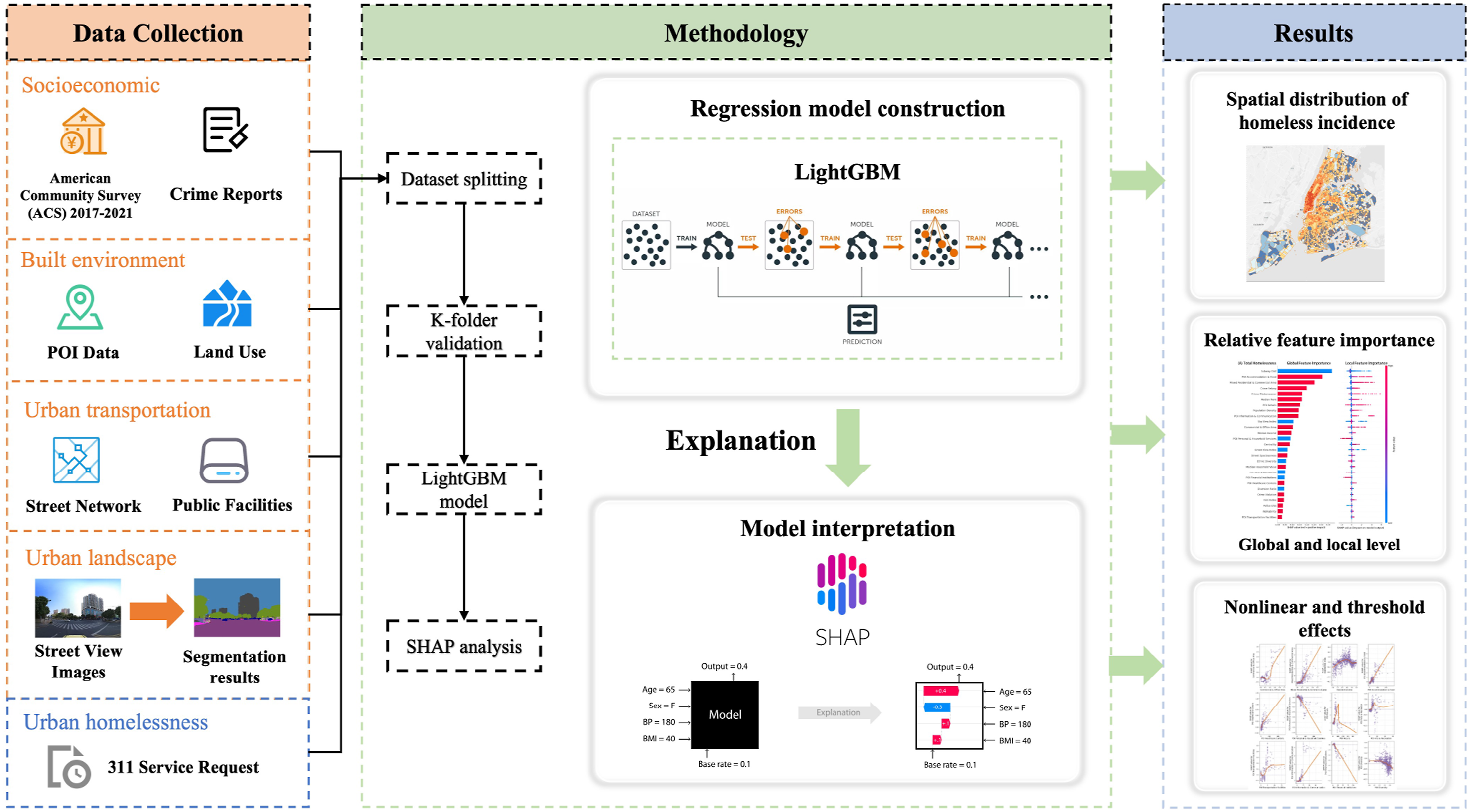

Study area and datasets

Study area

As shown in Figure 2, the study area includes NYC’s five boroughs: the Bronx, Brooklyn, Manhattan, Queens, and Staten Island. Despite its status as a populous and economically vibrant city, NYC faces a severe homelessness crisis. In July 2023, the NYC Department of Homeless Services and the Department of Housing Preservation and Development reported 85,677 individuals experiencing homelessness in the city’s municipal shelter system, including 28,540 children. Additionally, nearly 24,660 single adults sought shelter nightly during the same month. Factors such as high population density, socioeconomic disparities, housing affordability challenges, and limited access to social services exacerbate the homelessness situation in the city.

Figure 2.

Study area: five boroughs of New York City.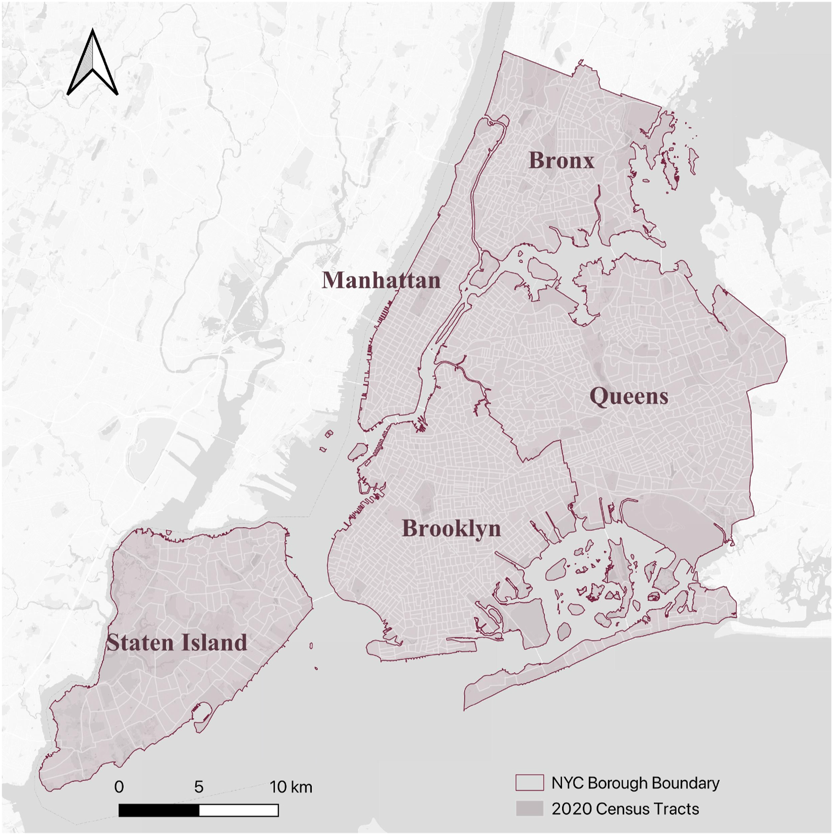

In this study, census tracts were utilized as the spatial units of analysis. A total of 1712 census tracts were included after excluding observations with null values for some variables. The average size of a census tract in is 32.65 km², and the population density is approximately 208.91 people per km². This level of granularity allowed for a detailed examination of the relationship between various environmental factors and homelessness, providing insights into the localized dynamics of homelessness within the diverse neighborhoods of NYC.

Data sources

We used data from eight key categories. The homelessness data, consisting of 42,333 records, were sourced from the NYC 311 Service Request dataset and the Department of Homeless Services for 2022. Socioeconomic indicators were drawn from the 2021 American Community Survey (ACS). The 2022 land use data from the NYC Department of City Planning included 857,006 parcels. We also used 150,575 points of interest (POI) data from SafeGraph (2021), and transit data from the General Transit Feed Specification (GTFS) covering bus and subway stations for 2022. Additionally, crime and police station data were obtained from the NYPD, and 191,894 Google Street View (GSV) images were collected during the spring and summer from 2020 to 2022. These comprehensive data sources enable a thorough analysis of homelessness in relation to neighborhood socioeconomics, the built environment, urban transportation, and urban landscape.

Model constructions

Dependent variable

The dependent variable in this study is homelessness density within each census tract, calculated by dividing the total number of reported homelessness incidences by the tract’s area. The homelessness data includes two types of reports: “calls for encampment” and “calls for assistance.” Each record contains a timestamp, location type, zipcode, address, and geographical coordinates. To ensure data accuracy and remove redundancy, we applied two deduplication rules based on time and location. Reports with identical timestamps were flagged as potential duplicates, as were those with a time difference of less than 10 minutes and matching zip codes or coordinates. We also re-categorized the location types into five groups: Street, Commercial, Residential, Park, and Others. This categorization allows us to analyze homelessness dynamics across different urban environments. Table 1 summarizes key statistics from the dataset.

Table 1.

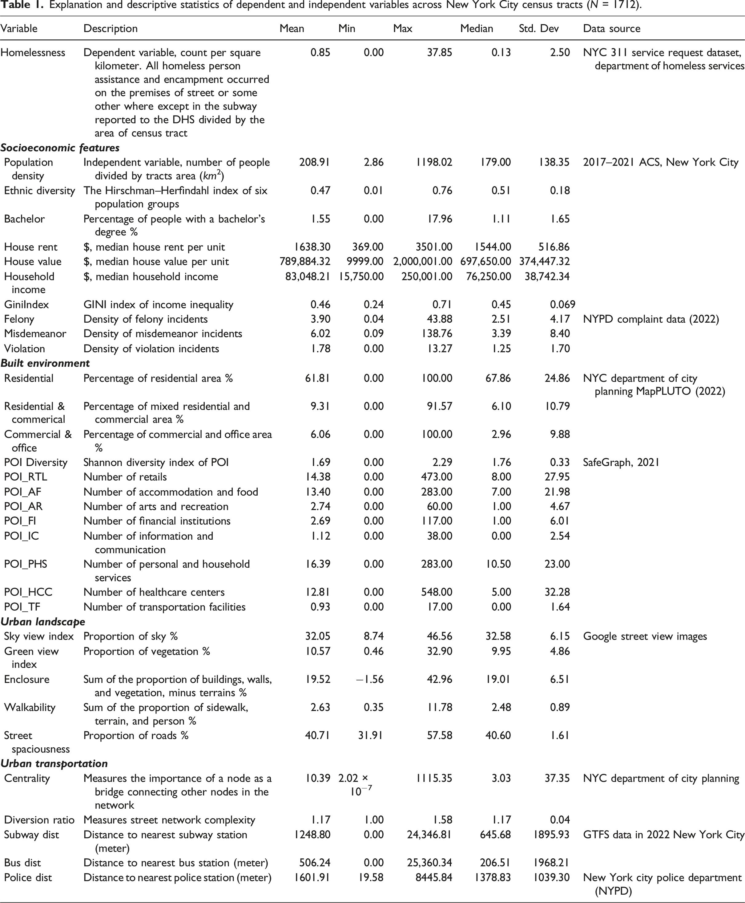
Explanation and descriptive statistics of dependent and independent variables across New York City census tracts (N = 1712).

Variable	Description	Mean	Min	Max	Median	Std. Dev	Data source
Homelessness	Dependent variable, count per square kilometer. All homeless person assistance and encampment occurred on the premises of street or some other where except in the subway reported to the DHS divided by the area of census tract	0.85	0.00	37.85	0.13	2.50	NYC 311 service request dataset, department of homeless services
Socioeconomic features
Population density	Independent variable, number of people divided by tracts area (km²)	208.91	2.86	1198.02	179.00	138.35	2017–2021 ACS, New York City
Ethnic diversity	The Hirschman–Herfindahl index of six population groups	0.47	0.01	0.76	0.51	0.18
Bachelor	Percentage of people with a bachelor’s degree %	1.55	0.00	17.96	1.11	1.65
House rent	$, median house rent per unit	1638.30	369.00	3501.00	1544.00	516.86
House value	$, median house value per unit	789,884.32	9999.00	2,000,001.00	697,650.00	374,447.32
Household income	$, median household income	83,048.21	15,750.00	250,001.00	76,250.00	38,742.34
GiniIndex	GINI index of income inequality	0.46	0.24	0.71	0.45	0.069
Felony	Density of felony incidents	3.90	0.04	43.88	2.51	4.17	NYPD complaint data (2022)
Misdemeanor	Density of misdemeanor incidents	6.02	0.09	138.76	3.39	8.40
Violation	Density of violation incidents	1.78	0.00	13.27	1.25	1.70
Built environment
Residential	Percentage of residential area %	61.81	0.00	100.00	67.86	24.86	NYC department of city planning MapPLUTO (2022)
Residential & commerical	Percentage of mixed residential and commercial area %	9.31	0.00	91.57	6.10	10.79
Commercial & office	Percentage of commercial and office area %	6.06	0.00	100.00	2.96	9.88
POI Diversity	Shannon diversity index of POI	1.69	0.00	2.29	1.76	0.33	SafeGraph, 2021
POI_RTL	Number of retails	14.38	0.00	473.00	8.00	27.95
POI_AF	Number of accommodation and food	13.40	0.00	283.00	7.00	21.98
POI_AR	Number of arts and recreation	2.74	0.00	60.00	1.00	4.67
POI_FI	Number of financial institutions	2.69	0.00	117.00	1.00	6.01
POI_IC	Number of information and communication	1.12	0.00	38.00	0.00	2.54
POI_PHS	Number of personal and household services	16.39	0.00	283.00	10.50	23.00
POI_HCC	Number of healthcare centers	12.81	0.00	548.00	5.00	32.28
POI_TF	Number of transportation facilities	0.93	0.00	17.00	0.00	1.64
Urban landscape
Sky view index	Proportion of sky %	32.05	8.74	46.56	32.58	6.15	Google street view images
Green view index	Proportion of vegetation %	10.57	0.46	32.90	9.95	4.86
Enclosure	Sum of the proportion of buildings, walls, and vegetation, minus terrains %	19.52	−1.56	42.96	19.01	6.51
Walkability	Sum of the proportion of sidewalk, terrain, and person %	2.63	0.35	11.78	2.48	0.89
Street spaciousness	Proportion of roads %	40.71	31.91	57.58	40.60	1.61
Urban transportation
Centrality	Measures the importance of a node as a bridge connecting other nodes in the network	10.39	2.02 × 10⁻⁷	1115.35	3.03	37.35	NYC department of city planning
Diversion ratio	Measures street network complexity	1.17	1.00	1.58	1.17	0.04
Subway dist	Distance to nearest subway station (meter)	1248.80	0.00	24,346.81	645.68	1895.93	GTFS data in 2022 New York City
Bus dist	Distance to nearest bus station (meter)	506.24	0.00	25,360.34	206.51	1968.21
Police dist	Distance to nearest police station (meter)	1601.91	19.58	8445.84	1378.83	1039.30	New York city police department (NYPD)

Independent variables

The independent variables in this study were selected based on a thorough review of the literature. Prior research highlights various factors influencing homelessness, including socioeconomic disparities (e.g., income inequality, unemployment, and educational attainment), built environment characteristics (e.g., land use patterns and public spaces), transportation accessibility, and urban landscape features (e.g., green spaces and public amenities) (Byrne et al., 2021; Chan et al., 2014; Jocoy and Del Casino Jr., 2010; Lin et al., 2022). To ensure comprehensive coverage of these factors, we collected a wide range of indicators, including four main categories: neighborhood socioeconomic, built environment, urban transportation and urban landscape variables. This approach allowed us to construct a holistic dataset to explore the complex and interactive relationships between urban factors and homelessness.

This study investigated neighborhood socioeconomics across five dimensions: Demographics, Education, Housing, Economics, and Crime. For Demographics, we used population density and an ethnic diversity index based on the Hirschman–Herfindahl index (De Nadai et al., 2020), which measures diversity across racial groups. The index, denoted as H, is calculated using the equation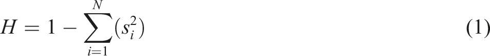

H = 1 - \sum_{i = 1}^{N} (s_{i}^{2})

(1)

where s_i is the proportion of individuals in racial group i, and N is the total number of groups. For Education, we used the proportion of individuals with a bachelor’s degree in each tract. In Housing, we considered median rent and house value to assess affordability and market conditions. The Economics dimension included the Gini index of income inequality and median income. For Crime, we used NYPD data from 2022, categorizing crimes as Violations (83,085), Misdemeanors (264,658), and Felonies (172,918), and calculated crime density across all tracts.

For the built environment, we focused on urban function and land use using SafeGraph’s POI dataset, which includes businesses and amenities categorized by the North American Industry Classification System (NAICS). This dataset provides information such as names, locations, and category codes of various establishments. We selected eight categories for analysis: retail, accommodation and food services, arts and recreation, financial institutions, information and communication, personal and household services, healthcare centers, and transportation facilities. Each POI was mapped to its census tract, allowing us to calculate the number of amenities per tract. To assess POI diversity, we used Shannon entropy, which reflects the order in both categories and the number of POIs (Yue et al., 2017). It is calculated as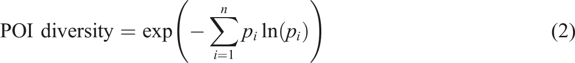

P O I d i v e r s i t y = \exp (- \sum_{i = 1}^{n} p_{i} \ln (p_{i}))

(2)

In this equation, n represents the number of POI categories. The term p_i denotes the proportion of the ith category of POI within a given census tract.

Land use plays a central role in shaping the urban environment and influences many facets of urban life. In this study, we focused on a selection of key land use categories, namely commercial & office, mixed residential & commercial, and residential, as shown in Figure 3. By examining the proportional area occupied by these various categories of land use, we aim to understand the spatial distribution and composition of diverse land utilizations.

Figure 3.

2D and 3D spatial distribution of land use in New York City.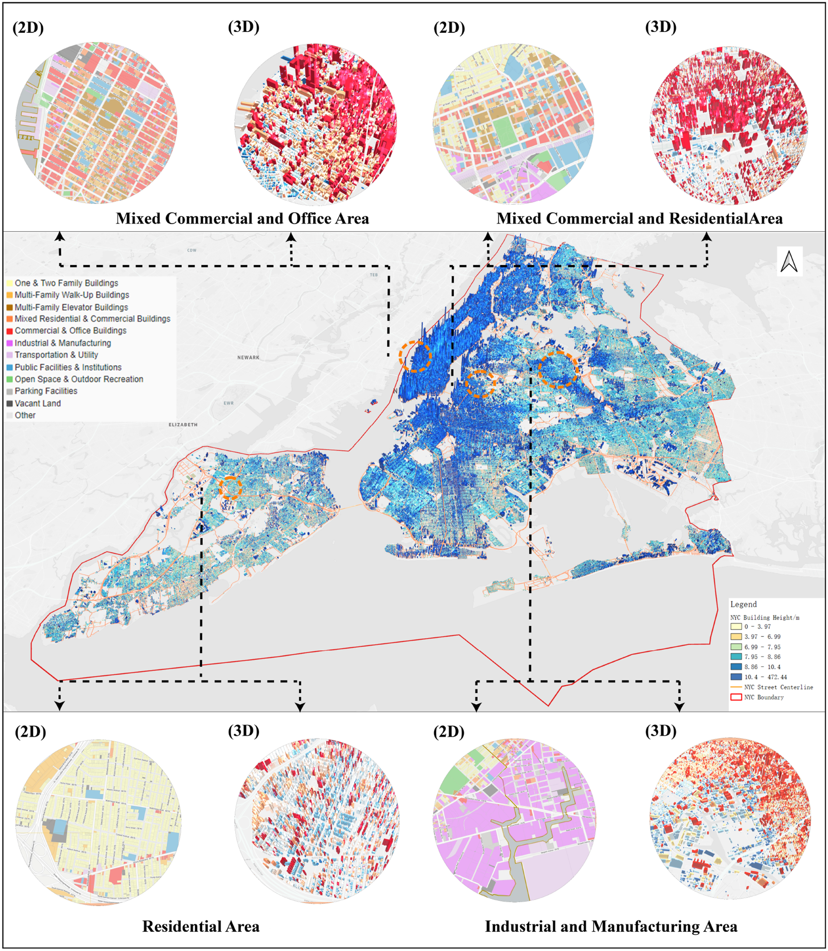

The characteristics of the street network were analyzed using sDNA (Spatial Design Network Analysis). We employed the centrality index to measure how central each street segment is in connecting other segments, quantifying its role in promoting mobility and accessibility. We also used the diversion ratio to assess the complexity and fragmentation of the street network, providing insight into the connectivity of different regions (Meng and Zacharias, 2021). To analyze accessibility to subway and bus stations as well as police stations, we calculated the shortest street network distances using Python. Centroids of each census tract were used as starting points, and the NetworkX library was employed to represent NYC’s street network, incorporating road segments, traffic directions, and road types. This method allowed us to capture spatial variations in public transit and police accessibility across NYC.

For urban landscape analysis, visual features were extracted from Google Street View images. We initially generated sampling points at 50-m intervals along the street network, and then retrieved all available image IDs within approximately 100–200 m of each sampling point using the streetview Python library (https://github.com/robolyst/streetview). All retrieved IDs were then traversed systematically to remove duplicates, ensuring comprehensive coverage. Subsequently, panoramic images were downloaded via the Google Street View API based on these unique IDs. After accounting for seasonal variations, we retained images captured during spring and summer from 2020 to 2022, yielding a final dataset of 191,894 panoramic images. Then, we used the Deeplabv3 + model (Chen et al., 2018), trained on the Cityscape dataset (Cordts et al., 2016), for semantic segmentation. This model, with an accuracy of 82.1%, classifies 19 categories, including roads, sidewalks, buildings, trees, and pedestrians, allowing us to calculate the proportions of each and derive mixed indicators. We focused on five key indicators: green view index (GVI) (Li et al., 2015), sky view index, enclosure (Ma et al., 2021), walkability (Wang et al., 2022), and street spaciousness, as described in Table 1.

Regression models

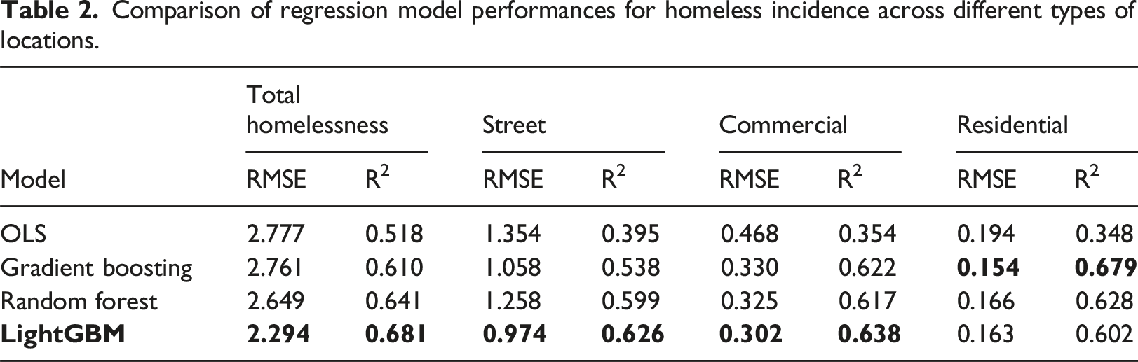
We built and compared four regression models: Ordinary Least Squares (OLS), Gradient Boosting Regression Tree (Friedman, 2001), Random Forest regression (Breiman, 2001), and LightGBM (Ke et al., 2017). The dataset was split into 80% for training and 20% for testing, and the models were validated using 10-fold cross-validation. We evaluated performance using two metrics: root mean squared error (RMSE) and the coefficient of determination (R²). RMSE measures the average deviation between predicted and actual values, calculated as

R M S E = \sqrt{\frac{1}{n} \sum_{i = 1}^{n} {(y_{i} - {\hat{y}}_{i})}^{2}}

(3)

where n is the number of data points, y_i is the actual value, and ${\hat{y}}_{i}$ is the predicted value. R² measures how well the model explains the variance in the dependent variable.

Model interpretation with SHAP

SHAP is a powerful technique for interpreting machine learning models, offering insight into the contribution of each feature to the model’s decisions. It uses the concept of Shapley values to fairly and consistently attribute feature importance, treating the model as a cooperative game with features acting as “players.” SHAP quantifies the contribution of each feature by considering all possible feature combinations and their marginal contributions, ensuring fair allocation of feature importance. This allows us to identify the key factors influencing homelessness and quantify their impact. The Shapley value of feature i, denoted as ϕ_i, is calculated as the weighted average over all possible subsets of the feature group N

ϕ_{i} = \sum_{S \subseteq N} \frac{| S |! (n - | S | - 1)!}{n!} [v (S \cup {i}) - v (S)]

(4)

Here, |S| represents the number of features in subset S, n is the total number of features in group N, v(S) is the model output for subset S, and v(S ∪ i) is the model output when feature i is added.

Results

We began by examining the distribution of homeless incidences across different locations, as shown in Figure 4. Streets and sidewalks had the highest number of reports (16,325), followed by subways (12,147). Store/commercial areas and residential houses reported 4625 and 4547 incidences, respectively. Parks/playgrounds accounted for 1977 reports, while the “Other” category had 2164. Highways, bridges, and houses of worship reported lower incidences, with 85, 72, and 391 reports, respectively.

Figure 4.

Number of homeless incidence across various locations in New York City (2022).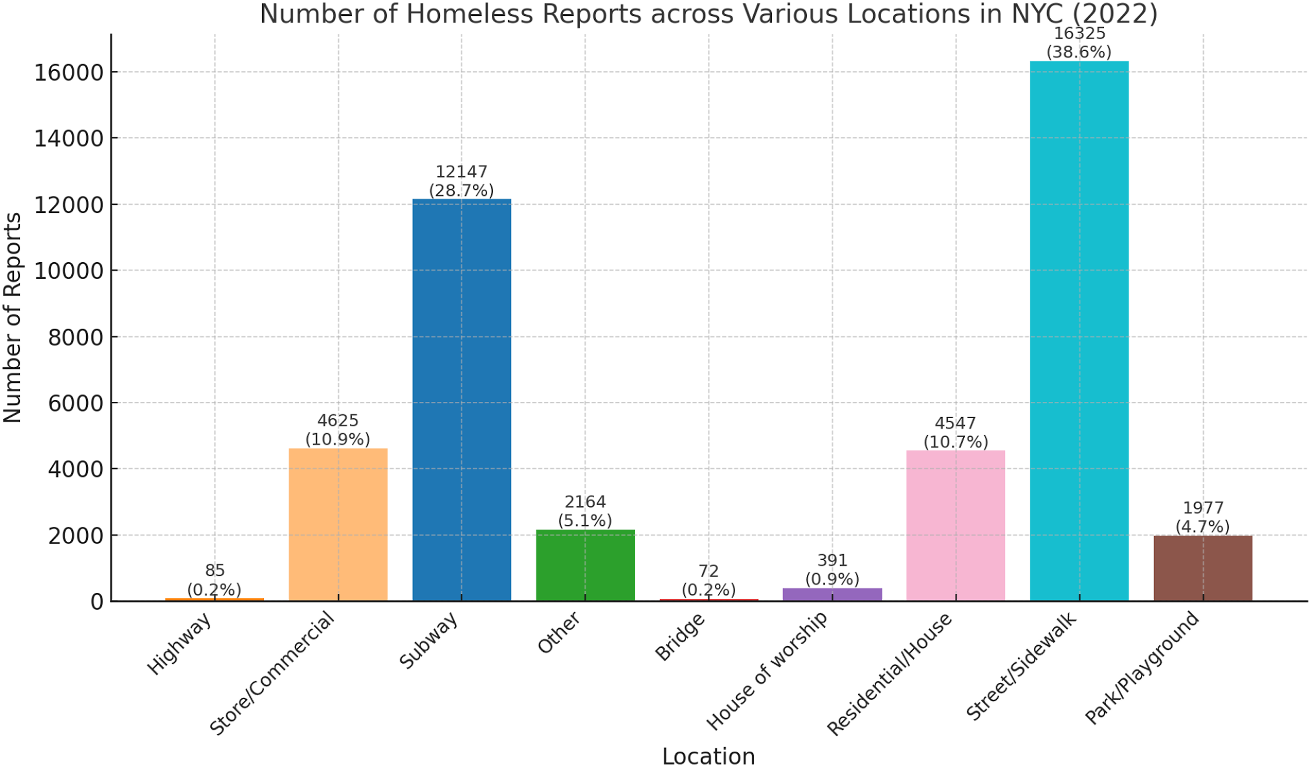

Figure 5 shows the spatial distribution of homelessness per square kilometer across census tracts. A logarithmic transformation was applied to highlight spatial patterns and reduce the effect of outliers. Darker red areas represent higher homeless density, primarily concentrated in Manhattan, with some dispersion into Brooklyn and fewer occurrences in Queens and Staten Island.

Figure 5.

Spatial distribution of homeless incidence density in New York City (2022).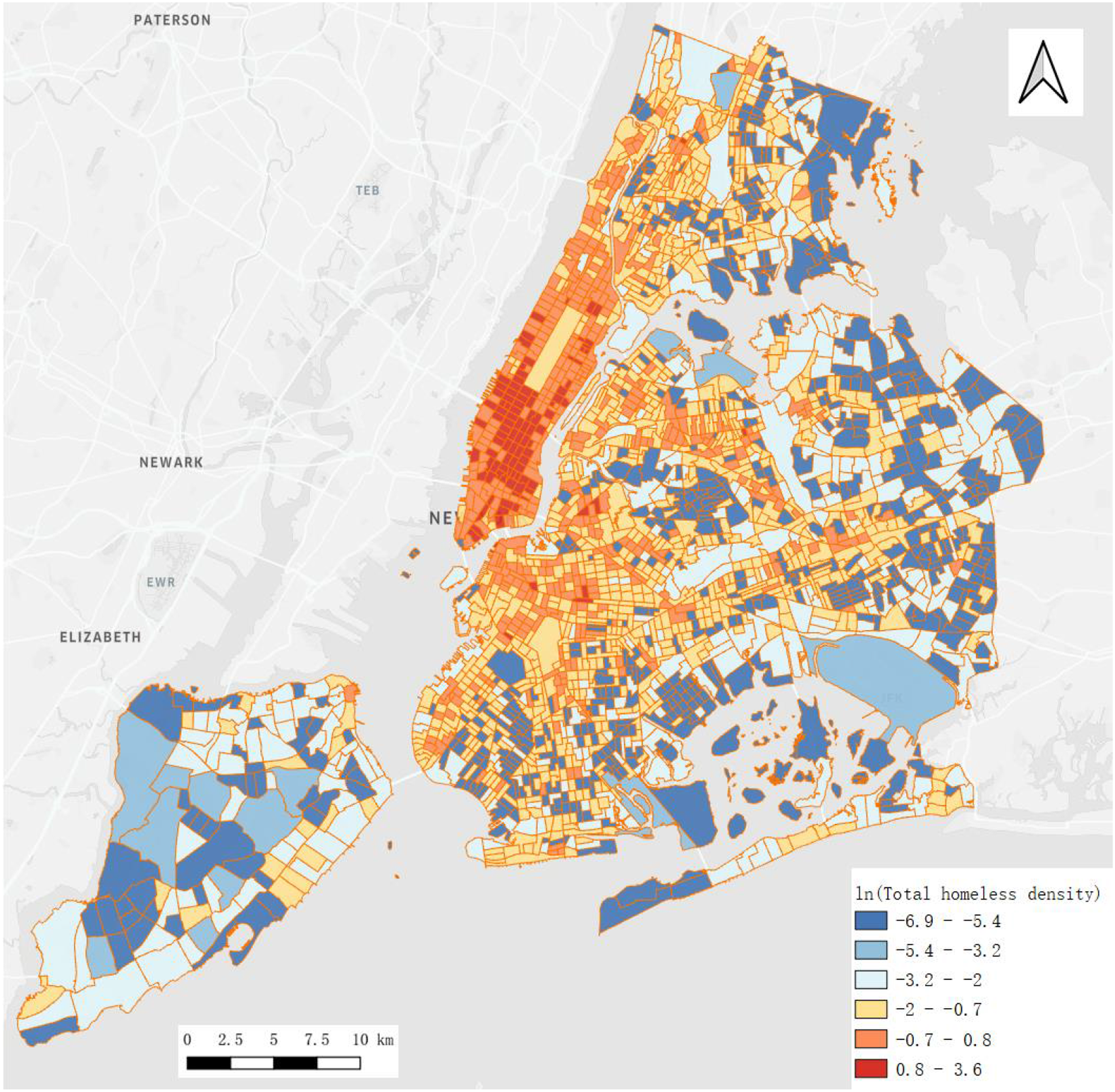

Model evaluation results

Before building the ML models, we addressed multicollinearity by eliminating variables with a variance inflation factor (VIF) greater than 5. We then used 10-fold cross-validation to evaluate model performance and parameter configurations for predicting homelessness in different location types, including total homelessness, street, commercial, and residential areas. As shown in Table 2, LightGBM consistently performed best, achieving the lowest RMSE and highest R² values across most location types. For total homelessness, LightGBM achieved an RMSE of 2.294 and an R² of 0.681, demonstrating superior predictive accuracy. LightGBM also outperformed other models in predicting homelessness for street and commercial areas, making it the optimal model for this study.

Table 2.

Comparison of regression model performances for homeless incidence across different types of locations.

Model	Total homelessness		Street		Commercial		Residential
Model	RMSE	R²	RMSE	R²	RMSE	R²	RMSE	R²
OLS	2.777	0.518	1.354	0.395	0.468	0.354	0.194	0.348
Gradient boosting	2.761	0.610	1.058	0.538	0.330	0.622	0.154	0.679
Random forest	2.649	0.641	1.258	0.599	0.325	0.617	0.166	0.628
LightGBM	2.294	0.681	0.974	0.626	0.302	0.638	0.163	0.602

Analysis of features importance in different locations

The global feature importance of variables, as shown in Figure 6, was measured using global SHAP values. Following Xiao et al. (2021), we calculated the mean absolute SHAP values (mean $|SHAP|$ ) and determined each variable’s importance by its ratio to the total mean $|SHAP|$ . Red indicates positive impacts, and blue indicates negative impacts. Figure 6 also provides local interpretations, with red dots representing higher feature values and blue dots indicating lower ones. SHAP values greater than zero have a positive influence on homelessness, while values below zero have a negative impact.

Figure 6.

Results of SHAP global and local feature importance for homelessness incidence across four location types: (a) Total Homelessness, (b) Street Homelessness, (c) Commercial Areas, and (d) Residential Areas. The left side of each panel shows global feature importance (mean absolute SHAP values), while the right side visualizes local feature importance, illustrating the positive (red) and negative (blue) impacts of each variable on homelessness incidence.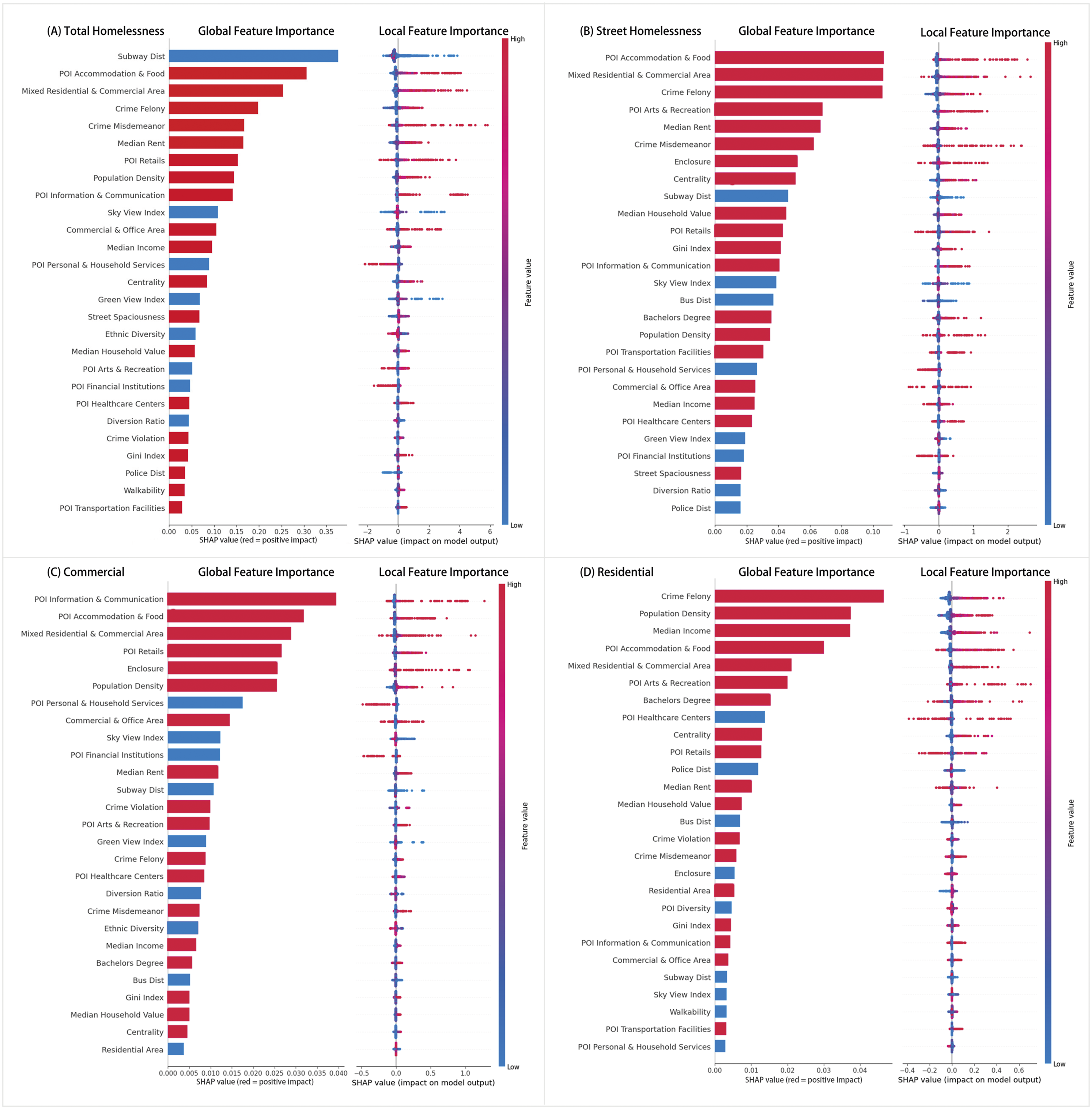

We further analyzed feature importance by location type. For total homelessness, the top five variables were subway distance, POI accommodation and food services, mixed residential/commercial areas, crime incidents, and median rent, highlighting the dominance of built environment and socioeconomic factors. Subway distance was the most important feature, which corresponds to the observed high incidence of reported homelessness in subway locations Figure 4. This likely reflects the tendency of unhoused individuals to seek shelter in areas with greater transit accessibility and foot traffic, rather than suggesting a causal effect of subway proximity on homelessness risk. For street homelessness (Figure 6(b)), the feature importance trends mirrored the overall category but with a reduced importance for subway distance. This similarity is due to street homelessness comprising the majority of cases. In contrast, commercial and residential areas showed more nuanced variations in feature importance and their impacts on homelessness.

In commercial areas (Figure 6(c)), while several top features remain consistent with the overall analysis, their impacts show notable changes. POI information and communication becomes the most influential feature. This may reflect the importance of digital connectivity for unhoused individuals seeking access to services and online resources in central urban areas. The sky view index exhibits a stronger negative association with homelessness. However, this relationship may be partly influenced by the nature of Street View imagery in commercial zones, which often feature limited sky visibility due to higher building density. Financial institutions are associated with lower reported homelessness, though this may reflect exclusionary urban environments where unhoused individuals have fewer opportunities to remain. Finally, the increased relative importance of violent crime, alongside the reduced influence of felony crime, suggests changing spatial dynamics of urban disorder in commercial zones, further investigation is needed to unpack causal mechanisms.

In residential areas (Figure 6(d)), the feature importance rankings reveal several distinct patterns. Felony crime density, population density, and median income show higher importance, suggesting these areas may host more visible or reported homelessness under specific demographic or housing conditions. Notably, homelessness appears more concentrated in medium-to-high density tracts, potentially reflecting the affordability pressures and systemic vulnerabilities in these transitional zones. The increased importance of educational attainment (bachelor’s degree) may point to broader neighborhood socioeconomic profiles, though it is unlikely to represent a direct risk factor for homelessness itself. In contrast, features such as sky view index and proximity to subway stations show decreased importance in residential zones, likely due to the more suburban character of these neighborhoods, where urban form and transit access play a lesser role in shaping homelessness visibility.

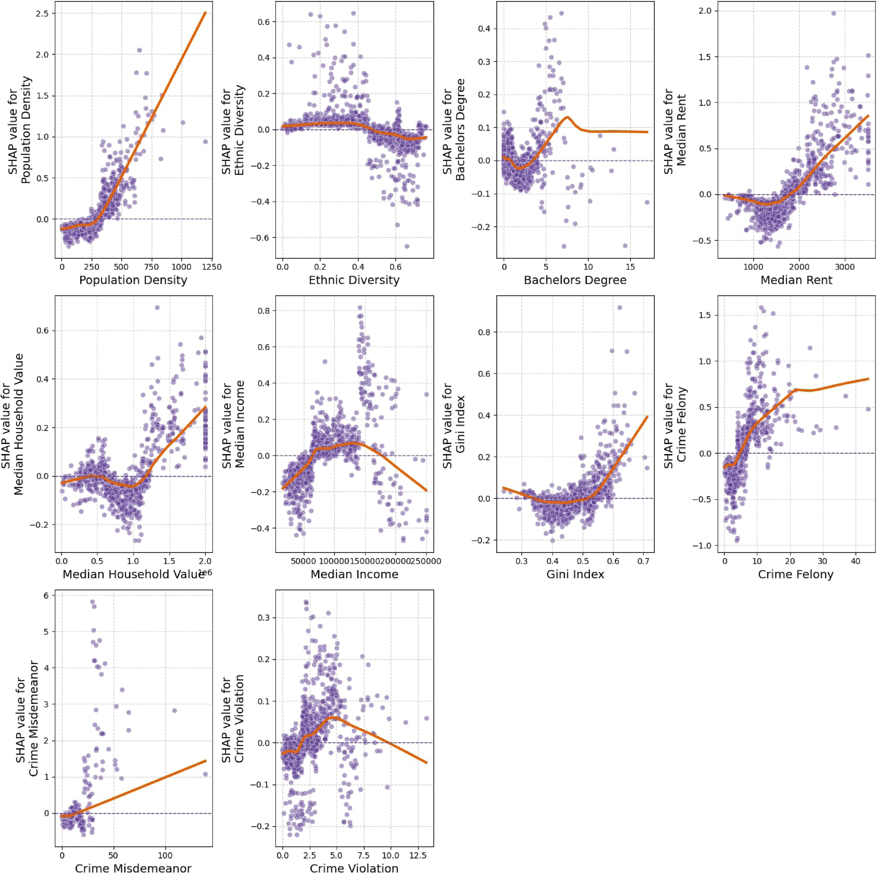
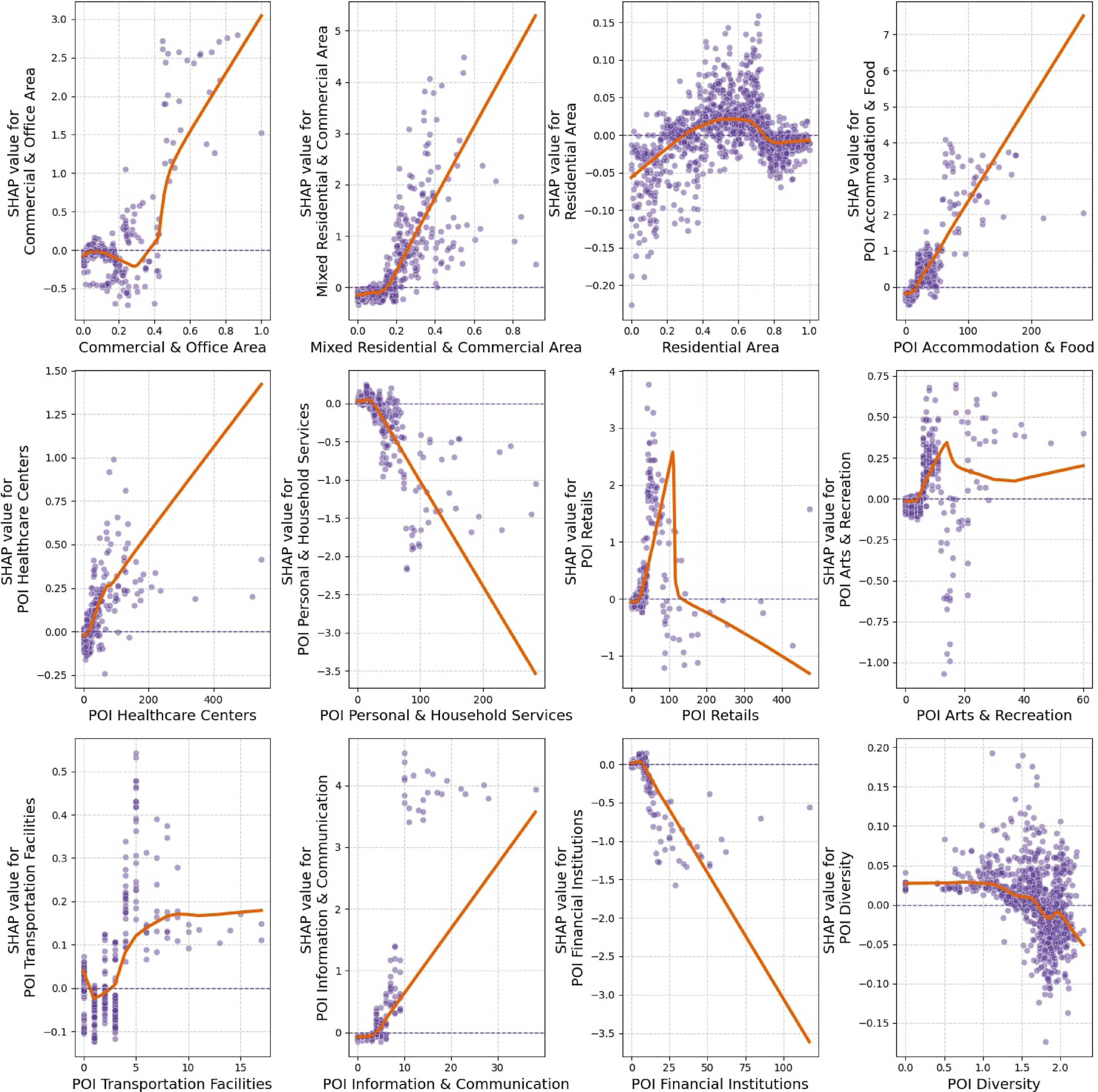
Analysis of nonlinear relationships between environmental factors and homelessness

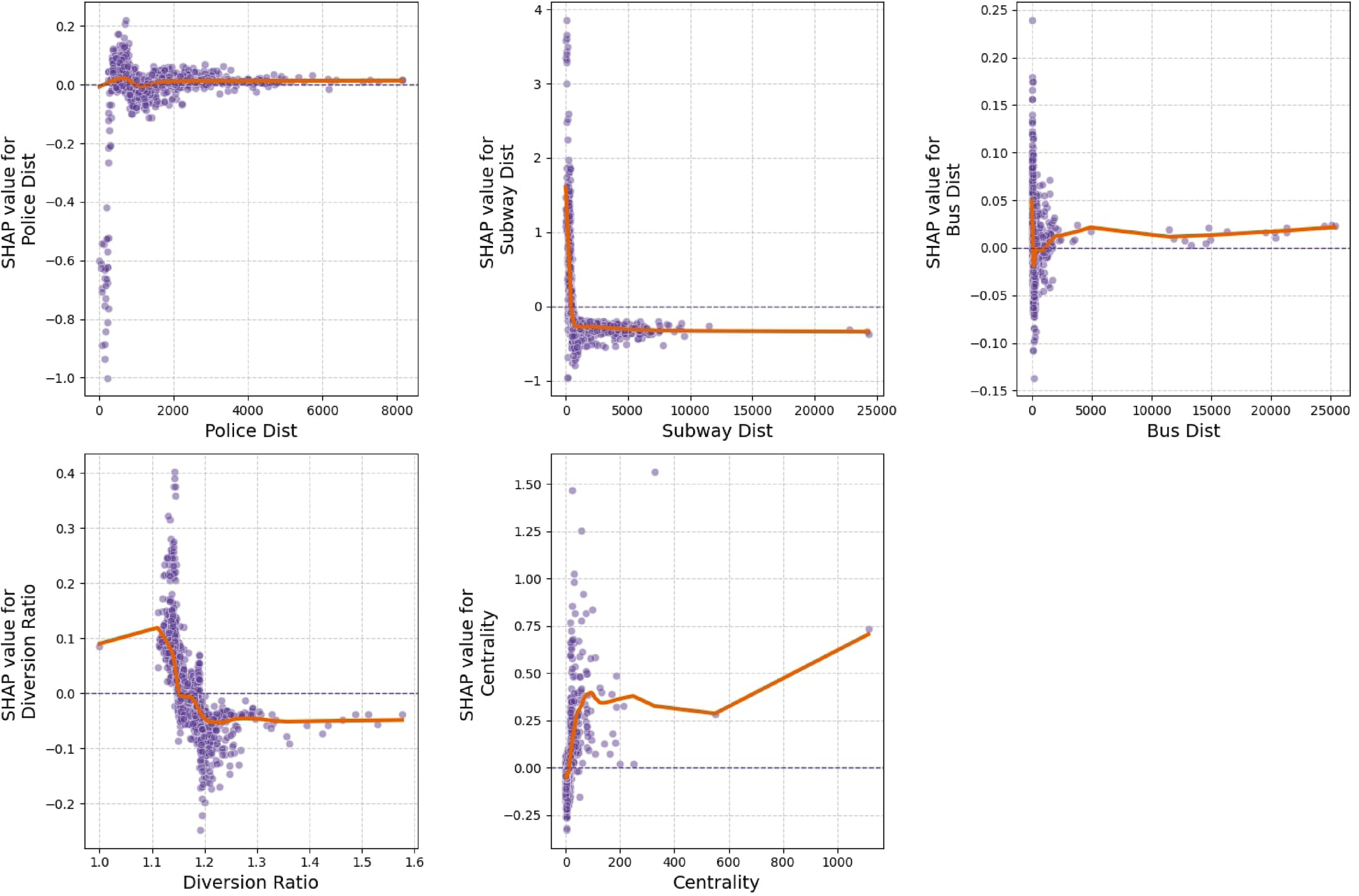
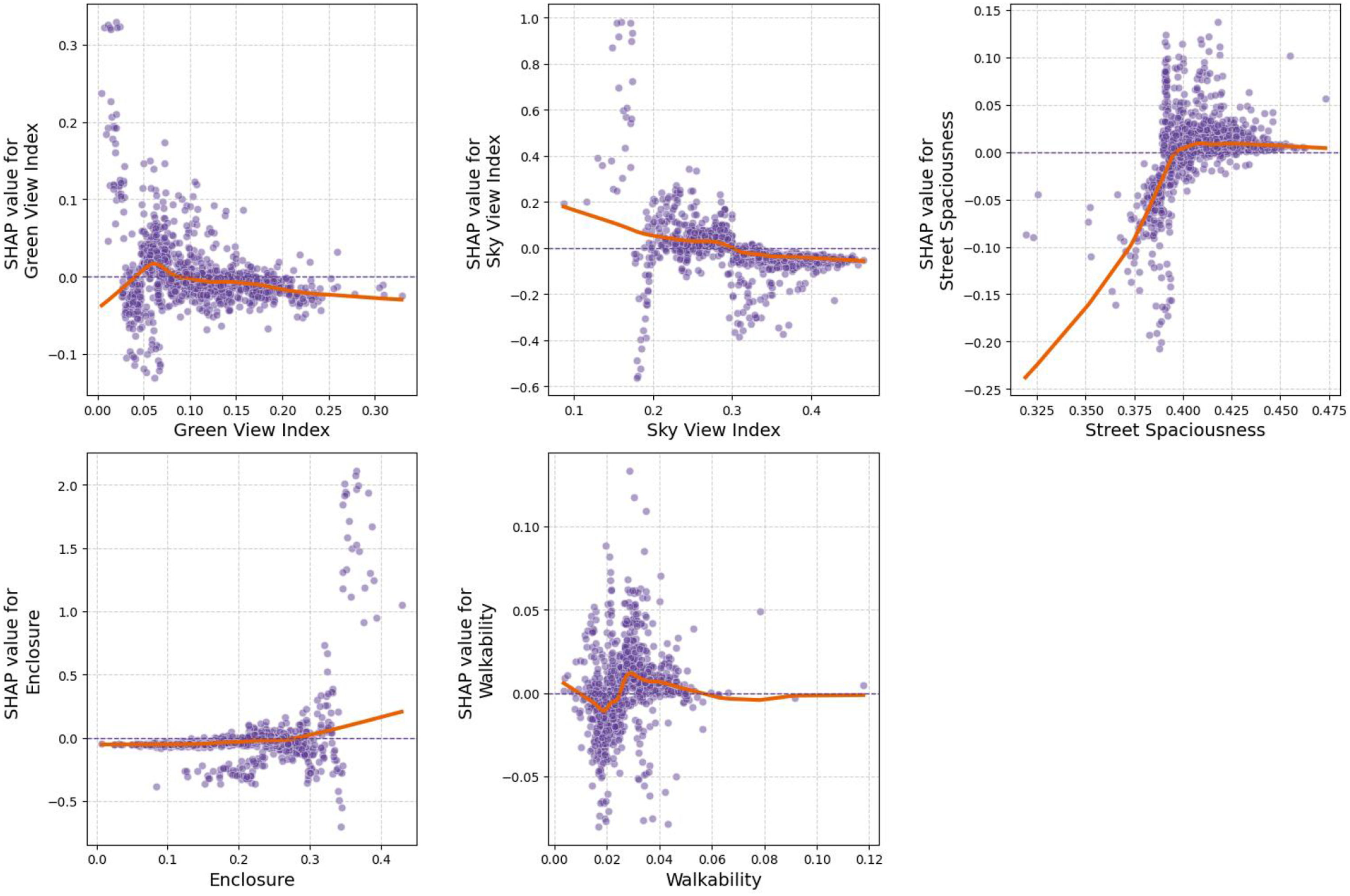
We utilize the Local Dependence Plots (LDPs) to visualize the SHAP values of variables. As shown in Figure 7, we investigated the nonlinear patterns and accurate threshold effects.

(1) Socioeconomic variables. The nonlinear relationships with socioeconomic indicators are shown in Figure 7. Variables such as population density, education level, median rent, household value, Gini index, and felony crime exhibit positive associations with reported homelessness. These associations tend to strengthen beyond certain thresholds, specifically, when population density exceeds 300 people/km², median rent surpasses $1,750, the Gini index exceeds 0.53, or felony crime density exceeds 5 incidence/km². These patterns are consistent with previous findings that areas facing greater economic inequality, housing market stress, or neighborhood instability may experience elevated homelessness incidence. The relationship between median income and homelessness appears reversed U-shaped: homelessness is relatively lower in both low-income (<$70,000) and high-income (>$175,000) areas, and higher in middle-income areas. This may reflect spatial mismatches where homelessness becomes more visible or clustered in neighborhoods facing gentrification, affordability stress, or transitional socioeconomic dynamics. The observed crime density patterns also align with the feature importance seen in Figure 6, reinforcing the spatial co-location between reported crime and homelessness, although causal interpretation remains complex.

(2) Built environment. As shown in Figure 8, reported homelessness incidence is more prevalent in census tracts with greater proportions of mixed residential and commercial land use (over 18%) and commercial/office areas (over 40%). This pattern may indicate a tendency for unhoused individuals to cluster in areas with more foot traffic, service access, or public visibility, rather than suggesting that land use directly causes homelessness. In contrast, predominantly residential areas show relatively stable associations with lower incidence. For POIs, higher numbers of personal and household services, retail businesses, and financial institutions are associated with lower homelessness incidence. These areas may offer greater surveillance or commercial control that limits informal sheltering. On the other hand, greater presence of accommodation and food services, healthcare centers, arts and recreation, and information and communication services shows positive associations with homelessness. These patterns likely reflect the concentration of social service infrastructure or amenity-based clustering rather than direct causal pathways. Lastly, POI diversity shows minimal association with homelessness, suggesting that overall land use mixture is less influential than specific functions or clustering patterns.

(3) Urban transportation. As illustrated in Figure 9, proximity to subway and bus stations demonstrates a nonlinear association with reported homelessness. Within approximately 1000 m, homelessness incidence appears elevated, potentially reflecting the clustering of unhoused individuals near high-access transit hubs. Beyond this threshold, SHAP values decline and stabilize, suggesting diminished relevance at greater distances. These patterns likely reflect post-homelessness settlement behaviors rather than causal effects. The centrality index, which reflects street network connectivity, also shows a positive association with homelessness. This may indicate that highly connected areas offer greater movement opportunities or public visibility for unhoused populations. In contrast, the diversion ratio, which represents street network complexity shows a threshold effect at 1.2. Below this value, homelessness incidence is slightly elevated, possibly reflecting less monitored or fragmented areas, while beyond 1.2, the association turns negative, suggesting lower clustering in more secluded or hard-to-navigate areas. Regarding proximity to police stations, we observe a small decrease in homelessness incidence within the first 500 m. This may reflect deterrence effects or enforcement activity near law enforcement infrastructure. However, this effect flattens out beyond this threshold, suggesting limited spatial influence at larger distances.

(4) Urban landscape. As shown in Figure 10, Both the GVI and SVI show modest negative SHAP values beyond certain thresholds, suggesting a weak inverse association with homelessness. For GVI, the effect becomes more stable and slightly negative after approximately 8%, while SVI’s impact turns increasingly negative beyond 30%. However, these associations may reflect broader urban morphology rather than direct causal mechanisms. For instance, areas with higher GVI and SVI may correspond to lower-density or suburban settings, which typically experience lower visibility of homelessness or may enforce more restrictive public space policies (Neild and Rose, 2018). This interpretation aligns with prior studies noting exclusionary dynamics in highly managed public green spaces. Enclosure and street spaciousness both exhibit positive associations with homelessness when their respective values exceed 0.27 and 0.40. These indicators reflect denser built environments, which may correspond with more heavily urbanized areas where homelessness is both more prevalent and more visible. This suggests a spatial correlation between urban form and where unhoused individuals are reported, rather than a causal effect of enclosure itself. The relationship between walkability and homelessness is more ambiguous, with a weak nonlinear pattern that fluctuates around zero. This may reflect the complex role walkable environments play in shaping public space use, human activity, and visibility. Overall, these urban landscape indicators appear to act more as contextual correlates than direct causal drivers of homelessness. Future research should further investigate how such features interact with land use, policy enforcement, and population density.

Figure 7.

Nonlinear relationships between homeless incidence and socioeconomic features.

Figure 8.

Nonlinear relationships between homeless incidence and built environment.

Figure 9.

Nonlinear relationships between homeless incidence and urban transportation.

Figure 10.

Nonlinear relationships between homeless incidence and urban landscape.

Discussion

Comprehensive analysis of nonlinear relationships

The feature importance rankings varied across location types. For total homelessness, subway distance emerged as the most influential factor, aligning with the high number of reports associated with subway stations (Figure 4). This reflects patterns observed in previous studies, which show that unhoused individuals often seek shelter in or near public transit hubs due to their accessibility, relative safety, and shelter from the elements (Chan et al., 2014; Ding et al., 2022; Loukaitou-Sideris et al., 2020). Other consistently high-ranking features include accommodation and food service POIs, mixed residential and commercial land use, and felony crime density, suggesting the relevance of both built environment and socioeconomic conditions.

In commercial areas, information and communication POIs had the highest importance score, a finding that resonates with research highlighting the growing importance of digital access for unhoused populations. As noted in prior qualitative studies, access to mobile connectivity is essential for navigating public services, staying socially connected, and securing employment opportunities (Goodwin-Smith and Myatt, 2013; Humphry, 2014). However, access to these services remains uneven even in city centers (Humphry and Pihl, 2016), which may exacerbate exclusion in digitally underserved commercial zones. In residential areas, variables such as felony crime, population density, and median income were more pronounced. While the positive correlation between crime and homelessness supports literature that associates neighborhood instability with increased displacement (Ee and Zhang, 2022), the role of population density is more complex. Denser areas may offer greater access to social services and opportunities but could also reflect areas with higher visibility or reporting of homelessness.

The LDPs provided further insight into nonlinear associations and threshold effects. For instance, median income showed a reversed U-shaped relationship with homelessness, with elevated risk in middle-income tracts. This aligns with survey-based research that identifies gentrification and displacement pressures as particularly acute in moderately affluent neighborhoods, where housing costs rise but social safety nets may be insufficient (Byrne et al., 2021; Shelton et al., 2009). Median rent exhibited a clear threshold effect: below $1,800, its influence on homelessness was minimal or negative, but above that point, risk increased sharply—supporting the well-documented link between rent burden and housing precarity (Wetzstein, 2017).

Similarly, urban transportation indicators, such as centrality and subway proximity, showed positive associations with homelessness when accessibility was high. This supports earlier findings that central urban areas and well-connected transit hubs tend to attract homeless individuals seeking proximity to vital services (Jocoy and Del Casino Jr., 2010; Lee et al., 2003). However, it is important to interpret these findings cautiously. These factors likely reflect where homelessness is more visible or reported, rather than serving as direct causes.

Finally, urban landscape indicators such as sky view index, green view index, and enclosure revealed weak-to-moderate associations with homelessness. While greater openness (e.g., higher sky view) and vegetation (e.g., higher GVI) were associated with lower homelessness in some areas, this may reflect broader neighborhood typologies, such as lower-density, higher-income districts rather than a direct mitigating effect of these visual features. Without stronger theoretical or qualitative backing, it would be speculative to claim that increasing green space directly reduces homelessness. Indeed, as previous studies note, parks and open areas are often sites of exclusionary policies (e.g., anti-camping laws) that deter rather than support homeless populations (Amster, 2003; Doherty et al., 2008; Speer and Goldfischer, 2020).

In summary, our results emphasize the spatial concentration and contextual visibility of homelessness rather than simple causal pathways. They underscore the need for nuanced, place-specific strategies that consider the broader social and physical environments in which homelessness occurs.

Policy implications

The results from our feature importance and nonlinear analysis can support the identification of areas with elevated homelessness risk, providing data-driven guidance for targeted interventions and resource allocation. Rather than implying direct causality, our findings point to spatial and environmental conditions that correlate with higher concentrations of homelessness and may reflect underlying vulnerabilities or service needs.

For instance, high importance and threshold patterns in features such as median rent, felony crime, and income inequality reinforce the need to address structural socioeconomic drivers, including housing affordability and neighborhood stability. Policies aimed at preserving affordable housing stock, regulating speculative rent increases, and expanding housing-first programs remain central to reducing homelessness risk.

Regarding built environment variables, results suggest that mixed-use and commercial areas with higher accessibility and service density are more likely to see visible homelessness. These findings could inform the co-location of support services—such as drop-in centers, hygiene facilities, or mobile outreach units—within high-accessibility zones where unhoused individuals are already concentrated, ensuring better alignment of services with population needs.

On the urban landscape side, while variables like green view index and sky openness are associated with lower homelessness incidence in certain contexts, we caution against overgeneralizing these findings. Rather than assuming green space directly reduces homelessness, planners should focus on creating inclusive, accessible public spaces that avoid hostile design and support rest, shade, and dignity especially in areas with limited shelter availability. Initiatives like pocket parks, street trees, and community gardens may be most effective when embedded within broader equity and housing strategies (Cui et al., 2024; Dong et al., 2024, 2025; Middle et al., 2014).

Furthermore, the high importance of information and communication POIs in commercial zones reflects the role of digital access in navigating homelessness. Policymakers should consider expanding public WiFi infrastructure, digital literacy support, and access to mobile charging stations, particularly in areas where homeless individuals congregate. Digital exclusion remains a major barrier to accessing services, employment, and community support.

In sum, addressing homelessness requires an integrated policy approach that combines economic, environmental, and spatial strategies. Tackling root causes, such as housing unaffordability and neighborhood inequity while improving environmental conditions and urban design can contribute to more inclusive, sustainable cities. Governments have both a moral imperative and a practical interest in reducing homelessness, as doing so improves public health, reduces pressure on emergency services, and enhances community resilience.

Limitations and future directions

Despite its contributions, this study has several limitations. First, as a case study focused on NYC, the findings may not be generalizable to other cities with different social, economic, and cultural contexts. Future research should apply this analytical framework to other cities or countries to provide comparative insights into urban homelessness across diverse settings. Additionally, we used census tracts as the primary spatial unit, which may introduce the Modifiable Area Unit Problem (MAUP) (Javanmard et al., 2023). Future studies should explore the impact of different spatial units, such as buffers or census blocks, to assess the robustness of the findings.

Second, the homelessness data used in this study was derived from citizen-reported incidents through the NYC 311 Service Request system. While this provided a large dataset, the data is static and does not capture the dynamic nature of homelessness. Future research should incorporate more dynamic data collection methods, such as real-time tracking through a combination of citizen reports, shelter records, and outreach initiatives. Mobile location data, with appropriate privacy safeguards, could also offer insights into the movement patterns of homeless populations, providing a more comprehensive dataset for analysis.

Third, we acknowledge that our classification of homelessness locations may introduce ambiguity, particularly concerning the distinction between “Street” and other categories. Streets often intersect with commercial and residential areas, making it difficult to ensure that incidents classified as occurring on streets are entirely separate from those in adjacent land-use types. While our spatial data is based on reported coordinates, there is an inherent limitation in verifying whether the recorded location precisely reflects where the incident occurred. Future research should explore alternative classification methods, such as integrating land-use data or clustering techniques, to refine spatial accuracy and improve the interpretation of homelessness distribution.

Additionally, this study employed street-level imagery from Google Street View, primarily vehicle-based, which may inadequately represent certain areas, such as narrow streets or residential neighborhoods, particularly when images are taken from wider avenues (Kim et al., 2021). This methodological limitation warrants acknowledgment, as it may impact the representation and sensitivity of visual urban features within our analysis. Future research could incorporate complementary datasets, such as pedestrian-collected imagery or drone-based visual data, to better capture areas less accessible by vehicles and address this gap.

Finally, while we covered several urban factors, this study did not account for others, such as weather conditions, transient population dynamics, or specific city policies, which could significantly influence homelessness. Additionally, we did not incorporate a temporal analysis, which could reveal how homelessness patterns change over time. Future research should include these variables and analyze the temporal dimension to better understand the dynamic nature of homelessness and its relationship with urban policies, seasonal variations, and population shifts.

Conclusion

Using multi-source urban big data, this study conducted a census tract-level analysis across New York City to investigate the nonlinear associations between urban environmental factors and the incidence of homelessness. By employing a Light Gradient Boosting Machine (LightGBM) model in conjunction with SHapley Additive exPlanations (SHAP), we ensured both strong predictive performance and transparent interpretation of feature effects. Our results reveal three major findings: (1) Feature importance varies by location type. For example, in commercial areas, the prevalence of information and communication POIs was most predictive of homelessness, while in residential areas, factors such as felony crime and median income played more substantial roles. (2) Socioeconomic and built environment factors dominate. Variables related to income, housing cost, crime, and land use consistently exhibited higher predictive importance than transportation or urban landscape indicators. Unlike prior studies that relied on linear models or limited-scale surveys, this study systematically compares multiple environmental dimensions using interpretable machine learning across over 1700 spatial units. (3) Nonlinear and threshold effects are common. Homelessness incidence shows rapid increases beyond specific thresholds—for instance, where median rent exceeds $1800 or the Gini index rises above 0.53 highlighting potential tipping points for targeted interventions. By uncovering key environmental correlates and their threshold effects, this study provides valuable empirical evidence for designing spatially sensitive, equity-driven policy responses. While the study does not assert causal mechanisms, it offers a robust data-driven framework to guide future research and policymaking in the pursuit of more inclusive and sustainable urban environments.

Footnotes

Declaration of conflicting interests

The author(s) declared no potential conflicts of interest with respect to the research, authorship, and/or publication of this article.

Funding

The author(s) disclosed receipt of the following financial support for the research, authorship, and/or publication of this article: This work was supported by the National Science Foundation, USA (No. 2314709).

ORCID iDs

Shengao Yi

Wei Tu

Xiaojiang Li

Data Availability Statement

Data will be made available on request.

Shengao Yi is a Ph.D. student at Department of City and Regional Planning, University of Pennsylvania, concentrating on environmental planning and urban analytics. He is also a research fellow at Penn Institute for Urban Research and associate fellow at Leonard Davis Institute of Health Economics, University of Pennsylvania, aiming to combine Science, Data, and Design together to tackle the pressing urban challenges through the collaboration with communities. His research focuses on AI for environmental planning, optimization and design, micro-scale urban analytics, and GeoAI. Aspiring to an academic career, he is dedicated to addressing socio-environmental challenges by developing innovative AI-driven approaches to mitigate urban heat exposure, optimize green infrastructure and enhance urban resilience.

Wei Tu is a distinguished professor and chair at Department of Urban Informatics, School of Architecture and Urban Planning, Shenzhen University, China. He obtained the Ph.D. from State Key Laboratory of Information Engineering in Surveying, Mapping and Remote Sensing, Wuhan University, China. His research interests focus on the urban informatics, including data-driven human activity-mobility (i.e., taxi GPS, bus GPS, smart card data, social media data, mobile phone data, etc.), multi-source geospatial data fusion, and smart applications in the cities worldwide.

Tianhong Zhao is an Assistant Professor at the School of Big Data and Internet, Shenzhen Technology University. He obtained his Ph.D. from the School of Architecture and Urban Planning at Shenzhen University, specializing in Urban Informatics. He was a visiting scholar at the Urban Analytics Lab, National University of Singapore. His research focuses on the GeoAI, Spatiotemporal Prediction and Intelligent Optimization Algorithm.

Xiaojiang Li is a tenure-track Assistant Professor at Department of City and Regional Planning, University of Pennsylvania. He is also the co-founder of Biometeors. He was a Postdoctoral Fellow at MIT Senseable City Lab. His research focuses on developing and applying geospatial analyses and data-driven approaches in the domain of urban studies. He has proposed to use Google Street View for urban environment studies and developed the Treepedia project, which aims to map street greenery for cities around the world. He is working on HeatExpo using artificial intelligence, remote sensing, urban microclimate modeling, and urban analytics to investigate the different vulnerabilities to climate change across different neighborhoods in the U.S. He is also working on using human trace data to study human activities and investigate the connection between urban environments and human activities.

Yatao Zhang is a doctoral student at the Mobility Information Engineering lab at ETH Zurich and the Future Resilient Systems at the Singapore-ETH centre. He received the B.S. degree in geographical information science from Sun Yat-sen University and the M.S. degree in geographical information science from Wuhan University. His research interests lie in context-based spatiotemporal analysis, geospatial big data mining, and traffic forcasting.

Donghang Li is a graduate student at MIT, pursing the Master of Science in Transportation (MST) degree. Before joining MIT, he obtained dual Bachelor's degrees in Economics and Urban Planning from Peking University. His research interests lie at the intersection of artificial intelligence, causal inference, and urban computing. He is currently working as a research assistant at the Singapore-MIT Alliance for Research and Technology (SMART), focusing on the social and economic impacts of artificial intelligence.

Joseph Rodriguez is a Ph.D. candidate at Northeastern Univeristy, working with Prof. Haris Koutsopoulos on the application of AI/ML methods for real-time control of fixed and flexible transit systems, including its implementability on the field. His experience includes leading the testing of control strategies in a bus route in Chicago.

Yifei Sun is a research assistant at The Hong Kong University of Science and Technology (Guangzhou). She is a master graduate of the Urban Spatial Analytics program at University of Pennsylvania. Prior to that, she obtained her bachelor's degree in GIS from Northwest A&F University. Her research interests include GeoAI, human mobility, and urban informatics.

References

Adadi

Berrada

(2018) Peeking inside the black-box: a survey on explainable artificial intelligence (xai). IEEE Access 6: 52138–52160.

Amore

Baker

Howden-Chapman

(2011) The ethos definition and classification of homelessness: an analysis. European Journal of Homelessness 5(2).

Amster

(2003) Patterns of exclusion: sanitizing space, criminalizing homelessness. Social Justice 30(91): 195–221.

Anguche

(2024) Homelessness in the United States and its effects on the economy. Available at SSRN 5092765.

Aron

(2002) The 1996 national survey of homeless assistance providers and clients: faith-based and secular non-profit programs.

Barton

Gibbons

(2017) A stop too far: how does public transportation concentration influence neighbourhood median household income? Urban Studies 54(2): 538–554.

Batterham

(2019) Defining “at-risk of homelessness”: Re-connecting causes, mechanisms and risk. Housing, Theory and Society 36(1): 1–24.

Bensken

Krieger

Berg

, et al. (2021) Health status and chronic disease burden of the homeless population: an analysis of two decades of multi-institutional electronic medical records. Journal of Health Care for the Poor and Underserved 32(3): 1619–1634.

Berk

MacDonald

(2010) Policing the homeless: an evaluation of efforts to reduce homeless-related crime. Criminology & Public Policy 9(4): 813–840.

10.

Bocarejo

Portilla

Velásquez

, et al. (2014) An innovative transit system and its impact on low income users: the case of the metrocable in medellín. Journal of Transport Geography 39: 49–61.

11.

Bogar

Beyer

(2016) Green space, violence, and crime: a systematic review. Trauma, Violence, & Abuse 17(2): 160–171.

12.

Bradford

Lozano-Rojas

(2024) Higher rates of homelessness are associated with increases in mortality from accidental drug and alcohol poisonings: study examines the association between homelessness and accidental drug and alcohol mortality. Health Affairs 43(2): 242–249.

13.

Breiman

(2001) Random forests. Machine Learning 45: 5–32.

14.

Byrne

Henwood

Orlando

(2021) A rising tide drowns unstable boats: how inequality creates homelessness. The Annals of the American Academy of Political and Social Science 693(1): 28–45.

15.

Canham

Donovan

Rose

, et al. (2023) Transportation needs and mobility patterns of persons experiencing homelessness following shelter decentralization. Evaluation and Program Planning 99: 102306. DOI: 10.1016/j.evalprogplan.2023.102306.

16.

Caruana

Lou

Gehrke

, et al. (2015) Intelligible models for healthcare: predicting pneumonia risk and hospital 30-day readmission. In: Proceedings of the 21th ACM SIGKDD International Conference on Knowledge Discovery and Data Mining. New York: Association for Computing Machinery, 1721–1730.

17.

Chan

Gopal

Helfrich

(2014) Accessibility patterns and community integration among previously homeless adults: a geographic information systems (gis) approach. Social Science & Medicine 120: 142–152.

18.

Chen

Guestrin

(2016) Xgboost: a scalable tree boosting system. In: Proceedings of the 22nd Acm Sigkdd International Conference on Knowledge Discovery and Data Mining. New York: Association for Computing Machinery, 785–794.

19.

Chen

Zhu

Papandreou

, et al. (2018) Encoder-decoder with atrous separable convolution for semantic image segmentation. In: Proceedings of the European Conference on Computer Vision (ECCV). Berlin, Germany: Springer, 801–818.

20.

Chen

, et al. (2024) Lcz-based city-wide solar radiation potential analysis by coupling physical modeling, machine learning, and 3d buildings. Computers, Environment and Urban Systems 113: 102176.

21.

Cleveland

(2020) Homelessness and inequality. The American Journal of Economics and Sociology 79(2): 559–590.

22.

Constantinescu

Brasoveanu

(2020) The homelessness phenomenon in the contemporary society. Revista Universitara de Sociologie 16(2): 393–401.

23.

Cordts

Omran

Ramos

, et al. (2016) The cityscapes dataset for semantic urban scene understanding. In: Proceedings of the IEEE Conference on Computer Vision and Pattern Recognition. Piscataway: IEEE, 3213–3223.

24.

Cui

Tan

, et al. (2024) Effective or useless? assessing the impact of park entrance addition policy on green space services from the 15-min city perspective. Journal of Cleaner Production 467: 142951.

25.

Currie

Patterson

Moniruzzaman

, et al. (2014) Examining the relationship between health-related need and the receipt of care by participants experiencing homelessness and mental illness. BMC Health Services Research 14: 1–10.

26.

De Nadai

Letouzé

, et al. (2020) Socio-economic, built environment, and mobility conditions associated with crime: a study of multiple cities. Scientific Reports 10(1): 1–12.

27.

Deb

Smith

(2021) Application of random forest and shap tree explainer in exploring spatial (in) justice to aid urban planning. ISPRS International Journal of Geo-Information 10(9): 629.

28.

DePastino

(2003) Citizen Hobo: How a Century of Homelessness Shaped America. Chicago: University of Chicago Press.

29.

Derrien

Cerveny

Bratman

, et al. (2023) Unsheltered homelessness in public natural areas across an urban-to-wildland system: institutional perspectives. Society & Natural Resources 36(8): 947–969.

30.

Ding

Loukaitou-Sideris

Wasserman

(2022) Homelessness on public transit: a review of problems and responses. Transport Reviews 42(2): 134–156.

31.

Dobson

(2022) Complex needs in homelessness practice: a review of ‘new markets of vulnerability. Housing Studies 37(7): 1147–1173.

32.

Doherty

Busch-Geertsema

Karpuskiene

, et al. (2008) Homelessness and exclusion: regulating public space in european cities. Surveillance and Society 5(3): 290–314.

33.

Dong

Yang

, et al. (2024) Planning for green infrastructure by integrating multi-driver: ranking priority based on accessibility equity. Sustainable Cities and Society 114: 105767.

34.

Dong

, et al. (2025) Adaptive ranking of specific tree species for targeted green infrastructure intervention in response to urban hazards. Urban Forestry and Urban Greening 107: 128776.

35.

Doshi-Velez

Kim

(2017) Towards a rigorous science of interpretable machine learning. arXiv preprint arXiv:1702.08608.

36.

Zhang

(2022) Homelessness and crime in neighborhoods. Crime & Delinquency 70: 00111287221140835.

37.

Fischer

Shinn

Shrout

, et al. (2008) Homelessness, mental illness, and criminal activity: examining patterns over time. American Journal of Community Psychology 42: 251–265.

38.

Folsom

Hawthorne

Lindamer

, et al. (2005) Prevalence and risk factors for homelessness and utilization of mental health services among 10,340 patients with serious mental illness in a large public mental health system. American Journal of Psychiatry 162(2): 370–376.

39.

Ford

Cramb

Farah

(2014) Oral health impacts and quality of life in an urban homeless population. Australian Dental Journal 59(2): 234–239.

40.

Foster

Kleit

(2015) The changing relationship between housing and inequality, 1980–2010. Housing Policy Debate 25(1): 16–40.

41.

Fowle

(2022) Racialized homelessness: a review of historical and contemporary causes of racial disparities in homelessness. Housing Policy Debate 32(6): 940–967.

42.

Frank

Sallis

Conway

, et al. (2006) Many pathways from land use to health: associations between neighborhood walkability and active transportation, body mass index, and air quality. Journal of the American Planning Association 72(1): 75–87.

43.

Friedman

(2001) Greedy function approximation: a gradient boosting machine. Annals of Statistics 29: 1189–1232.

44.

Fusaro

Levy

Shaefer

(2018) Racial and ethnic disparities in the lifetime prevalence of homelessness in the United States. Demography 55: 2119–2128.

45.

Goodling

(2020) Intersecting hazards, intersectional identities: a baseline critical environmental justice analysis of us homelessness. Environment and Planning E: Nature and Space 3(3): 833–856.

46.

Goodwin-Smith

Myatt

(2013) Homelessness and the role of information technology in staying connected.

47.

Hatami

Rahman

Nikparvar

, et al. (2023) Non-linear associations between the urban built environment and commuting modal split: a random forest approach and shap evaluation. IEEE Access 11: 12649–12662.

48.

Zhang

Ren

, et al. (2016) Deep residual learning for image recognition. In: Proceedings of the IEEE Conference on Computer Vision and Pattern Recognition. Piscataway: IEEE, 770–778.

49.

Hennigan

(2017) House broken: homelessness, housing first, and neoliberal poverty governance. Urban Geography 38(9): 1418–1440.

50.

Hill

(1994) The public policy issue of homelessness: a review and synthesis of existing research. Journal of Business Research 30(1): 5–12.

51.

Homeless

CFT

(2019) Basic facts about homelessness: New york city.

52.

Humphry

(2014) Homeless and connected: mobile phones and the internet in the lives of homeless Australians.

53.

Humphry

Pihl

(2016) Making connections: young people, homelessness and digital access in the city. Melbourne: Young and Well Cooperative Research Centre.

54.

Hwang

Weaver

Aubry

, et al. (2011) Hospital costs and length of stay among homeless patients admitted to medical, surgical, and psychiatric services. Medical care 49(4): 350–354.

55.

Jarvis

(2015) Individual determinants of homelessness: a descriptive approach. Journal of Housing Economics 30: 23–32.

56.

Javanmard

Lee

Kim

, et al. (2023) The impacts of the modifiable areal unit problem (maup) on social equity analysis of public transit reliability. Journal of Transport Geography 106: 103500.

57.

Wang

Lyu

, et al. (2022) Understanding cycling distance according to the prediction of the xgboost and the interpretation of shap: a non-linear and interaction effect analysis. Journal of Transport Geography 103: 103414.

58.

Jocoy

Casino

(2010) Homelessness, travel behavior, and the politics of transportation mobilities in long beach, California. Environment and Planning A 42(8): 1943–1963.

59.

Meng

Finley

, et al. (2017) Lightgbm: a highly efficient gradient boosting decision tree. Advances in Neural Information Processing Systems 30: 3149–3157.

60.

Kelling

Bratton

(1997) Declining crime rates: insiders’ views of the new york city story. Journal of Criminal Law and Criminology 88: 1217.

61.

Kiesler

(1991) Homelessness and public policy priorities. American Psychologist 46(11): 1245–1252.

62.

Kim

(2022) Explainable heat-related mortality with random forest and shapley additive explanations (shap) models. Sustainable Cities and Society 79: 103677.

63.

Kim

Lee

(2023) Nonlinear relationships and interaction effects of an urban environment on crime incidence: application of urban big data and an interpretable machine learning method. Sustainable Cities and Society 91: 104419.

64.

Kim

Lee

Hipp

, et al. (2021) Decoding urban landscapes: google street view and measurement sensitivity. Computers, Environment and Urban Systems 88: 101626.

65.

Klaassen

Hoogland

Van Pelt

(2022) Economic impact and implications of shelter investments. In: Shelter, Settlement & Development. Milton Park: Routledge, 35–59.

66.

Koprowska

Kronenberg

Kuźma

, et al. (2020) Condemned to green? accessibility and attractiveness of urban green spaces to people experiencing homelessness. Geoforum 113: 1–13.

67.

Kuhn

Culhane

(1998) Applying cluster analysis to test a typology of homelessness by pattern of shelter utilization: results from the analysis of administrative data. American Journal of Community Psychology 26(2): 207–232.

68.

Lee

Price-Spratlen

Kanan

(2003) Determinants of homelessness in metropolitan areas. Journal of Urban Affairs 25(3): 335–356.

69.

Lewer

Aldridge

Menezes

, et al. (2019) Health-related quality of life and prevalence of six chronic diseases in homeless and housed people: a cross-sectional study in london and birmingham, england. BMJ Open 9(4): e025192.

70.

Zhang

, et al. (2015) Assessing street-level urban greenery using google street view and a modified green view index. Urban Forestry and Urban Greening 14(3): 675–685.

71.

Lin

Kim

Wada

, et al. (2022) Unemployment, homelessness, and other societal outcomes in patients with schizophrenia: a real-world retrospective cohort study of the United States veterans health administration database: societal burden of schizophrenia among us veterans. BMC Psychiatry 22(1): 458.

72.

Loukaitou-Sideris

Wasserman

Caro

, et al. (2020) Homelessness in transit environments volume i: findings from a survey of public transit operators.

73.

Lundberg

Lee

(2017) A unified approach to interpreting model predictions. Advances in Neural Information Processing Systems 30: 4768–4777.

74.

, et al. (2021) Measuring human perceptions of streetscapes to better inform urban renewal: a perspective of scene semantic parsing. Cities 110: 103086.

75.

Mago

Morden

Fritz

, et al. (2013) Analyzing the impact of social factors on homelessness: a fuzzy cognitive map approach. BMC Medical Informatics and Decision Making 13(1): 1–19.

76.

Majumder

Roy

Bose

, et al. (2023) Multiscale gis based-model to assess urban social vulnerability and associated risk: evidence from 146 urban centers of eastern India. Sustainable Cities and Society 96: 104692.

77.

Meng

Zacharias

(2021) Street morphology and travel by dockless shared bicycles in beijing, China. International journal of sustainable transportation 15(10): 788–798.

78.

Middle

Dzidic

Buckley

, et al. (2014) Integrating community gardens into public parks: an innovative approach for providing ecosystem services in urban areas. Urban Forestry and Urban Greening 13(4): 638–645.

79.

Murphy

(2019) Transportation and homelessness: a systematic review. Journal of Social Distress and the Homeless 28(2): 96–105.

80.

Neild

Rose

(2018) An exploration of unsheltered homelessness management on an urban riparian corridor. People, Place and Policy Online 12(2): 84–98.

81.

Nishio

Horita

Sado

, et al. (2017) Causes of homelessness prevalence: R elationship between homelessness and disability. Psychiatry and Clinical Neurosciences 71(3): 180–188.

82.

Onapa

Sharpley

Bitsika

, et al. (2022) The physical and mental health effects of housing homeless people: a systematic review. Health and Social Care in the Community 30(2): 448–468.

83.

O’flaherty

(1996) Making Room: The Economics of Homelessness. Cambridge: Harvard University Press.

84.

Parrott

Huslage

Cronley

(2022) Educational equity: a scoping review of the state of literature exploring educational outcomes and correlates for children experiencing homelessness. Children and Youth Services Review 143: 106673.

85.

Quigley

Raphael

(2001) The economics of homelessness: the evidence from north America. European Journal of Housing Policy 1(3): 323–336.

86.

Racionero-Plaza

Vidu

Diez-Palomar

, et al. (2021) Overcoming limitations for research during the covid-19 pandemic via the communicative methodology: the case of homelessness during the Spanish home confinement. International Journal of Qualitative Methods 20: 16094069211050164.

87.

Ranasinghe

Valverde

(2006) Governing homelessness through land-use: a sociolegal study of the toronto shelter zoning by-law. The Canadian Journal of Sociology 31: 325–349.

88.

Ribeiro

Singh

Guestrin

(2016) “Why should i trust you?” explaining the predictions of any classifier. In: Proceedings of the 22nd ACM SIGKDD International Conference on Knowledge Discovery and Data Mining. New York: Association for Computing Machinery, 1135–1144.

89.

Rose

(2019) Unsheltered homelessness in urban parks: perspectives on environment, health, and justice in salt lake city, Utah. Environmental Justice 12(1): 12–16.

90.

Rossi

(1991) Down and Out in America: The Origins of Homelessness. Chicago: University of Chicago Press.

91.

Rudin

(2019) Stop explaining black box machine learning models for high stakes decisions and use interpretable models instead. Nature Machine Intelligence 1(5): 206–215.

92.

Salit

Kuhn

Hartz

, et al. (1998) Hospitalization costs associated with homelessness in new york city. New England Journal of Medicine 338(24): 1734–1740.

93.

Schütz

(2016) Homelessness and addiction: causes, consequences and interventions. Current Treatment Options in Psychiatry 3: 306–313.

94.

Sewell

(1993) The Shape of the city: Toronto struggles with Modern Planning. Toronto: University of Toronto Press.

95.

Sharam

Hulse

(2014) Understanding the nexus between poverty and homelessness: relational poverty analysis of families experiencing homelessness in Australia. Housing, Theory and Society 31(3): 294–309.

96.

Shelton

Taylor

Bonner

, et al. (2009) Risk factors for homelessness: evidence from a population-based study. Psychiatric Services 60(4): 465–472.

97.

Speck

(2018) Walkable City Rules: 101 Steps to Making Better Places. Washington: Island Press.

98.

Speer

Goldfischer

(2020) The city is not innocent: homelessness and the value of urban parks. Capitalism Nature Socialism 31(3): 24–41.

99.

Stansfield

Semenza

(2023) Urban housing affordability, economic disadvantage and racial disparities in gun violence: a neighbourhood analysis in four us cities. British Journal of Criminology 63(1): 59–77.

100.

Tam

Zlotnick

Robertson

(2003) Longitudinal perspective: adverse childhood events, substance use, and labor force participation among homeless adults. The American Journal of Drug and Alcohol Abuse 29(4): 829–846.

101.

Van

Vanos

Middel

, et al. (2024) Concurrent heat and air pollution exposures among people experiencing homelessness. Environmental health perspectives 132(1): 015003.

102.

VanBerlo

Ross

Rivard

, et al. (2021) Interpretable machine learning approaches to prediction of chronic homelessness. Engineering Applications of Artificial Intelligence 102: 104243.

103.

Vangeest

Johnson

(2002) Substance abuse and homelessness: direct or indirect effects? Annals of Epidemiology 12(7): 455–461.

104.

Vaswani

Shazeer

Parmar

, et al. (2017) Attention is all you need. Advances in Neural Information Processing Systems 30.

105.

Walters

Businelle

Suchting

, et al. (2021) Using machine learning to identify predictors of imminent drinking and create tailored messages for at-risk drinkers experiencing homelessness. Journal of Substance Abuse Treatment 127: 108417.

106.

Wang

Meng

, et al. (2022) Assessing street space quality using street view imagery and function-driven method: the case of xiamen, China. ISPRS International Journal of Geo-Information 11(5): 282.

107.

Wang

Sun

, et al. (2025) Exploring the associations between street-view green space quantity and quality, and influenza in guangzhou, China through machine learning and spatial regression: a socio-economic equity perspective. Environment and Planning B: Urban Analytics and City Science 23998083241312272.

108.

Wetzstein

(2017) The global urban housing affordability crisis. Urban Studies 54(14): 3159–3177.

109.

Willison

(2021) Ungoverned and Out of Sight: Public Health and the Political Crisis of Homelessness in the United States. Oxford: Oxford University Press.

110.

Wusinich

Bond

Nathanson

, et al. (2019) “if you’re gonna help me, help me”: barriers to housing among unsheltered homeless adults. Evaluation and Program Planning 76: 101673.

111.

Xiao

Liu

, et al. (2021) Nonlinear and synergistic effects of tod on urban vibrancy: applying local explanations for gradient boosting decision tree. Sustainable Cities and Society 72: 103063.

112.

Wang

, et al. (2024) Interpretable spatial machine learning insights into urban sanitation challenges: a case study of human feces distribution in san francisco. Sustainable Cities and Society 113: 105695.

113.

, et al. (2025) Assessing the differential impact of vegetated and built-up areas on heat exposure environment: a case study of los angeles. Building and Environment 271: 112538.

114.

Yue

Zhuang

Yeh

, et al. (2017) Measurements of poi-based mixed use and their relationships with neighbourhood vibrancy. International Journal of Geographical Information Science 31(4): 658–675.

115.

Zhu

Yuan

, et al. (2023) Neoliberalization and inequality: disparities in access to affordable housing in urban Canada 1981–2016. Housing Studies 38(10): 1860–1887.

116.

Zlotnick

Robertson

Tam

(2002) Substance use and labor force participation among homeless adults. The American Journal of Drug and Alcohol Abuse 28(1): 37–53.

Uncovering nonlinear urban factors of homelessness: Evidence from New York City using interpretable machine learning

Abstract

Keywords

Introduction

Related works

Socioeconomic and built environment determinants of urban homelessness

Applications of interpretable machine learning methods

Materials and methods

Study area and datasets

Study area

Data sources

Model constructions

Dependent variable

Independent variables

Regression models

Model interpretation with SHAP

Results

Model evaluation results

Analysis of features importance in different locations

Analysis of nonlinear relationships between environmental factors and homelessness

Discussion

Comprehensive analysis of nonlinear relationships

Policy implications

Limitations and future directions

Conclusion

Footnotes

Declaration of conflicting interests

Funding

ORCID iDs

Data Availability Statement

References