Sage Journals: Discover world-class research

Abstract

Income inequality, which refers to the uneven distribution of income in a population, has been linked to many societal problems, including crime. Although environmental criminology theories, such as rational choice theory, suggest a positive association between income inequality and crime, previous empirical studies have reported divergent results based on different crime types, statistical models, and spatial units of analysis. This study employs non-spatial and spatial regression models using frequentist and Bayesian modelling frameworks to explore the impacts of within-area and across-area income inequality on five types of major crimes in the City of Toronto at the census tract and dissemination area scales. The use of spatial regression models improves the model fit in both frequentist and Bayesian frameworks. The Bayesian shared component model, which accounts for the interactions between different types of crimes, further enhances model performance. Results obtained from the best-fitting frequentist and Bayesian models are inconsistent but do not conflict in terms of the relationship between crime and income inequality, where within-area income inequality generally increases major crime rates, while across-area income inequality has varying effects dependent on crime type and spatial scale. The discrepancies between spatial scales are a manifestation of the modifiable areal unit problem (MAUP).

Keywords

Income inequality crime spatial regression Bayesian modelling modifiable areal unit problem

Introduction

Income inequality, which refers to the uneven distribution of income in a population, is a global concern, especially in urban cores and areas of high population density. Research has identified the detrimental effects of income inequality on many dimensions of society, including population health, economic growth, education systems, social trust, and crime control (Dabla-Norris et al., 2015; Kawachi and Kennedy, 1999; Pickett and Wilkinson, 2010). Among these social issues, studying crime as a direct threat to public safety is of particular interest. The links between income inequality and crime are supported by multiple criminology theories. For example, rational choice theory indicates that income inequality increases the relative benefits of illegal activities compared to legal activities and hence motivates the poorer population to commit crimes (Cornish and Clarke, 1986). As crime occurrences are usually not randomly distributed across space, research on the income inequality-crime relationship can aid the understanding of crime patterns and strengthen crime prediction and prevention.

Empirical studies about the income inequality-crime relationship have been conducted in different regions around the world and divergent results have been reported. Many studies have demonstrated a positive association between income inequality and crime (e.g. Costantini et al., 2018; Enamorado et al., 2016; Fajnzylber et al., 2002; Kennedy et al., 1998). On the contrary, some studies have shown that the effects of income inequality on crime are insignificant, spurious, or negative (e.g. Allen, 1996; Dong et al., 2020; Kang, 2016; Neumayer, 2005). The inconsistencies in previous empirical study results are likely driven by different research contexts. For example, analyses of different crime types (e.g. violent crime vs property crime) may produce different outcomes, which is supported by studies that have explored the relationships between income inequality and multiple types of crimes (e.g. Bhorat et al., 2017; Choe, 2008; Kelly, 2000).

Furthermore, the choice of statistical modelling approaches may affect the analytical results and conclusions. Various statistical methods have been employed in previous studies of income inequality and crime, including bivariate correlation (e.g. Pickett et al., 2005), non-spatial regression (e.g. Coccia, 2017; Neumayer, 2005), and spatial regression (e.g. Metz and Burdina, 2018; Scorzafave and Soares, 2009). In recent crime research, Bayesian modelling has become popular, and it offers various advantages compared to the traditional frequentist approaches, such as the incorporation of prior knowledge (e.g. Law et al., 2014; Quick et al., 2018). However, Bayesian methods have not been widely applied to the analysis of the income inequality-crime relationship.

Finally, the spatial scales at which crime and income inequality are quantified may also influence analytical results and conclusions. This is known as the modifiable areal unit problem (MAUP), which recognizes that data is usually arbitrarily aggregated in geographic studies and different data aggregation units may lead to different parameter estimates in multivariate analysis (Fotheringham and Wong, 1991; Openshaw, 1984). Although many spatial units, ranging from the country scale to the finest census scale, have been adopted in previous studies of the income inequality-crime relationship, limited research has examined the MAUP effects by analyzing multiple spatial scales. Furthermore, some studies suggest that when smaller spatial units are used, income inequality may be better captured by across-area measures that quantify the income differences between neighbouring areas, rather than using traditional within-area measures that represent income distribution in each individual area (Metz and Burdina, 2018; Wang and Arnold 2008).

To validate the aforementioned hypotheses regarding the causes of the divergent empirical results about the income inequality-crime relationship, there is a need to conduct a study that examines multiple crime types, statistical models, and spatial scales simultaneously on the same data source and study area. This study aims to contribute to better understanding the income inequality-crime relationship and its sensitivity to crime type, statistical modelling approach, and spatial scale. While some previous studies have recognized the importance of these factors, the extent of their influence on analysis results and underlying conclusions remains unclear. This study addresses this gap by testing these factors via empirical analyses based on a consistent dataset from the City of Toronto, Canada. Non-spatial and spatial regression models using frequentist and Bayesian approaches are applied to quantify the impacts of within-area and across-area income inequality on the crime rates of five major crimes (assault, robbery, auto theft, break and enter, and theft over $5000) at the census tract and dissemination area levels. Results from different models and different spatial scales are compared in this research. This study does not seek to identify a universally suitable model or spatial scale for analyzing the income inequality-crime relationship for each crime type. Instead, it aims to inform researchers about how different analysis settings can influence results and their interpretations. This could potentially guide future research in improving the robustness of analyses, ultimately contributing to more accurate policy recommendations. By examining the associations between income inequality and major crimes, this study also seeks to strengthen the understanding of spatial crime patterns within Toronto neighbourhoods, which will potentially aid in informing local crime prevention and control practices.

Literature review

Theoretical links between income inequality and crime

Rational choice theory, social disorganization theory, strain theory, and routine activity theory are frequently cited environmental criminology theories, which explain how crime patterns are determined by different physical or social characteristics, including income inequality. Rational choice theory states that people voluntarily and knowingly choose to violate laws after making rational considerations of the costs and benefits of both legal and illegal activities (Becker, 1968; Cornish and Clarke, 1986). When there is significant income inequality, low-income individuals may believe that directly making benefits from high-income individuals via criminal offences may bring about higher returns than retaining normal market activities (Chiu and Madden 1998; McCarthy 2002). Nevertheless, when targeting affluent individuals involves great risks of punishment due to enhanced self-protection and policing in their areas, offenders may opt to victimize the poor (Kang, 2016).

Social disorganization theory links adverse community characteristics, such as low socioeconomic status (low income, low education attainments, etc.), residential instability, and ethnic heterogeneity, with high levels of violence and crime (Bursik and Grasmick, 1999; Elliott et al., 1996; Sampson and Groves, 1989). While this theory has conventionally focused on individual neighbourhoods, more recent studies have found that community characteristics in surrounding areas can also influence crime (Chamberlain and Hipp, 2015; Stucky et al., 2016). Sampson et al. (1997) argue that the intervening variable between these community characteristics and crime rates is collective efficacy, which reflects social cohesion and the shared attitudes among community members towards social control. Income inequality, as part of unfavourable socioeconomic status, participates in the social disorganization process by increasing social distance and reducing interactions among community members (Hipp, 2007). Inequality may also reduce trust and heighten stress in social interactions, thereby weakening community participation and social cohesion (Wilkinson and Pickett, 2017).

Strain theory highlights the impacts of social environments on individual mental status. Individuals who are in a struggle to achieve socially valued goals (e.g. monetary success) tend to experience strains and frustrations, which can further lead to more negative thoughts and ultimately motivate them to commit criminal offences (Cohen 1955; Merton 1938). Agnew (1992) emphasizes the role of the social comparison process referenced in this theory. Research has found that comparing an individual’s income to wealthier neighbours can create a sense of unfairness and diminish life satisfaction, particularly in regions with higher levels of inequality (Cheung and Lucas, 2016; Oshio et al., 2011). Increased income inequality at the community level can heighten strains and distress among lower-income individuals, potentially leading to higher rates of criminal behaviour (Vilalta-Perdomo et al., 2022).

Routine activity theory states that a crime incident requires the presence of a suitable target, a potential offender, and the lack of guardianship at the same location and time (Cohen and Felson, 1979). As a result, criminal offending tends to cluster in areas with abundant crime opportunities (e.g. business areas without video surveillance). Widening income inequality could change the crime opportunity structure in multiple directions. For example, when the income gap is large, more affluent residents can become more attractive targets to the poor, but they might also be able to afford better security measures (i.e. guardianship) against potential offenders (Madero-Hernandez and Fisher, 2012). Moreover, potential offenders from lower-income neighbourhoods may target individuals in nearby affluent areas, since their routine activity spaces extend across multiple neighbourhoods, indicating that the economic conditions of nearby areas can influence each other’s crime rates (Metz and Burdina, 2018; Ramos and Melo, 2022; Stucky et al., 2016).

Frequentist and Bayesian approaches in crime research

Frequentist regression models have been widely applied in the analysis of risk factors for crime, where classical models, such as the ordinary least squares (OLS) model, assume no spatial autocorrelation in crime. Spatial autocorrelation refers to the systematic variation in a variable across space, including positive spatial autocorrelation, where similar values tend to cluster, and negative spatial autocorrelation, where neighbouring values tend to be dissimilar (Haining, 1990). When spatial autocorrelation exists, spatial regression models, instead of classical regression models that assume spatial randomness, should be used to prevent biased results while analyzing crime in cross-sectional geographic units (Anselin, 1988; Anselin et al., 2000).

Although the use of frequentist regression is commonly accepted in crime research, some studies have instead suggested the use of Bayesian regression approaches. Frequentist inference and Bayesian inference are two statistical inferential paradigms to make estimates of parameters while modelling real-world processes. In contrast to frequentist statistics, which considers parameters as unknown constants, Bayesian statistics considers parameters as random variables and provides probability statements of the parameter values by combining prior knowledge and the observed data based on Bayes’ theorem (Bolstad and Curran, 2016).

It has become common practice to use smaller spatial units of analysis in crime research, since smaller units tend to have more homogenous environmental conditions (Weisburd et al., 2009). Law et al. (2014) argue that Bayesian regression is a preferable approach in small-area crime analysis for several reasons: (1) Bayesian models in hierarchical structures can integrate crime information from different sources; (2) Bayesian methods are able to fit more complex spatial models due to the use of Markov Chain Monte Carlo (MCMC) simulation; (3) while frequentist spatial regression is designed for analyzing continuous crime rates, Bayesian regression can model discrete crime counts; (4) the Bayesian approach has a better handle of the small number problem, where minor changes in crime counts could significantly impact the crime rates and lead to unstable parameter estimates. Furthermore, the Bayesian approach provides a convenient way of modelling the interactions between multiple types of crimes, which can potentially improve model performance (e.g. Law et al., 2020; Liu and Zhu, 2017; Quick et al., 2018). Despite these advantages, Bayesian modelling does not necessarily produce more accurate results compared to frequentist modelling. Wakefield (2013) states that issues such as parameter interpretation and model misspecification are much more important than the inferential approach adopted and suggests that the frequentist and Bayesian approaches can be applied to the same data to compare the results and to attain a better understanding of the associations between variables.

Study area and data sources

The study area is the City of Toronto, the core of the largest metropolitan area in Canada. With a population of over 2.7 million from diverse demographics, Toronto has experienced increasing inequality and polarization during the past few decades (Walks, 2014). Although Toronto is known as a safe city compared to most major metropolitans in the world, the crime severity index, which indicates both the amount and seriousness of police-reported crime, has increased for five consecutive years since 2014 (Statistics Canada, 2020a).

To investigate the effects of spatial scale, this study adopts two small census geographic units, census tracts (CT) and dissemination areas (DA). There are 572 CTs and 3702 DAs in Toronto and all DAs are wholly nested within CTs. 5 CTs and 67 DAs within the study area did not have complete data or spatial neighbours (for the purpose of spatial modelling) and were therefore excluded from this study. Figure 1 illustrates the boundaries of CTs and DAs in the study area and the excluded areas are marked.

Figure 1.

Census Tracts (CTs, left) and Dissemination Areas (DAs, right) in the City of Toronto.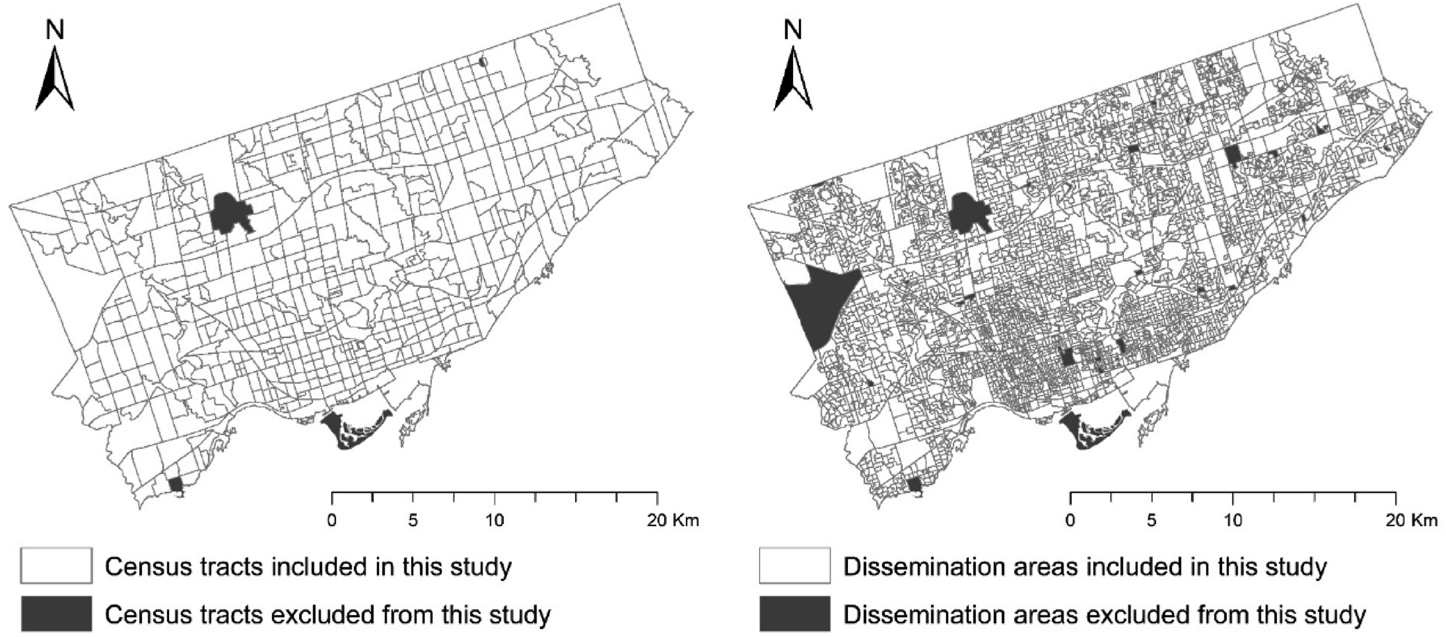

Two data sources were used in this study. The major crime indicators data retrieved from the Toronto Police Public Safety Data Portal (Toronto Police Service, 2020) was used to represent major crime occurrences in Toronto. This data records the dates and locations of incidents of five major crime types (assault, robbery, auto theft, break and enter, and theft over $5000) between 2014 and 2019. All other data used in this study, including census boundaries, income data, and other sociodemographic data, were extracted from the 2016 census of Canada (Statistics Canada, 2020b).

Regression modelling

Frequentist models

Three frequentist models were adopted to assess the relationship between income inequality and crime. Model (1) is an OLS model, which estimates the natural log of crime rate ( $Y_{k i}$ ) of crime type $k$ in area $i$ as the sum of an intercept term ( $α_{k}$ ), the product of the explanatory variable vector ( $X_{i}$ ) and the regression coefficient vector ( $β_{k}$ ), and a random error ( $e_{k i}$ ). The crime rate was calculated as one plus the crime count, divided by the population (one was added to avoid zeros in the log transformation). This model assumes spatial randomness and was used as a benchmark frequentist model.

\log (Y_{k i}) = α_{k} + X_{i} β_{k} + e_{k i}

(1)

To account for spatial autocorrelation, two frequentist spatial models were considered. Model (2), known as the spatial lag model, includes a spatial autoregressive coefficient ( $ρ_{k}$ ) to assess the effect of the spatial lag term for the dependent variable ( ${W y}_{k i}$ ). Model (3), known as the spatial error model, includes a spatial autoregressive multiplier ( $λ_{k}$ ) to assess the effect of the spatial lag term for the error ( ${W e}_{k i}$ ). The spatial lag of a value is the average value of its spatial neighbours, and spatial neighbours in this study are defined as different areas that share at least one vertex or edge (i.e. queen contiguity). The spatial lag model accounts for the influence of the dependent variable on the values of the dependent variable in neighbouring areas, while the spatial error model accounts for the spatial dependence in the error term (Ward and Gleditsch, 2008).

\log (Y_{k i}) = {ρ_{k} {W y}_{k i} + α}_{k} + X_{i} β_{k} + e_{k i}

(2)

\log (Y_{k i}) = α_{k} + X_{i} β_{k} + {W e}_{k i} λ_{k} + e_{k i}

(3)

Based on Anselin (1988, 2005), this study used Lagrange Multiplier (LM) test statistics to detect model misspecification caused by spatial autocorrelation and aid in deciding which spatial regression model to use. Since the underlying processes of crime are complicated, this study recognizes that the LM test result is not a universal standard for the choice of spatial model. Therefore, both spatial models were tested for all crime types at both spatial scales regardless of the LM test diagnostics. We found that the choice between Model (2) and Model (3) did not significantly affect the main conclusions drawn about the income inequality-crime relationship.

Bayesian models

Hierarchical regression models were employed to examine the relationship between income inequality and crime in the Bayesian framework. Instead of calculating crime rates, the crime count ( $O_{k i}$ ) of crime type $k$ in area $i$ was modelled using a Poisson distribution with a mean equal to the product of the population ( $p_{i}$ ) in area $i$ and the crime rate ( $μ_{k i}$ ) of crime type $k$ in area $i$ . In Model (4), the natural log of crime rate is expressed as the sum of an intercept term ( $α_{k}$ ), the product of the explanatory variable vector ( $X_{i}$ ) and the regression coefficient vector ( $β_{k}$ ), and a spatial random error term ( $e_{k i}$ ). Similar to frequentist regression, this non-spatial model was used as a benchmark Bayesian method.

\log (μ_{k i}) = α_{k} + X_{i} β_{k} + e_{k i}

(4)

In Bayesian modelling, priors are required for unknown parameters. For each crime type, $α_{k}$ was given a uniform distribution; every regression coefficient in $β_{k}$ was given a normal distribution with the mean equal to 0 and the variance equal to 1000; $e_{k i}$ was given a normal distribution with the mean equal to 0 and the variance equal to $σ_{e k}^{2}$ . The reciprocal of $σ_{e k}^{2}$ was modelled in a commonly used distribution of $G a m m a (0.5, 0.0005)$ . The use of such vague priors for the intercept and regression coefficients is common practice adopted in crime modelling when there is no genuine prior knowledge (e.g. Law and Haining, 2004; Liu and Zhu, 2017; Quick et al., 2018).

To account for spatial autocorrelation, Model (5) adds a structured spatial error term ( $s_{k i}$ ), which has an intrinsic conditional autoregressive (ICAR) prior. The ICAR model assumes positive spatial autocorrelation and $s_{k i}$ is normally distributed with the mean equal to the spatial lag of $s_{k i}$ and the variance equal to $σ_{s k}^{2} / n_{i}$ , where $n_{i}$ is the number of neighbouring areas to area $i$ . The reciprocal of $σ_{s k}^{2}$ was given the same Gamma distribution as $σ_{e k}^{2}$ . This model is based on the well-known BYM (Besag-York-Mollié) structure proposed by Besag et al. (1991).

\log (μ_{k i}) = α_{k} + X_{i} β_{k} + (s_{k i} + e_{k i})

(5)

Considering the possible interactions between different crime types, Model (6) includes an additional spatial shared component ( $l_{k} ϕ_{i}$ ), where $ϕ_{i}$ is the spatial effect in area $i$ shared by all crime types and $l_{k}$ is the factor loading of crime type $k$ for $ϕ_{i}$ . This model assumes that all crime types are positively associated, but every crime type has a unique association with the shared spatial effects. For each crime type, $l_{k}$ was given a positive half-normal prior distribution with the mean equal to 0 and the variance equal to 1000. This prior restricts the five types of crime to be positively associated with each other. $ϕ_{i}$ was given an ICAR distribution with the variance fixed to 1. Since this model involves factor analysis, without constraints, there can be multiple equivalent solutions that prevent the MCMC chains from convergence. The fixed variance and the positive factor loadings act as an identifiability constraint in the priors and guarantee a unique solution to $l_{k}$ and $ϕ_{i}$ (Tzala and Best, 2008).

\log (μ_{k i}) = α_{k} + X_{i} β_{k} + (s_{k i} + e_{k i}) + l_{k} ϕ_{i}

(6)

Regression variables

Five types of major crimes (assault, robbery, auto theft, break and enter, and theft over $5000) were used as dependent variables in regression modelling. Because crime data in small areas tends to experience high volatility, crime counts were calculated over a 5-year period (2015–2019) in this research. Significantly positive spatial autocorrelation was identified in each type of crime using global Moran’s I. Similar spatial patterns were observed across different types of crime using local Moran’s I statistics, and bivariate correlation analyses revealed that all types of crime are positively associated with one another. These findings imply the importance to account for spatial autocorrelation in crime and the associations between crime types in regression modelling. Detailed results of the spatial autocorrelation and bivariate correlation tests are provided in the Supplemental Material.

Two income inequality variables (within-area and across-area income inequality) were considered as explanatory variables. The first variable was the Gini coefficient, a commonly used metric of inequality in the literature. Higher Gini values indicate higher levels of income inequality within individual areas. The second variable captures a different dimension of income inequality at the small-area level, where residents may travel across spatial units for work, recreation, etc. Based on routine activity theory, potential offenders can be motivated by the economic disparities between neighbouring areas and commit crimes outside their areas of residence, which makes it important to account for across-area income inequality (Metz and Burdina, 2018; Wang and Arnold, 2008). Based on Metz and Burdina (2018), the across-area income inequality variable (% richer than the poorest Neighbour) was calculated as the percentage difference between an area’s median income and the minimum median income in its neighbouring areas.

Four control variables were also included as explanatory variable. Corresponding to some major risk factors for crime indicated by criminology theories, the control variables were residential instability, ethnic heterogeneity, low education attainments, and population density. Detailed information about the regression variables, including calculation methods and descriptive statistics for all variables, control variable selection, and maps of income inequality variables, are provided in the Regression Variables Section of the Supplemental Materials.

Results

Frequentist regression was implemented in GeoDa (Anselin et al., 2010). Table 1 shows the regression coefficient estimates of the two income inequality variables obtained from the frequentist models. For each OLS regression, the LM-lag statistic and LM-error statistic were computed and found to be significant. This indicates that the assumption of spatial randomness in OLS regression was violated, and the OLS results could be biased. The robust LM statistics were further compared based on the methodology described by Anselin (2005). If the robust LM-lag statistic was more significant, the spatial lag model (Model (2)) was adopted; if the robust LM-error statistic was more significant, the spatial error model (Model (3)) was adopted. The commonly used p-value of 0.05 was used to determine significant associations. Akaike Information Criterion (AIC) was calculated to assess model fit, where models with smaller AIC values are considered to be better (Akaike, 1973). The spatial model (Model (2) or Model (3)) always has a smaller AIC value than the OLS model (Model (1)). Complete frequentist regression results with all regression coefficient estimates and AIC values are provided in the Supplemental Materials (Tables S3 and S4).

Table 1.

Frequentist regression results for the income inequality variables (regression coefficients with standard errors in parentheses).

		Assault	Robbery	Auto theft	Break and enter	Theft over $5000
Census tracts
Gini Coefficient	Model (1)	0.029* (0.0081)	0.019* (0.0083)	0.009 (0.0067)	0.043* (0.0065)	0.023* (0.0070)
Gini Coefficient	Model (2) or (3)	0.022* (0.0077)	0.012 (0.0079)	0.004 (0.0071)	0.033* (0.0062)	0.019* (0.0069)
% Richer than the poorest neighbour	Model (1)	0.002* (0.0009)	0.001 (0.0010)	0.002* (0.0008)	0.004* (0.0008)	0.003* (0.0008)
% Richer than the poorest neighbour	Model (2) or (3)	0.001 (0.0009)	0.000 (0.0009)	0.001 (0.0007)	0.003* (0.0007)	0.002* (0.0008)
Dissemination areas
Gini Coefficient	Model (1)	0.022* (0.0030)	0.018* (0.0025)	0.004 (0.0022)	0.025* (0.0024)	0.013* (0.0018)
Gini Coefficient	Model (2) or (3)	0.019* (0.0029)	0.015* (0.0026)	0.005* (0.0023)	0.021* (0.0025)	0.011* (0.0018)
% Richer than the poorest neighbour	Model (1)	0.002* (0.0003)	0.001* (0.0002)	0.001* (0.0002)	0.002* (0.0002)	0.001* (0.0002)
% Richer than the poorest neighbour	Model (2) or (3)	0.001* (0.0002)	0.001* (0.0002)	0.001* (0.0002)	0.002* (0.0002)	0.001* (0.0002)

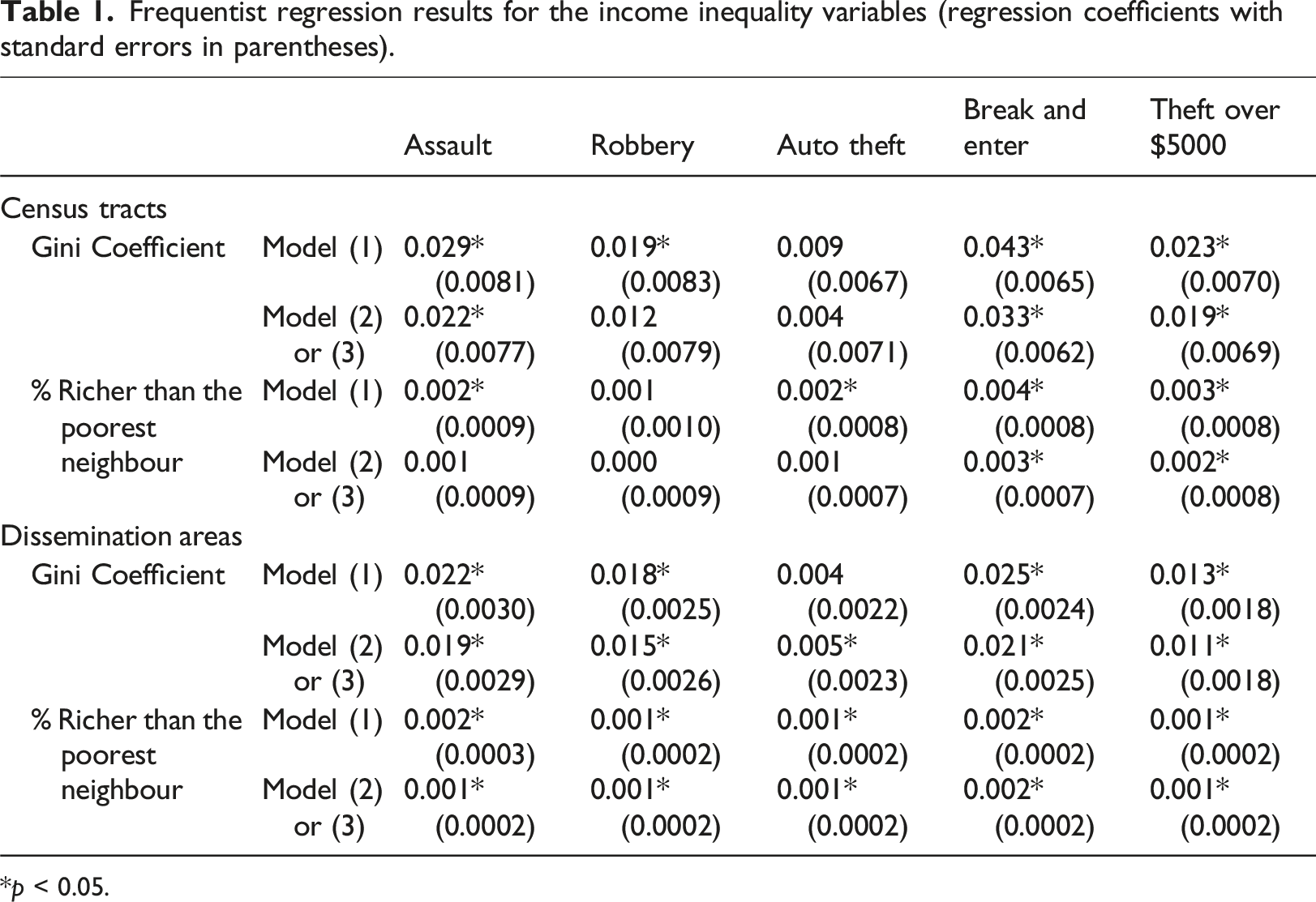
*p < 0.05.

Bayesian regression analysis was implemented in WinBUGS (Spiegelhalter et al., 2003). For each model run, two parallel MCMC chains with different initial values were used. Convergence was reached by 50,000 iterations for each model and posterior statistics were obtained from additional 50,000 iterations after convergence. The Monte Carlo error for each parameter was smaller than 5% of its posterior standard deviation, indicating that the number of iterations to generate the posterior distribution was sufficient (Spiegelhalter et al., 2003). Table 2 shows the posterior means of the two income inequality variables. A regression coefficient is considered to be significant when it is consistently positive or negative at the 95% credible interval (CI) of the posterior distribution. The Deviance Information Criterion (DIC) was used to evaluate the Bayesian models, where a smaller value indicates a better model fit (Spiegelhalter et al., 2002). The non-spatial model (Model (4)) always has the largest DIC values, and the shared spatial component model (Model (6)) always has the smallest DIC values. All crime types had to be included in one model in Model (6), which produced a single DIC value at each spatial scale. In order to compare DIC values between models, for the other two models, the five types of crimes were also included in one model instead of five separate models. Nevertheless, these two models were also tested for each crime type separately. The regression results remain the same and for every crime type, while Model (5) always resulted in smaller DIC values than Model (4). Complete results that include the posterior means and 95% CIs of all regression coefficients and the DIC values of all models are provided in Supplemental Materials (Tables S5–S7).

Table 2.

Bayesian regression results for the income inequality variables (regression coefficients with 95% credible intervals in parentheses).

		Assault	Robbery	Auto theft	Break and enter	Theft over $5000
Census tracts
Gini Coefficient	Model (4)	0.029* (0.014, 0.044)	0.022* (0.005, 0.038)	0.007 (−0.006, 0.020)	0.043* (0.031, 0.055)	0.027* (0.011, 0.042)
	Model (5)	0.005 (−0.011, 0.021)	0.001 (−0.018, 0.019)	−0.002 (−0.016, 0.011)	0.021* (0.008, 0.034)	0.011 (−0.007, 0.028)
	Model (6)	−0.003 (−0.017, 0.010)	−0.007 (−0.023, 0.008)	−0.009 (−0.021, 0.003)	0.015* (0.004, 0.026)	0.000 (−0.015, 0.015)
% Richer than the poorest neighbour	Model (4)	0.002* (0.000, 0.004)	0.001 (−0.001, 0.003)	0.002* (0.000, 0.003)	0.004* (0.002, 0.005)	0.003* (0.001, 0.005)
	Model (5)	−0.001 (−0.003, 0.001)	−0.002 (−0.004, 0.000)	0.001 (−0.000, 0.002)	0.001 (−0.000, 0.003)	0.002 (−0.000, 0.003)
	Model (6)	−0.002* (−0.003,−0.001)	−0.003* (−0.004,−0.001)	0.000 (−0.001, 0.001)	0.001 (−0.001, 0.002)	0.000 (−0.001, 0.002)
Dissemination areas
Gini coefficient	Model (4)	0.026* (0.019, 0.032)	0.029* (0.021, 0.038)	0.003 (−0.003, 0.009)	0.029* (0.024, 0.035)	0.030* (0.022, 0.038)
	Model (5)	0.013* (0.006, 0.019)	0.019* (0.010, 0.028)	0.002 (−0.003, 0.008)	0.014* (0.008, 0.019)	0.015* (0.006, 0.024)
	Model (6)	0.007 (−0.000, 0.014)	0.013* (0.004, 0.022)	0.000 (−0.007, 0.006)	0.010* (0.004, 0.016)	0.010* (0.001, 0.019)
% Richer than the poorest neighbour	Model (4)	0.002* (0.001, 0.002)	0.002* (0.001, 0.003)	0.001* (0.001, 0.002)	0.002* (0.002, 0.002)	0.002* (0.001, 0.003)
	Model (5)	0.001* (0.001, 0.002)	0.001* (0.001, 0.002)	0.001* (0.001, 0.002)	0.001* (0.001, 0.002)	0.002* (0.001, 0.002)
	Model (6)	0.001* (0.000, 0.002)	0.001* (0.000, 0.002)	0.001* (0.001, 0.002)	0.001* (0.001, 0.002)	0.001* (0.001, 0.002)

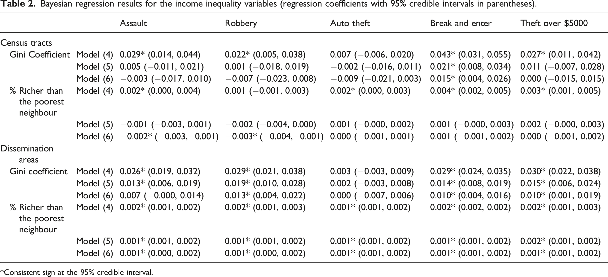
*Consistent sign at the 95% credible interval.

Discussion

Comparing regression results of different models

This research considered five crime types, two income inequality variables, and two spatial scales, resulting in 20 possible links assessed between income inequality and crime. Such links are represented by the regression coefficient estimates obtained from each model, and discrepancies have been observed in the regression coefficient results of different models. In the frequentist results, the Gini coefficient shows a significant positive association with robbery at the CT scale in the OLS model (Model (1)), but this relationship is not significant in the spatial model (Model (2) or (3)). Moreover, the positive association between the Gini coefficient and auto theft at the DA scale is significant in the spatial model, but not in the OLS model. Because of the presence of significant spatial autocorrelation in crime, the OLS model might produce biased results in which some associations could be either underestimated or overestimated (Anselin et al., 1996; Ward and Gleditsch, 2008). The smaller AIC values also imply that the spatial model have an improved goodness of fit compared to the OLS model, suggesting that the spatial model results may be more reliable in assessing the income inequality-crime relationships.

Similar findings can be identified in the Bayesian regression results. In the results of Model (4), 17 of the 20 associations assessed between income inequality and crime are found to be significantly positive. Among these 17 links, 10 and 9 remain significant in Model (5) and Model (6), respectively. Additionally, Model (6) shows two significantly negative associations between % richer than the poorest neighbour and crime, which are not evident in the other models. Based on the DIC values, Model (5), which accounts for spatial autocorrelation in each type of crime, outperforms Model (4), which assumes spatial randomness. Model (6), which includes an additional term to capture the spatial interactions between different types of crimes, has the smallest DIC values. Since similar spatial patterns have been identified in different types of crimes, it is reasonable to conclude that Model (6) is the best-fitting Bayesian model.

Inconsistencies can also be found between the frequentist and Bayesian results. When considering the best-fitting frequentist model (Model (2) or Model (3)) and Bayesian model (Model (6)), discrepancies in regression coefficient estimates could be a result of the contrasting inferential approaches and the different methods to define significance. Furthermore, the inconsistencies could also be caused by the differences in model specifications. First, to adjust for spatial autocorrelation, the frequentist model includes a spatially lagged term (lagged dependent variable or lagged error) while the Bayesian model takes advantage of the MCMC algorithm and uses the ICAR model to represent the structured spatial errors. Second, Model (6) includes a spatial shared component to model the interactions between crime types, which was not applied to the frequentist model. Third, crime rates were directly calculated using crime counts and populations in the frequentist models while the Bayesian method modelled crime counts using Poisson distributions. This results in different interpretations of regression coefficients. In the OLS model, a coefficient represents the change in the log of the crime rate for one unit change in the explanatory variable. However, with a spatially lagged term, the coefficient reflects both direct and indirect effects, complicating its interpretation. In the Bayesian models, the regression coefficient represents the change in the log of the crime count for one unit change in the explanatory variable, adjusted by the population count. Bayesian modelling with Poisson distribution might be a more appropriate method when crime counts are available.

Moreover, since the frequentist and Bayesian models approached the regression coefficient estimates using contrasting methods, the significance levels of the coefficients were defined in different ways. For each regression coefficient in the frequentist model, the p-value, which tested the null hypothesis of no correlation between the dependent variable and the explanatory variable (i.e. the coefficient value is equal to zero) was used to define significance. Alternatively, the significance could be defined by examining whether the 95% confidence interval of the coefficient (i.e. a range of values with a probability of 95% to contain the true value of the coefficient) contained zero. In Bayesian models, a regression coefficient was deemed to be significant when the 95% credible interval did not contain zero. Different from the confidence interval in frequentist modelling, the 95% credible interval is a range of values that cover 95% of the probability in the posterior probability distribution.

Given that Bayesian modelling can properly account for the count data, the small number problem, and the interactions between multiple dependent variables, Bayesian regression models may be preferable compared to frequentist regression for the purposes of this study. However, this does not necessarily mean frequentist modelling should be completely abandoned. While Bayesian models can be more flexible and complicated, the reliability of such models is subject to the prior settings. For example, in Model (6), the priors that assumed positive associations between all types of crimes could be problematic if such associations were untrue. Moreover, while running more complex Bayesian models tend to be computationally intensive and time-consuming, frequentist models provide an efficient way for data analysts or researchers to draw a preliminary conclusion before embarking on further analysis. One can have more confidence in the research conclusions of a study when the results of frequentist and Bayesian methods are consistent and do not differ significantly. In this study, since the results obtained from the best-fitting frequentist and Bayesian models are not conflicting, that is, no association is found significantly positive in one model but significantly negative in the other model, both results are retained and considered when assessing the income inequality-crime relationships.

The income inequality-crime relationship and the issue of spatial scale

Based on the best-fitting frequentist model (Model (2) or Model (3)) and Bayesian model (Model (6)), different impacts of within-area income inequality (Gini coefficient) and across-area income inequality (% richer than the poorest neighbour) on five major crime types have been identified at the CT and DA scales. At the CT scale, there is a strongly positive association between within-area income inequality and break and enter, since the significance of this association is not sensitive to the choice of regression model. Within-area income inequality may also have positive relationships with assault and theft over $5,000, as indicated by the frequentist model results. These positive effects are in agreement with the expectation that income inequality may be a driver of higher crime rates.

For across-area income inequality at the CT scale, the frequentist results highlight the positive impacts of % richer than the poorest neighbour on two property crime types (break and enter and theft over $5000). This matches the findings of Metz and Burdina (2018), who applied similar income inequality measures and indicated that larger income disparities between neighbouring areas may motivate residents from poorer areas to steal from richer areas. On the other hand, the Bayesian results indicate negative impacts of the across-area income inequality measure on two violent crime types (assault and robbery) at the CT level, which means that violent crimes are more likely to occur in poorer CTs than in their richer neighbours. This could be a result of social disorganization, where relatively poor CTs may have worse social cohesion and social control within communities and hence provide more suitable environments for breeding violent behaviour compared to more affluent CTs nearby. Offenders may also prefer to target these poorer CTs after rational consideration, as the risks of punishment could be lower compared to nearby wealthier CTs.

At the DA scale, positive impacts of within-area income inequality on robbery, break and enter, and theft over $5000 are identified in both models and it may also have positive effects on assault and auto theft as indicated by the frequentist spatial model results. The effect of % richer than the poorest neighbour is significantly positive on all crime types in both models at the DA scale. The differences between the CT-level and DA-level results are a manifestation of the scale effect in the MAUP, which concerns the impacts of different spatial resolutions (Fotheringham and Wong, 1991; Openshaw, 1984). When incidents are aggregated into larger spatial units, the crime levels in an area may disproportionately reflect some localized extreme patterns or mask some outlying local patterns (Weisburd et al., 2009). The scale effect is also important when considering the explanatory variables in the regression models, including the two income inequality variables.

Figure 2 demonstrates the MAUP effects in measuring crime rates and income inequality within this study, using a CT from the study area as an example. Assault rates vary significantly across DAs, with eastern DAs showing notably lower rates. When aggregated into CTs, these variations are generalized into a medium crime rate, which masks all the localized patterns. For income inequality, the MAUP effects can be more complex. As shown in the figure, the example CT records a Gini coefficient that is higher than all DA-level Gini coefficients within the CT. This type of discrepancies between scales are not simply explained by the generalization effects of the larger spatial unit. Instead, they involve transformations between across-area and within-area income inequality. The median incomes shown in the figure reveals that the eastern DAs within the example CT have higher-income levels compared to the western DAs, which might be captured by the across-DA income inequality measure. However, when these DAs are aggregated into a CT, the across-DA disparities translate into within-CT inequality, resulting in a high Gini value that is not seen at the DA scale. For across-area income inequality, changes in spatial scale alter both the income measures and the neighbouring areas used for comparison, thereby affecting the resulting values.

Figure 2.

Impacts of aggregation from DAs to CTs on measuring crime rates and income inequality.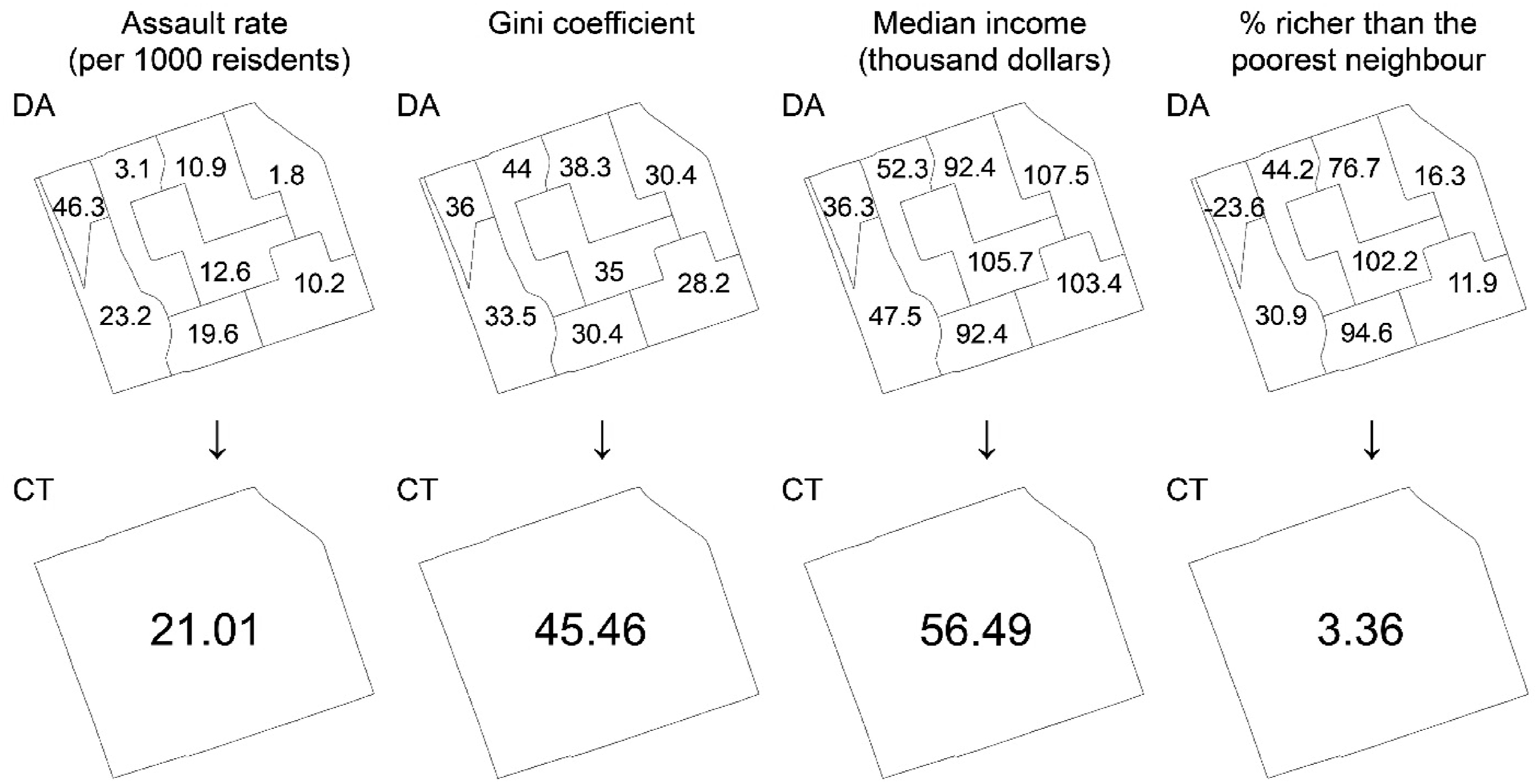

The MAUP effects on both crime rates and income inequality measures collectively contribute to the discrepancies observed in regression results between the two spatial scales. The choice of scale also affects the interpretation of results. For within-area income inequality, the differing findings between the two spatial scales can suggest whether inequality within a CT or within a DA more significantly influences crime. For across-area income inequality, the spatial units not only affect the aggregation of income levels, but also the distance between neighbouring areas. This could explain why the effects of % richer than the poorest neighbour are consistently positive at the DA scale. Since neighbouring DAs are within relatively short distances compared to neighbouring CTs, residents are usually knowledgeable about and able to travel to their nearby DAs. Thus, DAs that are richer than their neighbours may project a sense of inequality to residents in neighbouring DAs and subsequently attract potential criminals of all crime types, who try to ‘level the field’ via illegal means. The DA, as a smaller spatial unit that represents more homogeneous areas and captures detailed local variations, may be preferable for analyzing crime and neighbourhood characteristics (Prouse et al., 2014; Weisburd et al., 2009). Nevertheless, this does not necessarily mean the CT scale has no value. Income inequality is inherently a spatial issue, as it involves comparing the income of different individuals or groups within a specific geographical area. Without sufficient prior knowledge of the spatial scale at which such comparisons are perceived and ultimately influence crime, researchers should always be mindful of the MAUP, conduct sensitivity analyses using various spatial units, and interpret the findings accordingly.

While the CTs and DAs capture different aspects of the relationship between income inequality and crime, different results can be potentially obtained using other spatial units. It is also noteworthy that CTs and DAs may not accurately reflect the ‘true’ neighbourhoods within which daily social interactions are made or how income inequality is perceived. The ‘true’ neighbourhoods may be larger than CTs or smaller than DAs. Even at the same spatial resolution, neighbourhood boundaries may be drawn differently, which reflects the zoning effect of the MAUP (Jelinski and Wu, 1996; Openshaw, 1984). Indeed, there has not been universal agreement on how to define a ‘neighbourhood’ and different residents within a small area could have different perceived neighbourhoods based on their mobility ranges and levels of participation in social activities. Despite the uncertainties in identifying actual neighbourhoods, the use of administrative units such as CT and DA can provide insights that can be easily incorporated into policy and planning decisions related to inequality reduction and crime control in the City of Toronto.

Limitations and future research

This study has several limitations from both data and methodological perspectives. First, the quantification methods of deriving crime counts and crime rates were not ideal. According to Moreau (2019), the crime reporting rate in Canada was only 31% in 2014, meaning that crime counts based on police-reported crime data might have ignored a significant number of unreported crime incidents. Future research could incorporate alternative data sources for crime when available, such as perceived fear of crime based on survey results. Census population counts were used as the denominator for calculating crime rates, similar to many other studies. However, it is recognized that the census population does not account for daytime population movements and hence it cannot accurately represent the at-risk population. Future research could incorporate other datasets when available (e.g. daytime population) and potentially adopt different at-risk populations for different crime types (e.g. using the number of dwellings for break and enter).

Second, the two income inequality measures were constrained by the census data, and they also did not encompass all dimensions of income inequality. The Gini coefficient cannot distinguish between different types of within-area income inequalities (e.g. inequality among the lower-income or higher-income population) and hence, very similar values can represent different income distribution patterns (Cowell, 2011; De Maio 2007). The across-area income inequality measure is also not ideal, since it only reflects the income disparity between each area and its poorest neighbouring area. There are evidently not many across-area income inequality measures available in the literature. Wang and Arnold (2008) present the localized income inequality index, which compares the income in each area with its spatial lag. While this measure utilizes all neighbouring values, it could mask extreme values and potentially overlook some across-area income inequality patterns. Future research could consider different income inequality metrics or data sources, such as survey results on residents’ perceptions of inequality.

A third limitation was the definition of the neighbouring areas. This study used the commonly accepted first-order contiguity to define neighbouring areas, to quantify across-area income inequality, and to define spatial dependence for spatial regression analysis. However, residents in an area, especially at the DA scale, may be able to perceive across-area income inequality and commit crimes in areas farther away and beyond their first-order neighbours, since their routine activities may extend beyond adjacent areas. Mobility patterns of residents is not captured in the current framework and may be a significant factor. For spatial regression, how the definition of spatial structures can potentially impact the regression estimates remains debatable within the literature (e.g. Corrado and Fingleton, 2012; LeSage and Pace, 2014). Future research could involve conducting sensitivity tests using different spatial models and different spatial weights.

Conclusions

This study applied five regression models to analyze the relationship between income inequality and crime, and results obtained from the best-fitting frequentist and Bayesian models were not contradictory and were relatively consistent in their underlying conclusions. These results have implications for crime control and prevention in Toronto. First, in general, within-area income inequality is positively associated with crime, which is consistent with criminology theories and many previous studies. Therefore, from a policy and planning perspective, more resources can be allocated to CTs and DAs with higher Gini values to improve crime prevention and control measures. Second, among neighbouring CTs, two major property crimes (break and enter and theft over $5000) are more likely to occur in relatively affluent CTs, while two major violent crimes (assault and robbery) are more likely to occur in relatively poor or deprived CTs. Thus, relatively affluent CTs adjacent to poorer CTs may require more property protection measures, while relatively poor CTs adjacent to richer CTs may require more violence control measures. Third, all major crime types are more likely to occur in more affluent DAs compared to their poorer neighbours, which means that relatively rich DAs adjacent to more deprived DAs would require more attention and consideration in future crime control and prevention strategies, such as patrolling, deterrence, surveillance, and mitigation measures.

This research reconfirms the notion commonly known in the social sciences that relative measurements of economic, political, or social deprivation are inextricably linked to social exclusion and feelings of stress that may drive criminal or deviant behaviours. As the relationship between income inequality and crime is evident in this research, a fundamental solution to crime control as well as all other income inequality-related social problems is to target and improve relative deprivation and individual wellbeing. Such measures have traditionally focused on policies that redistribute resources, such as transfer payments, universal basic education, and universal basic health services, which are thought to lessen relative deprivation. By addressing such underlying causes of income inequality and social exclusion, this enables individuals to feel less deprived and more included in society. As a result of such measures, fewer individuals may choose to participate in criminal activities and such individuals may instead opt to implement and practice social control.

Finally, by applying different regression models in the frequentist and Bayesian frameworks to five major crime types at the CT and DA scales in the City of Toronto, this study has found that the income inequality-crime relationship is sensitive to statistical models, crime types, income inequality types, and spatial units of analysis to some degree. This supports our hypothesis that the divergent findings in previous studies may be caused by differences in analysis settings. While this study has tested a range of analysis settings, it does not aim to establish a universal standard for model or spatial scale selection. Instead, it emphasizes the importance of conducting sensitivity analyses and considering the influences of different settings on results. This would allow researchers to make more informed decisions and improve the robustness of their findings, ultimately contributing to more accurate insights in the relationship between income inequality and crime.

Supplemental Material

Supplemental Material - Exploring the relationship between income inequality and crime in Toronto using frequentist and Bayesian models: Examining different crime types and spatial scales

Supplemental Material for Exploring the relationship between income inequality and crime in Toronto using frequentist and Bayesian models: Examining different crime types and spatial scales by Renan Cai and Su-Yin Tan in Environment and Planning B: Urban Analytics and City Science

Footnotes

Declaration of conflicting interests

The author(s) declared no potential conflicts of interest with respect to the research, authorship, and/or publication of this article.

Funding

The author(s) received no financial support for the research, authorship, and/or publication of this article.

ORCID iD

Renan Cai

Data availability statement

Data sharing not applicable to this article as no datasets were generated or analyzed during the current study.

Supplemental Material

Supplemental material for this article is available online.

Renan Cai is a Ph.D. candidate in the Department of Geography and Environmental Management at the University of Waterloo. The primary focus of his research is to utilize spatial statistics and spatiotemporal modelling techniques to investigate the socioeconomic and demographic characteristics of urban neighbourhoods.

Su-Yin Tan is an Associate Professor, Teaching Stream in Geomatics and Director of the Applied Geomatics Research Laboratory at the University of Waterloo, Canada, jointly appointed to the School of Planning and the Department of Geography and Environmental Management. She is also a global faculty member and previous Dean of the International Space University, France. Her specialization is in geographic information systems, remote sensing, and spatial data analysis methodologies in a range of application areas, such as crime, public health, climatology, and ecosystem modelling.

References

Agnew

(1992) Foundation for a general strain theory of crime and delinquency. Criminology 30(1): 47–88.

Akaike

(1973) Information theory and an extension of the maximum likelihood principle. In: Petrov

Caski

(eds) Second International Symposium on Information Theory. Budapest: Akadémiai Kiadó, 267–281.

Allen

(1996) Socioeconomic conditions and property crime: a comprehensive review and test of the professional literature. American Journal of Economics and Sociology 55(3): 293–308.

Anselin

(1988) Spatial Econometrics: Methods and Models. Dordrecht: Springer.

Anselin

(2005) Exploring Spatial Data with GeoDaTM: A Workbook. Urbana, IL: University of Illinois.

Anselin

Bera

Florax

, et al. (1996) Simple diagnostic tests for spatial dependence. Regional Science and Urban Economics 26(1): 77–104.

Anselin

Cohen

Cook

, et al. (2000) Spatial analyses of crime. Criminal Justice 4(2): 213–262.

Anselin

Syabri

Kho

(2010) GeoDa: an introduction to spatial data analysis. In: Fischer

Getis

(eds) Handbook of Applied Spatial Analysis. Berlin: Springer, 73–89.

Becker

(1968) Crime and punishment: an economic approach. In: Fielding

Clarke

Witt

(eds) The Economic Dimensions of Crime. London: Palgrave Macmillan, 169–217.

10.

Besag

York

Mollié

(1991) Bayesian image restoration, with two applications in spatial statistics. Annals of the Institute of Statistical Mathematics 43(1): 1–20.

11.

Bhorat

Thornton

Van der Zee

(2017) Socio-economic determinants of crime in South Africa: an empirical assessment. Development policy research unit working paper 201704. Town, South Africa: University of Cape.

12.

Bolstad

Curran

(2016) Introduction to Bayesian Statistics. Hoboken, NJ: John Wiley & Sons.

13.

Bursik

Grasmick

(1999) Neighborhoods & Crime. Lanham, MD: Lexington Books.

14.

Chamberlain

Hipp

(2015) It's all relative: concentrated disadvantage within and across neighborhoods and communities, and the consequences for neighborhood crime. Journal of Criminal Justice 43(6): 431–443.

15.

Cheung

Lucas

(2016) Income inequality is associated with stronger social comparison effects: the effect of relative income on life satisfaction. Journal of Personality and Social Psychology 110(2): 332–341.

16.

Chiu

Madden

(1998) Burglary and income inequality. Journal of Public Economics 69(1): 123–141.

17.

Choe

(2008) Income inequality and crime in the United States. Economics Letters 101(1): 31–33.

18.

Coccia

(2017) A Theory of general causes of violent crime: homicides, income inequality and deficiencies of the heat hypothesis and of the model of CLASH. Aggression and Violent Behavior 37: 190–200.

19.

Cohen

(1955) Delinquent Boys: The Culture of the Gang. New York: Free Press.

20.

Cohen

Felson

(1979) Social change and crime rate trends: a routine activity approach. American Sociological Review 44(4): 588–608.

21.

Cornish

Clarke

(1986) The Reasoning Criminal: Rational Choice Perspectives on Offending. Hague: Springer.

22.

Corrado

Fingleton

(2012) Where is the economics in spatial econometrics. Journal of Regional Science 52(2): 210–239.

23.

Costantini

Meco

Paradiso

(2018) Do inequality, unemployment and deterrence affect crime over the long run. Regional Studies 52(4): 558–571.

24.

Cowell

(2011) Measuring Inequality. Oxford, UK: Oxford University Press.

25.

Dabla-Norris

Kochhar

Suphaphiphat

, et al. (2015) Causes and Consequences of Income Inequality: A Global Perspective. International Monetary Fund.

26.

De Maio

(2007) Income inequality measures. Journal of Epidemiology & Community Health 61(10): 849–852.

27.

Dong

Egger

Guo

(2020) Is poverty the mother of crime? Evidence from homicide rates in China. PLoS One 15(5): e0233034.

28.

Elliott

Wilson

Huizinga

, et al. (1996) The effects of neighborhood disadvantage on adolescent development. Journal of Research in Crime and Delinquency 33(4): 389–426.

29.

Enamorado

López-Calva

Rodríguez-Castelán

, et al. (2016) Income inequality and violent crime: evidence from Mexico’s drug war. Journal of Development Economics 120: 128–143.

30.

Fajnzylber

Lederman

Loayza

(2002) Inequality and violent crime. The Journal of Law and Economics 45(1): 1–39.

31.

Fotheringham

Wong

(1991) The modifiable areal unit problem in multivariate statistical analysis. Environment and Planning A: Economy and Space 23(7): 1025–1044.

32.

Haining

(1990) Spatial Data Analysis in the Social and Environmental Sciences. Cambridge, UK: Cambridge University Press.

33.

Hipp

(2007) Income inequality, race, and place: does the distribution of race and class within neighborhoods affect crime rates. Criminology 45(3): 665–697.

34.

Jelinski

(1996) The modifiable areal unit problem and implications for landscape ecology. Landscape Ecology 11(3): 129–140.

35.

Kang

(2016) Inequality and crime revisited: effects of local inequality and economic segregation on crime. Journal of Population Economics 29(2): 593–626.

36.

Kawachi

Kennedy

(1999) Income inequality and health: pathways and mechanisms. Health Services Research 34(1 Pt 2): 215–227.

37.

Kelly

(2000) Inequality and crime. The Review of Economics and Statistics 82(4): 530–539.

38.

Kennedy

Kawachi

Prothrow-Stith

, et al. (1998) Social capital, income inequality, and firearm violent crime. Social Science & Medicine 47(1): 7–17.

39.

Law

Haining

(2004) A Bayesian approach to modeling binary data: the case of high-intensity crime areas. Geographical Analysis 36(3): 197–216.

40.

Law

Quick

Chan

(2014) Bayesian spatio-temporal modeling for analysing local patterns of crime over time at the small-area level. Journal of Quantitative Criminology 30(1): 57–78.

41.

Law

Quick

Jadavji

(2020) A Bayesian spatial shared component model for identifying crime-general and crime-specific hotspots. Annals of GIS 26(1): 65–79.

42.

Lesage

Pace

(2014) The biggest myth in spatial econometrics. Econometrics 2(4): 217–249.

43.

Liu

Zhu

(2017) Joint modeling of multiple crimes: a Bayesian spatial approach. ISPRS International Journal of Geo-Information 6(1): 16.

44.

Madero-Hernandez

Fisher

(2012) Routine activity theory. In: Cullen

Wilcox

(eds) The Oxford Handbook of Criminological Theory. Oxford, UK: Oxford University Press.

45.

McCarthy

(2002) New economics of sociological criminology. Annual Review of Sociology 28(1): 417–442.

46.

Merton

(1938) Social structure and anomie. American Sociological Review 3(5): 672–682.

47.

Metz

Burdina

(2018) Neighbourhood income inequality and property crime. Urban Studies 55(1): 133–150.

48.

Moreau

(2019) Police-reported crime statistics in Canada, 2018. Available at: https://www150.statcan.gc.ca/n1/pub/85-002-x/2019001/article/00013-eng.htm (accessed 5 January 2021).

49.

Neumayer

(2005) Inequality and violent crime: evidence from data on robbery and violent theft. Journal of Peace Research 42(1): 101–112.

50.

Openshaw

(1984) The Modifiable Areal Unit Problem. Norwich: GeoBooks.

51.

Oshio

Nozaki

Kobayashi

(2011) Relative income and happiness in Asia: evidence from nationwide surveys in China, Japan, and Korea. Social Indicators Research 104: 351–367.

52.

Pickett

Wilkinson

(2010) The Spirit Level: Why Equality Is Better for Everyone. London, UK: Penguin.

53.

Pickett

Mookherjee

Wilkinson

(2005) Adolescent birth rates, total homicides, and income inequality in rich countries. American Journal of Public Health 95(7): 1181–1183.

54.

Prouse

Ramos

Grant

, et al. (2014) How and when scale matters: the modifiable areal unit problem and income inequality in Halifax. Canadian Journal of Urban Research 23(1): 61–82.

55.

Quick

Brunton-Smith

(2018) Crime-general and crime-specific spatial patterns: a multivariate spatial analysis of four crime types at the small-area scale. Journal of Criminal Justice 58: 22–32.

56.

Ramos

Melo

(2022) Income inequality and the geography of residential burglaries: a spatial model applied to Campinas, Brazil. Applied Geography 147: 102787.

57.

Sampson

Groves

(1989) Community structure and crime: testing social-disorganization theory. American Journal of Sociology 94(4): 774–802.

58.

Sampson

Raudenbush

Earls

(1997) Neighborhoods and violent crime: a multilevel study of collective efficacy. Science 277(5328): 918–924.

59.

Scorzafave

Soares

(2009) Income inequality and pecuniary crimes. Economics Letters 104(1): 40–42.

60.

Spiegelhalter

Best

Carlin

, et al. (2002) Bayesian measures of model complexity and fit. Journal of the Royal Statistical Society: Series B (Statistical Methodology) 64(4): 583–639.

61.

Spiegelhalter

Thomas

Best

, et al. (2003) WinBUGS User Manual. Cambridge, UK: MRC Biostatistics Unit.

62.

Statistics Canada (2020a) Crime severity index and weighted clearance rates, Canada, provinces, territories and census metropolitan areas. Available at: https://www150.statcan.gc.ca/t1/tbl1/en/tv.action?pid=3510002601 (accessed 5 January 2021).

63.

Statistics Canada (2020b) 2016 census. Available at: https://www12.statcan.gc.ca/census-recensement/2016/dp-pd/index-eng.cfm (accessed 5 May 2020).

64.

Stucky

Payton

Ottensmann

(2016) Intra-and inter-neighborhood income inequality and crime. Journal of Crime and Justice 39(3): 345–362.

65.

Toronto Police Service (2020) MCI 2014 to 2019. Available at: https://data.torontopolice.on.ca/datasets/mci-2014-to-2019 (accessed 11 June 2020).

66.

Tzala

Best

(2008) Bayesian latent variable modelling of multivariate spatio-temporal variation in cancer mortality. Statistical Methods in Medical Research 17(1): 97–118.

67.

Vilalta-Perdomo

López-Ramírez

Fondevila

(2022) A community-level test of general strain theory (GST) in Mexico. Deviant Behavior 43(11): 1331–1346.

68.

Wakefield

(2013) Bayesian and Frequentist Regression Methods. New York: Springer.

69.

Walks

(2014) Income Inequality and Polarization in Canada’s Cities: An Examination and New Form of Measurement. Toronto: University of Toronto Cities Centre.

70.

Wang

Arnold

(2008) Localized income inequality, concentrated disadvantage and homicide. Applied Geography 28(4): 259–270.

71.

Ward

Gleditsch

(2008) Quantitative Applications in the Social Sciences: Spatial Regression Models. Thousand Oaks, CA: Sage.

72.

Weisburd

Bruinsma

Bernasco

(2009) Units of analysis in geographic criminology: historical development, critical issues, and open questions. In: Weisburd

Bruinsma

Bernasco

(eds) Putting Crime in its Place. New York: Springer, 3–31.

73.

Wilkinson

Pickett

(2017) The enemy between us: the psychological and social costs of inequality. European Journal of Social Psychology 47(1): 11–24.

Supplementary Material

Please find the following supplemental material available below.

For Open Access articles published under a Creative Commons License, all supplemental material carries the same license as the article it is associated with.

For non-Open Access articles published, all supplemental material carries a non-exclusive license, and permission requests for re-use of supplemental material or any part of supplemental material shall be sent directly to the copyright owner as specified in the copyright notice associated with the article.

0.00 MB

0.90 MB