Sage Journals: Discover world-class research

Abstract

The urban heat island (UHI) phenomenon is recognized as a main urban sustainability problem in the face of a changing climate, affecting human health, energy consumption, and other socio-economic considerations. The UHI can be mitigated by urban greenery, but it needs further investigation of detailed impacts across the urban landscape. The aim was to study UHI and model the relation to greenery in combination with urban grey structures, at a high spatiotemporal resolution across the urban landscape, in Stockholm. Temperature data was collected through opportunistic drive-by sensors on electric three-wheeled taxis. Data on greenview and skyview factors were used to inform on greenery and building density along the roads. During night and morning hours, the surface temperature was in general higher than air temperature, indicating that some densely built-up environments stored heat overnight. Hot zones were unevenly distributed throughout the city, while greenery had a cooling effect, especially when combined with skyview as an inverse measure of building density. Our results provide information on the spatiotemporal distribution of heat that can be used to inform efforts to use greenery for mitigating impacts of UHI on urban residents.

Keywords

Urban heat islands opportunistic sensors surface temperature urban green space ecosystem services

Introduction

Global climate change contributes to strengthen urban heat island effects, which is recognized as a main urban sustainability problem affecting human health, energy consumption, and other socio-economic considerations (Oke et al., 2017; Roth, 2013; Santamouris, 2018; Tuholske et al., 2021). Urban heat islands refer to the phenomenon where urban agglomerations show higher temperatures than surrounding rural areas and are driven by the dominance of artificial surfaces like buildings and roads, which alter micro-climatic properties (Oke et al., 2017; Roth, 2013; Santamouris et al., 2019). It is a particular problem for large and dense urban environments across the globe, including Nordic cities. To mitigate this, urban greenery in the form of street trees, parks, and forest remnants can provide local climate regulation due to evapotranspiration, surface roughness, and shading (Gunawardena et al., 2017; Quaranta et al., 2021; Venter et al., 2020, 2021; Wong et al., 2021; Ziter et al., 2019), which can be seen as an ecosystem service, where benefits are provided by nature to human well-being (Burkhard et al., 2012; Keeler et al., 2019; Keesstra et al., 2018; Maes and Jacobs, 2017). Therefore, both greenery and urban (grey) structures on different scales need to be carefully considered in urban planning and climate adaptation of sustainable cities.

Recently, many studies have been conducted on urban heat islands, in particular, on the crucial aspect of surface temperature (Guo et al., 2020; Naughton and McDonald, 2019). The combination of surface temperatures for individual objects can be summarized as the mean surface temperature (Tsurf). This is related to several thermodynamic properties of the surfaces, such as the ability to absorb, store, and emit heat; evaporation; surface roughness; and albedo, thus influencing the temperatures of surfaces, not at least at night (Mirzaei and Haghighat, 2010; Oke et al., 2017; Venter et al., 2021). Urban heat island effects on human health seem to be related to heat properties at night-time, when certain areas do not cool down but remain at elevated temperatures due to the release of heat accumulated during the day (Clarke, 1972; Obradovich et al., 2017; Van Someren, 2003). But even though health risks might primarily result from night-time heat (He et al., 2022), the health impacts are often quantified based on daily average air temperatures (Lüthi et al., 2023). Therefore, there is a need to study how air temperature (Tair) and Tsurf are related to each other and their variation between night- and daytime.

Heat data with high spatial and temporal resolution are needed to support investigations of urban heat islands, to understand how to mitigate their detrimental effects on detailed scales. Heat data can include air temperature (Tair) and surface temperature (Tsurf). In most studies of urban heat islands, temperatures are quantified using ground-based Tair measurements, or satellite-based measurements of land surface temperature (Tlst) (Phelan et al., 2015), which can be seen as a special case of Tsurf, measured vertically from remote. Ground-based measures of heat can though be seen as more relevant to human health because it is more closely related to the temperature perceived by people. However, stationary weather stations (WSs) usually include only Tair. They often have a high temporal resolution but seldom account for spatial variation across urban landscapes (Sheng et al., 2017). Remote sensing (RS) measurements of Tlst, using thermal infrared sensors, are commonly used for studying urban heat islands (Kim and Brown, 2021; Li and Schmidt, 2024; Mirzaei, 2015). However, RS techniques for measuring heat have a relatively limited temporal and spatial resolution, with data reliability dependent on the availability of clear skies. Commonly used satellites are Landsat 8, with a resolution of 100 m for the thermal sensor and a return time of approximately 16 days (USGS, 2023); MODIS, with a resolution of 1000 m and a return time of 1–2 days (NASA, 2022); and Sentinel-3, with a resolution of 1000 m and a return time of 27 days with a sub-cycle of 4 days (ESA, 2022).

Some recent studies approach the lack of spatial and temporal detail by using crowd-sourced weather stations (Chapman et al., 2017; Venter et al., 2021), and there are also examples of drive-by sensing (DS) surveys using bicycles (Ziter et al., 2019) and aerial vehicles (Rodríguez et al., 2022; Song and Park, 2020; Zhao et al., 2020). While the former two types of studies only measure Tair, the latter studies measure Tsurf but tend to be limited to a specific city district. Studies that used both ground-based WS Tair data and RS-based Tlst data found that they have different strengths and weaknesses and that a combination of both may be needed for UHI studies (Schwarz et al., 2012; Sheng et al., 2017; Tan et al., 2017). Venter et al. (2021) made the same observation and found it difficult to explain the relationship between ground-based WS Tair and RS-based Tlst heat data, while Bechtel et al. (2017) found a potential way to relate them and represent the seasonal and diurnal variability of urban heat islands. Thus, further exploration is needed of these different measures of urban heat and their relation to each other and to the urban landscape components.

Urban heat islands can be explained by urban form and geometric factors such as building positioning, shape, density and height, as well as terrain and skyview (Depecker et al., 2001; Kim and Brown, 2021; Santamouris et al., 2019; Yang and Li, 2015). The skyview factor is the fraction of visible sky, as seen from the street level, and has been used by, for example, Theeuwes et al. (2017) as an indicator of street geometry and building density for explaining urban heat. In addition, direct exposure to sunlight can lead to drastic changes in surface temperatures (Dorman et al., 2019; Lindberg and Grimmond, 2011).

Furthermore, several studies explored the relationship between urban heat islands and urban greenery, and found significant cooling effects (e.g. Greene and Millward, 2017; Krämer and Kabisch, 2022; Venter et al., 2020; Wong et al., 2021; Zhao et al., 2020). Venter et al. (2021) attributed the cooling effects of greenery to evaporative cooling while aerodynamic roughness of the urban landscape was also important. Ziter et al. (2019) studied daytime and nighttime separately in their DS approach and found that greenery had highest influence on urban heat at daytime, while impervious surfaces were more important at night. Theeuwes et al. (2017) found the most relevant parameters to explain urban heat islands for north-western Europe to be the skyview factor and greenery.

Due to emerging and increasingly relevant UHI problems, it is vital to explore the potential of empirical methods for studying this phenomenon with high spatial and temporal resolution, across urban landscapes. This requires novel approaches in data collection and combinations of different datasets, such as Tair and Tsurf, as well as greenery and urban structures on hyper-local scale. In this context, DS strategy, where vehicles are equipped with sensors to map features of the urban environment, has proven to be a strong strategy to study features of the urban environment with a high spatiotemporal resolution (Cummings et al., 2021; DeSouza et al., 2020; Zhao et al., 2021). As part of this study, we deployed a DS platform called City Scanner, a low-cost, opportunistic environmental sensor, which can be mounted in any vehicle for drive-by sensing (Figure SM1). The DS platform has been customized to capture Tair and Tsurf and can collect data dynamically when placed on a vehicle, allowing it to cover large areas with high spatial and temporal resolution.

Aim

The overall aim of this study was to explore a novel approach for urban heat data capture, allowing the study of urban heat islands with high spatial and temporal detail across the urban landscape, including investigating relations to greenery and grey structures on hyper-local scale. The study was applied in the inner city of Stockholm, the capital of Sweden. The outputs from this study are ultimately intended to support and inform planning and climate adaption for sustainable cities. The first goal was to develop the DS platform for high-resolution data capture, mounted on three-wheeled electric taxi vehicles to get good coverage of the urban landscape. The second goal was to compare the data with other data sources and to develop a model to analyse the relations between Tsurf and greenery and grey structures with high resolution across the urban landscape. Finally, we discuss the feasibility of this approach for urban analytics concerning UHI problems. The research questions were as follows:

RQ1: What are the differences in temporal and spatial patterns of urban heat as observed by drive-by sensing, compared to other data sources?

RQ2: What is the impact of greenery in combination with grey structures on UHI at the street-level scale?

RQ3: Can the approach with opportunistic data capture with high resolution across the urban landscape be useful for analysing UHI problems?

Methodology

Heat data capture with the DS platform

The study area was the central part of the City of Stockholm, the capital of Sweden (Figure 1). The study area covers the city centre, which is 33.8 % forest and other tree cover, 21.7 % open land, 12.7 % water, and 31.7 % built environment. The range covered by the DS platform is shown in Figure 1. The project used high-resolution Tair and Tsurf data from DS platforms deployed on electric 3-wheeled taxis at 1.5 m height. A self-contained, solar-powered, DS platform called City Scanner developed by the MIT Senseable City Lab (https://senseable.mit.edu/cityscanner) was used in this study. It was extended with a custom sensing module containing a single-pixel surface heat sensor (Melexis MLX90614) and an air temperature sensor (Bosch BME 280). Both sensors were factory calibrated. The infrared sensor was positioned perpendicularly on the DS platform to face and measure the Tsurf of building facades and other objects. The measured Tsurf is the average temperature of all objects in the Field of View (70°) of the sensor.

Figure 1.

Study area embraces the central parts of the City of Stockholm. The approximate range of the city scanner data that was analysed is illustrated, as well as the positions of the stationary weather stations: (1) Hornsgatan, (2) St. Eriksgatan, (3) Sveavägen, and (4) Torkel Knutssonsgatan (rooftop).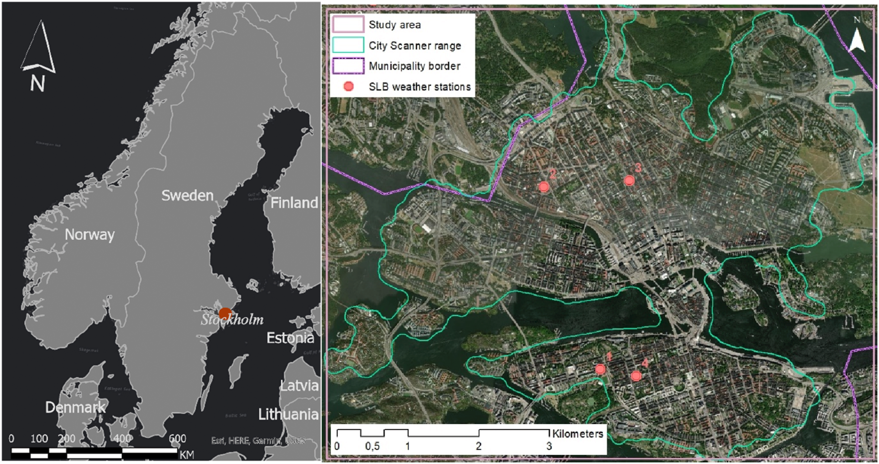

Once the DS platform detects movement through an accelerometer, it begins automatically taking measurements of a set of parameters: device ID; Tair (ambient); Tamb (ambient surface temperature for control); Tsurf (objects along the street); GPS coordinates in WGS-84; and date and time. Illustrations of the DS platform is available in Supplementary Materials, SM1. The data collection period was from the 26th of July to the 31st of August, 2021. The DS platform utilizes an opportunistic sensing approach, allowing the taxis to operate along their normal routes while collecting environmental data during the journey. Overall, ∼520k data points were captured from the deployment, distributed over 5 devices with a 5-s temporal resolution.

First, we analysed all hours that the DS platforms were active, with a speed >7 m/s (n = 108,184), and secondly, we focused on a subset of night-and-morning data from 0 to 10 am (n = 19,099), before the temperature reaches its peak. The purpose of separately analysing the night-and morning hours was to study the night-time temperatures, with high relevance for human health, while still capturing enough data for temporal and spatial coverage. Missing data was deleted case-wise.

Data treatment and analyses

To investigate how the DS data performed compared to other heat data sources, we used the four stationary weather stations (WSs) available within the study area (Figure 1), providing data on air temperature every 15 minutes (SLB-analys, 2021). We also used available RS data on Tlst derived from Landsat 8 with 100 × 100 m resolution, for comparison (USGS, 2022).

Other data used for the analyses included Google Street View (GSV) images (© Google) for calculating greenview and skyview indices, a digital elevation model of 2 × 2 m (Lantmäteriet, 2018), data on buildings (City of Stockholm, 2019), and road data (STA, 2021) for creating buffer zones, viewsheds, and sample spots. The spatial analyses were performed using ArcGIS Pro 2.9.0 (ESRI Inc., 2020), ArcMap 10.8.1 (ESRI Inc., 2011), and QGIS Desktop 3.22.1 (QGIS, 2022). For raster data, 2 × 2 m resolution was used for all analyses. For the statistical analyses, we used MATLAB R2022a (MathWorks Inc., 2022) and Statistica 13.4 (StatSoft, 2018).

Since the vehicles carrying the DS platforms moved in different directions on the streets, and the measuring device pointed perpendicular to the right, we separated the roads into two sides, applying buffer zones along the middle of the roads (STA, 2021). These buffer zones were 30 m wide to match the uncertainties of the GPS-derived coordinates. The heat data were then interpolated inside these buffer zones using diffusion within barriers, with 90 m maximum distance, in ArcGIS. Furthermore, inside the buffer zones, we created circular sample spots of 30 m diameter as a unit of assessment (Figure SM2).

First, the DS platform’s heat data was compared to Tair measurements taken by the four stationary WS (SLB-analys, 2021) (see Figure 1). This data is measured with a time step of 15 minutes, while the DS platforms have a time step of 5 seconds for each device and are not synchronized. To enable comparison, the data was aggregated using the average temperature over 1 hour for both datasets. The hourly deviation data was interpolated inside the buffer zones and sampled. Secondly, the DS platform’s heat data (Tsurf) was compared to the land surface temperature (Tlst) derived from a satellite image of Landsat 8 (USGS, 2022). It passed Stockholm on 8 August 2024 around 11 am. A sample of observations from the DS platform, matching the spatio-temporal window without clouds from the satellite image, was collected for comparison.

To estimate the sun exposure on the surfaces that the DS platforms measured, the digital elevation model on terrain (Lantmäteriet, 2018) was combined with building height data (City of Stockholm, 2019) to find the urban canyons in a combined urban elevation model of 2 × 2 m. For each hour the sun was up during the summer months, the shadow distribution was calculated using UMEP (Lindberg et al., 2018). In this way, the average sun exposure for each pixel could be estimated (Figure SM2).

Next, since the DS platforms only register data at the street-level, the rooftop surfaces of the building polygons were removed from the data. Finally, to avoid areas behind buildings and other obstacles that were not visible for the DS platforms, we calculated the visible areas from the middle of the roads using viewshed in ArcGIS. In this way, invisible areas could also be removed. The sun exposure for surfaces visible by the DS platforms was then used in a sun-exposure heat (SEH) index (equation (1)):

S E H = \frac{s u r f a c e t e m p e r a t u r e}{\log (s u n e x p o s u r e h o u r s)}

(1)

The SEH index was derived using samples of interpolated Tsurf and mean values of sun exposure hours per visible areas within the sample spots. It was used as a dependent variable, representing heat taking account of sun exposure. Furthermore, the density of the DS platform measurements varied across the sample spots of the study area, since the taxis visited different areas with different frequencies. Therefore, we tested to use only the sample spots with at least 128 measurements during the 36 monitored days, for which test N = 1556.

The influence of two predictive variables on the DS Tsurf data was analysed on the hyper-local scale. These were the percentage of visible greenery (greenview) and visible sky (skyview), both derived from GSV images from 2009 to 2012, 2014, and 2016–2021, using a computer vision algorithm. For this, we utilized the ADE20K dataset-based semantic segmentation model developed by Zhou et al. (2019) to perform pixel-level classification of common objects in street view images. By applying this model to our GSV images, we were able to calculate the proportion of sky and greenery pixels relative to the total number of pixels in each image. Greenview provides a measure of the greenery in immediate adjacency, while skyview provides additional insights into the urban canyons and building density along the roads (see e.g. Gong et al., 2018; Li and Ratti, 2018; Zhang et al., 2018). This point data was interpolated within the buffer zones and then sampled. The DS Tsurf, the SEH index, and their spatial distribution were then explained by green and grey structures in the urban landscape, using statistical methods in the form of Pearson correlation with a confidence interval of 95% and multiple linear regression (Krzywinski and Altman, 2015).

Results

The temperature data from the DS platforms along with the WS data are shown in Figure 2. Figure 2(a) shows hourly mean values of both the DS platforms and the WS data, between July 28th and August 6th 2021. The DS platforms measured temperatures very sparsely during the night, while the WSs measure continuously every 15 minutes. Overall, all the data follow a similar pattern, while the hourly mean of the datasets smooth out minor variations.

Figure 2.

Outcomes of the heat measurements from the DS platforms and comparisons with the stationary WSs. In (a) a snapshot between 28th of July and 6th of August 2021, hourly mean values of the measurements for both data sources. The DS platforms measure Tsurf and Tamb (measured with IR-device), and Tair, while the four WSs measure Tair. In (b) a scatterplot between the DS heat measurements and the corresponding hourly means of the WS data, for the whole monitored period. Maps of average temperatures across the 38 monitored days, interpolated within the road buffer zones, (c) DS Tsurf during night and morning hours, and (d) DS Tsurf for all hours during the day.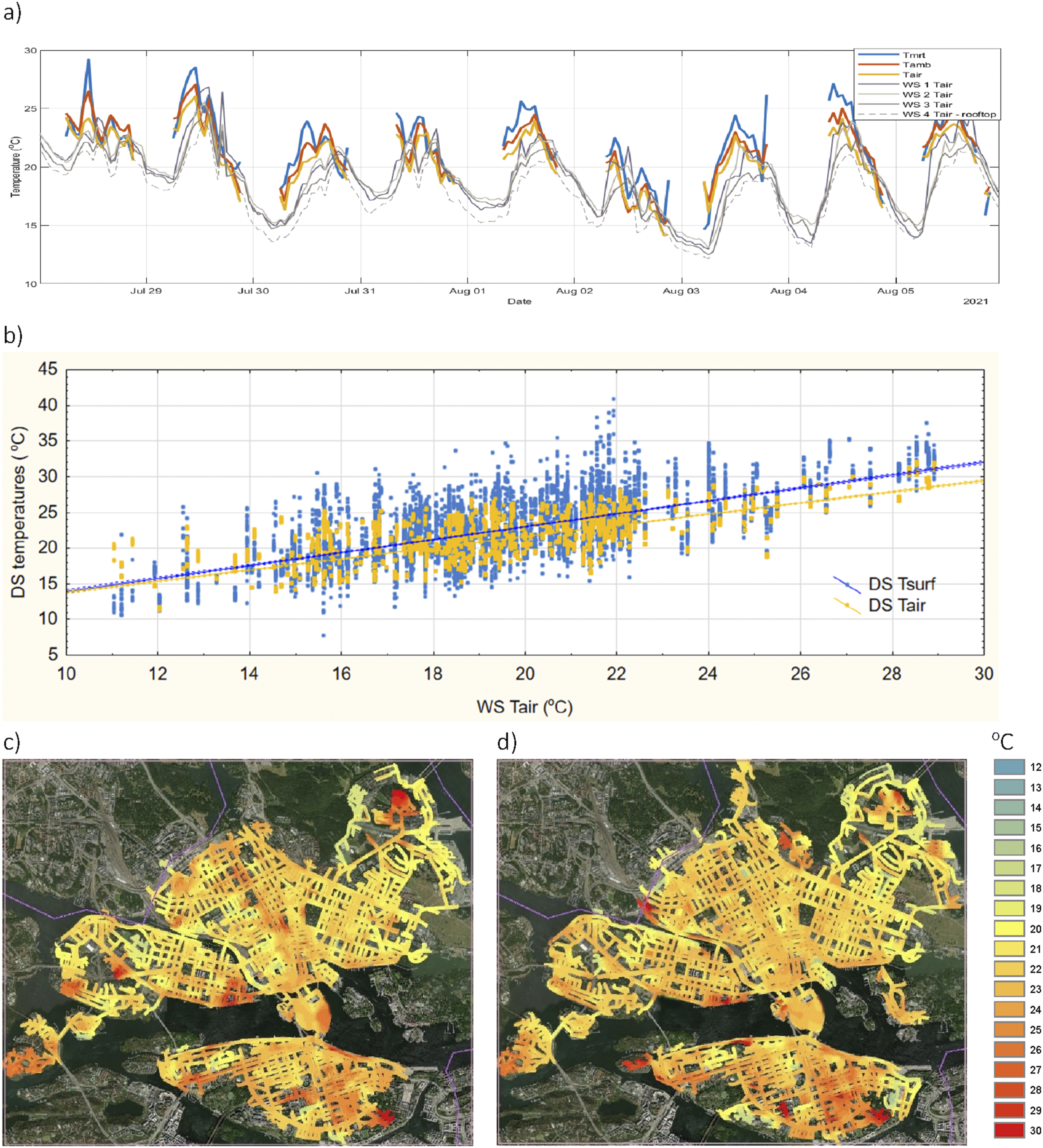

An internal comparison between the different DS heat data is illustrated in Figure SM3. The Tamb measured by the IR sensor was a control point of the IR device performance. The Tamb was strongly correlated to the Tair (R = 0.989, R² = 0.979, and p < .001), which indicates a good performance of the IR sensor. Tsurf also showed a high and significant correlation with the Tair measurements but with a much higher variation and more extreme values (Figure SM3). The average difference between DS Tsurf and DS Tair was 1.00°C, ranging from −15.2 to 22.8 (SD ± 2.5), the ratio Tair/Tsurf was 0.95, the correlation coefficient was 0.876, R² = 0.767, and p < .001.

The spatial pattern of Tsurf is illustrated in Figure 2(c) for morning hours and Figure 2(d) for all hours during the daytime. As can be seen, the data capture of the morning hours does not have the full spatial coverage of the all-day hours. Comparing these maps to each other, the all-day hours show overall higher temperatures and a more evenly spread heat pattern. In the morning hours, on a detailed scale, there are distinct hot zones and cool zones visible with higher and lower temperatures, respectively. In the all-day hours heat pattern, many of these zones seem to even out. Since these patterns represent all 36 investigated summer days in 2021, they provide interesting leads to the local urban climate.

Air temperature (Tair)

To enable further comparison between the measures of the DS platforms and the WSs, the WS data was aggregated into hourly averages for all the four stations and assigned to the corresponding hour of the DS platform measurements (Figure 2(b)) to account for the difference in sampling time intervals. Overall, the DS Tair aligned well with the WS Tair, with a correlation coefficient of = 0.796, R² = 0.633, and p < .001. However, the DS Tair measurements were generally higher than the WS Tair, with a mean difference of 1.21°C, ranging from −6.58 to 11.0°C (SD ± 1.87°C). Taking only morning hours into account, the mean difference was 2.97°C, with a range from −0.87 to 11.0°C (SD ± 1.43°C).

Surface temperature (Tsurf)

As expected, the DS Tsurf showed more extreme values than WS Tair and was on average higher. The DS Tsurf had a weaker but still statistically significant relation with the WS Tair (R = 0.643, R² = 0.414, and p < .001) (Figure 2(b)). The DS Tsurf data were generally higher with a mean difference to WS Tair of 2.20°C, ranging between −11.3 and 27.1°C (SD ± 3.02°C). For morning hours, the mean difference was 3.96°C, with a range between −6.7 and 24.7°C (SD ± 2.71°C).

Comparisons with other data sources

Figures 3(a) and 3(b) show differences for the sample spots between DS Tsurf and WS Tair, plotted against the DS Tsurf raw data. As shown in Figure 3(a), in the mornings, the DS Tsurf was consequently higher than WS Tair in almost all sample spots, while only 1.1 % of the sample spots had lower values. This changed somewhat when taking all-day hours into account (Figure 3(b)), but still, most of the sample spots had higher DS Tsurf than WS Tair, even if a certain amount (8.4 %) instead was lower. Overall, in the mornings, the heat differences were higher than taking all-day hours into account. In both cases, it is also obvious that the higher the DS Tsurf, the greater the difference to the WS Tair.

Figure 3.

Scatterplot (a) shows the relation between DS Tsurf heat (x-axis) compared to the difference between this and the WS Tair (y-axis), for night and morning hours (0–10 am) for the sample spots during the summer 2021, with (c) showing a corresponding map. Scatterplot (b) shows the same relation for all hours that the city scanner was active, with (d) showing the corresponding map.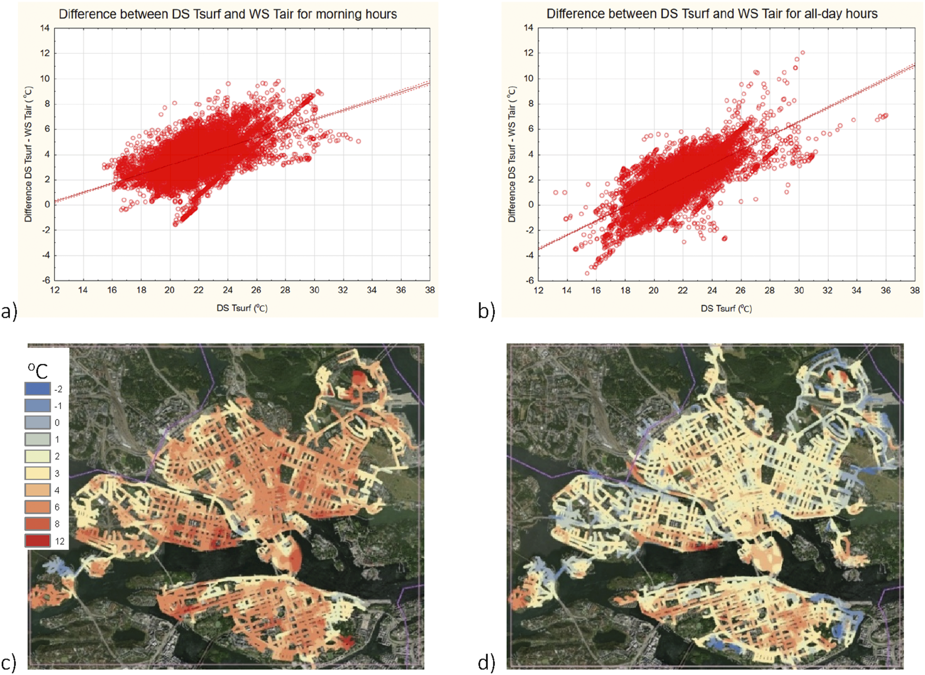

The spatial pattern of these differences, shown in Figures 3(c) and (d), reveals that in the mornings, the surfaces Tsurf were overall distinctly warmer than the corresponding WS Tair, suggesting that the urban objects stored heat overnight. When looking at all-day hours, the pattern evens out, and many surfaces are instead similar to WS Tair. In these maps, hot and cool zones are visible, with either higher or lower ΔT than their immediate surroundings.

In the next comparison, we related the DS Tsurf to RS Tlst, where the latter was derived from satellite images (Landsat 8). For this comparison, we selected a sample of Tsurf measurements from the DS platform that matched the time of the passing satellite as well spatially matched the cloud-free zone of that image. This yielded 186 measurement points with a central location in the study area. For each of these points, the DS Tsurf measurement was compared with RS Tlst for the same localization and time (11 pm ± 1 hour). Thus, the DS Tsurf measurements showed to have in average 3.3°C higher temperatures. DS Tsurf showed a mean temperature of 25.0°C, ranging between 19.8°C and 36.4°C, SD ± 3.32°C. Simultaneously, RS Tlst had a mean temperature of 21.7°C, ranging between 16.9 and 23.9°C, SD ± 1.71°C. The data comparison is plotted in Figure 4. Within this sample, the correlation between DS Tsurf and RS Tlst was weak but significant (R = 0.244, R² = 0.060, p < .001, N = 186). Without the outliers (marked in the Figure 4), it was stronger (R = 0.359, R² = 0.129, p < .0001, N = 178), but as can be seen, still with a high variation. A visual inspection of the outliers revealed that they all were pointing at facades mainly facing south and slightly east, which would be where the sun would heat the building surfaces at that time of the day.

Figure 4.

Comparison between Tlst and Tsurf, using the cloud-free zone of the central study area that was available during the 36 monitored days, that is, 9 august 2021 (n = 186). The encircled outlying values (a) were selected for visual inspection.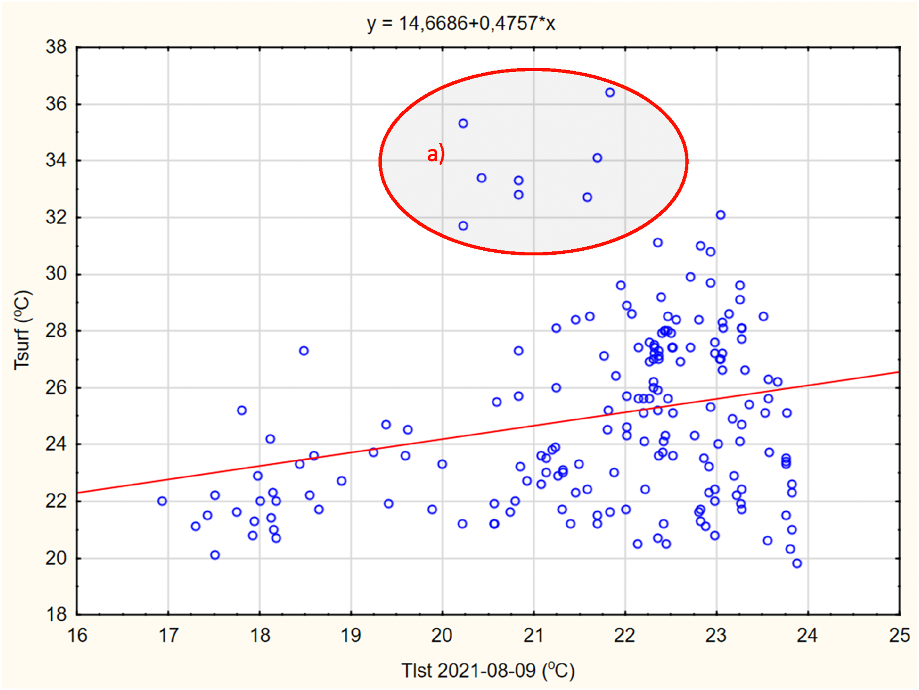

Influence of greenery and grey structures on urban heat

To investigate heat patterns as measured by the DS platforms, we used two predictive variables. Densely built-up areas have a warming effect and can be measured indirectly using the skyview factor. Furthermore, greenery generally has a cooling effect and can be measured through the greenview factor. The relations between DS Tsurf and the predictive variables skyview and greenview are illustrated in Figure 5. In addition, the SEH index was used as an alternative dependent variable to also take sun exposure into account.

As Figure 5 shows, a higher amount of visible sky is related to cooler temperatures, both represented by DS Tsurf (R = −0.174, R² = 0.030, and p < .001) and the SEH index (R = −0.476, R² = 0.226, and p < .001). Visible greenery also has a significant cooling effect, measured both via DS Tsurf (R = −0.150, R² = 0.022, and p < .001) or the SEH index (R = −0.434, R² = 0.189, and p < .001). These predictive variables partially overlap and combined in a multiple regression model allow us to explain DS Tsurf, Multiple R = 0.225 and R² = 0.050, and p < .001; while for the SEH index, Multiple R = 0.631, R² = 0.398, and p < .001. Thus, the SEH index, considering sun exposure, performed well to provide insights into how the Tsurf relates to greenery and grey structures in the urban landscape (Figure 5(c)).

As the density of DS platform measurements was uneven due to the opportunistic approach, we added a test using only the sample spots with at least 128 measurements during the 36 monitored days. In this test (N = 1556), the relations with skyview and greenview were even stronger; for skyview and DS Tsurf (R = −0.212, R² = 0.045, p < .001), skyview and the SEH index (R = −0.543, R² = 0.294, p < .001), as well as greenview and DS Tsurf (−0.400, R² = 0.160, p < .001) and greenview and the SEH index (R = −0.583, R² = 0.340, p < .001). When combined in a multiple regression model, DS Tsurf was predicted by these two variables (Multiple R = 0.394, R² = 0.155, p < .001) and so was the SEH index (Multiple R = 0.703, R² = 0.494, p < .001). Details of the equations for the SEH index are found in Table 1.

Table 1.

Details of the models using greenview and skyview for explaining the SEH index.

Sample 1 (spots with >8 samples)
N = 13967	Dependent variable: SEH-index
	R = 0.63079927, R² = 0.39790771, adjusted R² = 0.39782148
	F (2.13964) = 4614.2, p < 0.000, Std. error of estimate: 0.47525
	b*	Std. err	b	Std. err	t (13964)	p-Value
Intercept			4.86024	0.008332	583.3447	0.00000
Skyview_average	−0.457804	0.006573	−3.01693	0.043314	−69.6531	0.00000
Greenview_average	−0.414478	0.006573	−1.79407	0.028450	−63.0613	0.00000

Sample 2 (spots with >128 samples)
N = 2314	Dependent variable: SEH-index
	R = 0.70318397, R² = 0.49446770, adjusted R² = 0.49403020
	F (2.2311) = 1130.2, p < 0.000, Std. error of estimate: 0.37272
	b*	Std. err	b	Std. err	t (2311)	p-Value
Intercept			4.92747	0.016263	302.9776	0.00000
Skyview_average	−0.501083	0.014925	−3.25053	0.096819	−33.5732	0.00000
Greenview_average	−0.430688	0.014925	−2.17765	0.075464	−28.8567	0.00000

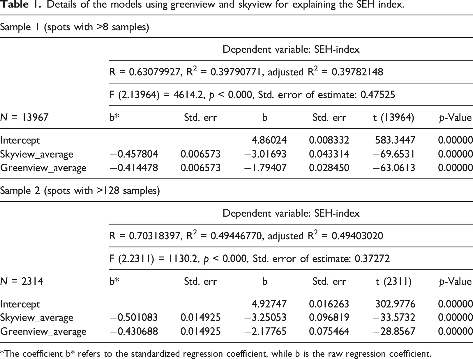
*The coefficient b* refers to the standardized regression coefficient, while b is the raw regression coefficient.

Discussion

Comparisons of temperature data sources

The DS platforms provided data on Tsurf and Tair with high spatial and temporal resolution, covering the urban landscape, which can be seen as promising for further analyses of UHI effects. In different ways, this data deviated from each other and from heat data of other sources with different spatial and temporal resolutions. The DS Tamb showed a strong correlation with the DS Tair measurements (Figure SM3), which indicates an overall good performance of the IR sensors. Comparing the DS platform measurements on Tsurf and Tair, Tsurf was generally higher, while the ratio between these was within the range of the ratios mentioned by Gunawardena et al. (2017). The correlation between them was high but with high variation and extreme values, as illustrated by Figure SM3.

There was a high correlation between the DS platform measurements of Tair and the stationary WS Tair. However, there was a deviation so that the DS Tair was generally higher; the mean difference was 1.21°C ranging from both cooler and hotter than WS Tair. When we only looked at morning hours, the mean difference was 2.97°C and mainly hotter than WS Tair. The deviation may have several reasons, and one could be related to the differences in height. The DS platforms mounted on the taxi vehicles were approximately 1.5 m above the paved roads, while the weather stations are situated 2 m above the ground, and in one case, situated on a rooftop. Differences in measured temperature between the data sources could also be due to the wider spatial coverage of the DS platforms, with a variety of urban landscape components, such as both denser and more sparsely built-up areas, greenery, waterfront, and other. By contrast, the stationary WSs are situated within a few kilometres of each other, in densely built-up urban areas with little vegetation.

Ziter et al. (2019) also used DS devices on a detailed scale in an urban landscape but instead mounted on bicycles. In their study, the Tair during daytime (13–19) was on average 0.59°C higher than the WS Tair reference data (SD ± 0.83°C). This study also covered different urban landscape components, like the current study; however, our DS Tair measurements covered also morning and evening hours so therefore the variation could be expected to be higher.

When we instead compare the DS platform data on Tsurf with the stationary WS Tair, the DS Tsurf was higher with a mean difference of 2.20°C, while for only morning hours, the mean difference was 3.96°C. To some extent, the differences could have similar reasons as for DS Tair, such as differences in height and spatial coverage. In addition to that, the Tsurf is related to the way heat is reflected, stored, and emitted for different surfaces, and direct exposure to sunlight will add to its variability. In particular, hard surfaces will accumulate heat during the day and may stay warm during nighttime. In Figure 2, the maps show that most of the study area was overall cooler in the morning hours compared to the all-day hours. Figure 3, however, instead shows the differences between Tsurf and WS Tair. As can be seen in both the scatter plots and the maps, ΔT was particularly high in the morning hours, which would be an indication of the urban heat storage at night.

Thus, the DS platform measurements revealed spatiotemporal patterns of urban heat, with higher ΔT between DS Tsurf and WS Tair in the morning hours than during all-day hours (Figure 3). Furthermore, the hot and cool zones were more distinct in the mornings and seemed to even out when looking at all-day hours (Figure 2). These spatiotemporal patterns of urban heat seem to mirror those found in other research, but instead for Tair in urban-rural comparisons. For instance, Oukawa et al. (2022) reported that the difference in Tair between urban and rural areas was higher during the night and early mornings but mild during the day. According to Sheng et al., 2017, the atmosphere is gradually heated by land surface radiation during the daytime, with the result that the spatial variations of Tair become smaller and smaller. At night, the land surface will radiate most of the energy absorbed and more energy will be released into the atmosphere in urban areas than in rural areas.

When relating the DS Tsurf data to RS Tlst, we used the spatio-temporal, cloud-free window when Landsat 8 passed over our study area. The correlation between these two measurements was clear, even with a low sample size of observations (n = 186), where Tsurf was in average 3.3°C higher and had a higher variability (Figure 4). It should be noted that the RS Tlst data was derived from Landsat 8, which passes Stockholm around 11 o’clock, when the temperature is not at its peak. Still, all the outliers marked in Figure 4 were pointing to sun-exposed facades, which should explain much of the variability. Several studies compare RS Tlst and WS Tair, where RS-derived measurements of Tlst have been found to show positive biases relative to WS Tair (Sheng et al., 2017; Venter et al., 2021). Likewise, Tan et al. (2017) found an overall difference between RS Tlst and WS Tair of about 1°C on a clear day. This is not directly comparable to our study but illustrates how data from different sources may deviate from each other.

The DS Tsurf data and the comparison (ΔT) between the DS Tsurf and WS Tair have some spatial similarities, visible when comparing the maps in Figures 2 and 3. For instance, in some places, the hot zones coincide spatially, especially along the waterfront. So, the presumed cooling effect of water bodies evident in studies based on RS Tlst (Lin et al., 2020; Wiman and Lindeberg, 2022) was not so evident in our DS Tsurf study.

In this context, it is noticeable that a study comparing RS Tlst and WS Tair (Tan et al., 2017) found that water had a higher RS Tlst error (regarding WS Tair as the reference) than the other land-cover types, of about 1.2°C, while the RS Tlst errors for buildings and vegetation were less than 0.75°C. Furthermore, in a meta-analysis, Gunawardena et al. (2017) identified cooling effects of waterbodies in urban areas primarily during the daytime. However, at night and particularly towards the end of the summer, under anticyclonic conditions, their study showed that a warming effect was more probable, possibly owing to the thermal inertia of water. This is also in line with Ampatzidis and Kershaw (2020), who found that RS studies tend to overestimate the cooling potential of blue space, which may provide warming at night under certain conditions. The heterogeneity of water-cooling effects in UHI contexts was confirmed by Kirschner et al. (2024) and Wang and Ouyang (2021). Therefore, water bodies need further investigation to provide useful information for urban planning for avoiding UHI.

Hot and cool zones related to greenery and grey structures

The DS Tsurf data as well as the ΔT between the DS Tsurf and WS Tair show local hot-zones and cool-zones, visible in Figures 2 and 3. On a detailed urban scale, it has been shown that there can be ΔT between localized hot and cool zones as large as ΔT between urban and rural areas (Buyantuyev and Wu, 2010; Jenerette et al., 2016; Ziter et al., 2019). For instance, in a study of DS Tair on a detailed scale, Ziter et al. (2019) detected differences between the hottest and coolest zones of up to 3.5°C, whereas WS Tair varied by only an average of 0.2°C during the same period. This is a consequence of the complicated urban landscape patterns, where, for example, tree canopy can co-exist with impervious surfaces, and grey and green features are integrated at fine scales (Zhou et al., 2017).

The effects of grey structures and greenery were studied through the skyview and greenview indices, describing the amount of visible sky and visible greenery at the street level. These variables had a cooling effect and overlap to a certain extent, so in combination using multiple linear regression, they formed a model to predict urban heat, especially for the SEH-index, taking sun exposure into account (Figure 5). For the SEH-index, the model explained 39.8 % of the variation for all sample spots, and 49.4% of the variation if only sample spots of high sampling density (i.e. > 128 observations) were taken into account.

Figure 5.

Comparison between DS Tsurf and the SEH index for all sample spots, vs (a) greenview influence on DS Tsurf and the SEH index, (b) skyview influence on DS Tsurf and the SEH index, and (c) greenview influence on DS Tsurf in combination with illustrating sample spots with high skyview factor in blue.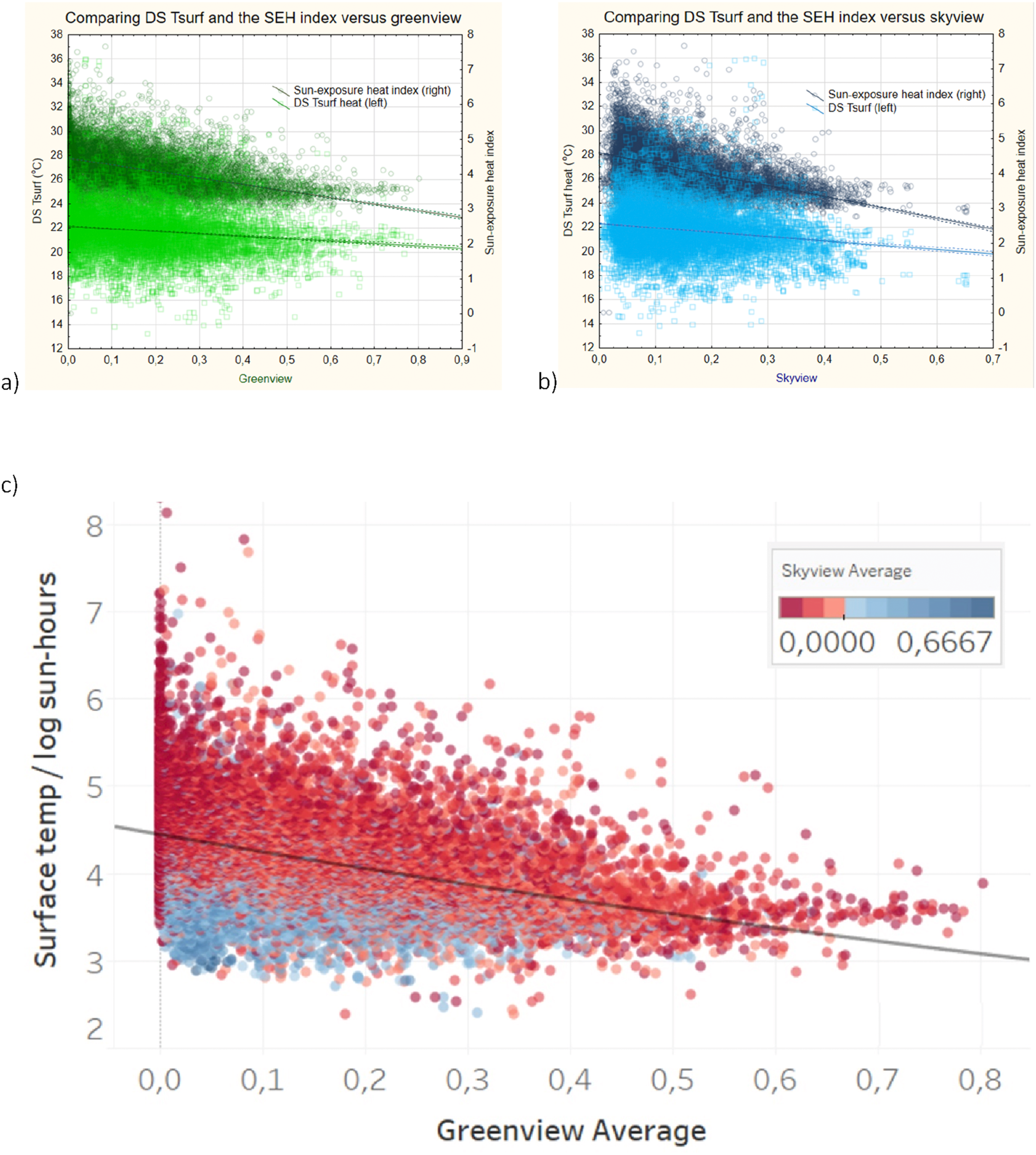

Thus, instead of only using the direct measurements of Tsurf, the SEH-index was developed to take into account the time that the different surfaces had been exposed to direct sunlight during the investigated summer days. The importance of sun exposure and shadows in studying and modelling Tsurf was addressed by several studies (e.g. Aleksandrowicz and Pearlmutter, 2023; Dorman et al., 2019; Lindberg and Grimmond, 2011; Zhao et al., 2020). For modelling shadows, we used raster-based modelling, using a high-resolution digital elevation model and detailed information on building heights (City of Stockholm, 2019). Another possibility would be to use more advanced shadow calculations based on vector data (Dorman et al., 2019). It is also possible to calculate shadows cast by trees and bushes (e.g. Lindberg and Grimmond, 2011), but in the current study, we chose to avoid that, to be able to separate the effect of local greenery on Tsurf.

Several studies on urban heat found a cooling effect of greenery (e.g. Greene and Millward, 2017; Gunawardena et al., 2017; Li et al., 2021; Ziter et al., 2019). Likewise, studies in Oslo (Venter et al., 2020) and New York City (Hamstead et al., 2016) found clear differences between grey and green surfaces also for cities in more northern latitudes, like Stockholm. In the current study, we related urban heat to skyview and greenview using multiple linear regression as a first test of the potential of our data. Further development paths will include using, for example, non-linear and machine learning models (Oukawa et al., 2022; Ziter et al., 2019). This will allow more in-depth analyses of the influence of multiple predicting variables, as well as taking spatial and temporal autocorrelation into account.

The DS approach for analysing UHI related to greenery

In studies on urban heat islands, stationary WSs are excellent for characterizing broad patterns and temporal dynamics but usually lack a more detailed spatial coverage (but see Schatz and Kucharik, 2014; Smoliak et al., 2015). RS data is very useful for studying urban heat patterns on larger spatial scales (Kim and Brown, 2021; Mirzaei, 2015), but due to the limited spatial and temporal resolution, it may miss hot and cool zones on a detailed scale, as well as short-time hot and cool periods. DS methods are increasingly used for environmental studies, as they can offer significant coverage with high resolution. The opportunistic DS approach in our study provided relatively good coverage of the centre parts of the City of Stockholm, but the spatial and temporal coverage was uneven due to lack of control over routes and travel schedules. Using only samples with a high sampling density, our model to explain Tsurf with the amount of visible sky and visible green improved. This further demonstrates the limitations of using opportunistic data and that the DS platform data needs additional calibration and data-cleaning procedures to ensure the data collected is accurate and useful (compare to e.g. Kumar et al., 2015; Xie et al., 2017).

In further research, we intend to expand the analyses to include a combination of the hyper-local scale with larger scales in the urban landscape (e.g. Gunawardena et al., 2017; Li and Schmidt, 2024) to further explore the urban grey and green patterns and their influence on urban heat, in a way that is useful for informing urban planning. For instance, greenery may influence urban heat on different scales. Ziter et al. (2019) used variable distances to represent the influence of greenery, while other studies found that greenery within 500 m was among the most relevant urban morphology parameters for explaining urban heat (Doick et al., 2014; Theeuwes et al., 2017). Further investigations of the influence of other land cover types on urban heat would also be interesting, such as differentiating between built-up and paved areas, as well as water bodies.

Another aspect that can be further investigated using our DS approach is the temporal dynamics of urban heat. The difference between Tlst and Tair has been shown to be maximized during daytime and minimized at night (Venter et al., 2021), while Bechtel et al. (2017) found a time lag of a few hours when comparing them. Furthermore, both Ziter et al. (2019) and Venter et al. (2021) found that Tair in daytime was best explained by greenery, while at nighttime, it was more related to hard surfaces. Therefore, the ground-measured Tsurf will be an important complement to Tair, since health impacts of urban heat are mainly related to nighttime heat (He et al., 2022). Thus, ground-measured Tsurf can be seen as a key factor in understanding the relationship between the local dynamics of out-door Tair and indoor temperatures which affect people most during the night.

The data collected by the DS platform in this study helped to identify urban hot and cool zones on hyperlocal scales. In comparison, the DS methods provide opportunities to measure urban heat at data-sparse hyper-local scales and along continuous urban landscape gradients. The DS Tsurf measurements come from the average of objects reached by the sensor, so it registers urban heat from street-level objects. This information about the urban microclimate can provide better insights into what inhabitants and visitors of different areas perceive. Furthermore, it is useful for informing ecosystem service models (e.g. Goldenberg et al., 2017; Venter et al., 2020) that can provide planning support. Thus, the effect of greenery on urban heat indicates a need to balance greenery and grey structures in planning for sustainable urban development. Here, only structures visible from the street were analysed, but further analyses of effects on hyper-local urban heat from greenery and grey structures on larger scales will be a next step. In this process, our DS approach provides low-cost monitoring of urban heat with a high level of detail across the urban landscape. This novel approach allows UHI analyses that can give insights that are useful to support urban planning.

Supplemental Material

Supplemental Material - Assessing the impact of greenery on urban heat using opportunistic drive-by sensing

Supplemental Material for Assessing the impact of greenery on urban heat using opportunistic drive-by sensing by Elina Merdymshaeva, Simone Mora, Yuki Machida, Fan Zhang, Fábio Duarte, Sanjana Paul, Carlo Ratti, and Ulla Mörtberg in Environment and Planning B: Urban Analytics and City Science.

Footnotes

Acknowledgments

The authors acknowledge the support from the reference group, with special thanks to Lukas Ljungqvist, City of Stockholm.

Author contributions

Elina Merdymshaeva: Conceptualization, methodology, validation, data curation, and writing – original draft; Simone Mora: Conceptualization, methodology, supervision, project administration, and writing – review and editing; Yuki Machida: Methodology, writing – review and editing; Fábio Duarte: Conceptualization, methodology, supervision, project administration, writing – review and editing, and funding acquisition; Fan Zhang: Resources and software; Sanjana Paul: Conceptualization and writing – original draft; Carlo Ratti: Supervision and funding acquisition; Ulla Mörtberg: Conceptualization, methodology, validation, writing – original draft, project administration, supervision, and funding acquisition. All authors read and approved the final manuscript.

Declaration of conflicting interests

The author(s) declared no potential conflicts of interest with respect to the research, authorship, and/or publication of this article.

Funding

The author(s) disclosed receipt of the following financial support for the research, authorship, and/or publication of this article: This study was funded by Senseable Stockholm Lab () and the Swedish strategic research program StandUp for Energy. The funders played no role in study design, data collection, analysis and interpretation of data, or the writing of this manuscript.

ORCID iDs

Simone Mora

Fabio Duarte

Ulla Mortberg

Data availability statement

The dataset collected using the City Scanner DS platform during the current study is available in the Zenodo repository, https://doi.org/10.5281/zenodo.14531322 (Mora, 2024).

Supplemental Material

Supplemental material for this article is available online.

Elina Merdymshaeva is a PhD student at the Dept. of Sustainable Development, Environmental Science and Engineering, KTH Royal Institute of Technology, Stockholm, Sweden, within Land and Water Resources Engineering. Her research focuses on spatial analysis of urban heat and ecosystem services, geoinformatics and geostatistical modelling.

Simone Mora is a Research Scientist at the Massachusetts Institute of Technology (MIT) and an Adjunct Associate Professor at the Norwegian University of Science and Technology (NTNU). He does research on novel sensing technologies and their applications for future cities. He develops methods and tools for rapid design and rapid prototyping of internet-connected sensors and human-computer interfaces. He lectures in the field of design thinking, internet of things and environmental sensing. He has contributed to more than sixty scientific papers, he has been a visiting scholar at City London University, and he co-founded a company that developed an ideation toolkit to tackle the UN's Sustainable Development Goals.

Yuki Machida is the founder of Ambient Works and a former Research Fellow at MIT’s Senseable City Lab. His research focuses on the intersection of design, environment, health, and sensing technologies.

Fan Zhang is an Assistant Professor at the Institute of Remote Sensing and Geographical Information System, Peking University. He was a Senior Research Fellow at MIT and the leader of the Urban Visual AI group at the MIT Senseable City Lab. His research sits at the intersection of urban Informatics and geospatial artificial intelligence. He has published over 60 papers in journals including PNAS and Nature Communications.

Fabio Duarte is a principal research scientist at the Massachusetts Institute of Technology, and Associate Director of the Senseable City Lab. Duarte is the co-author of “Urban play: make-believe, technology, and space” (MIT Press).

Sanjana Paul is a graduate student in the Department of Urban Studies and Planning at the Massachusetts Institute of Technology, and a research assistant for the Science Impact Collaborative.

Carlo Ratti is a professor of the practice at the Massachusetts Institute of Technology, and Founder and Director of the Senseable City Lab. Ratti is the curator of the 2025 Venice Biennale of Architecture, and co-author of “Atlas of the Senseable City” (Yale University Press).

Ulla Mörtberg is a professor with research focus on spatial and environmental systems analysis at the Dept. of Sustainable Development, Environmental Science and Engineering, KTH Royal Institute of Technology, Stockholm, Sweden. Her research concerns analysis and assessment of sustainability of urban and landscape systems, including integration of ecosystem services and other sustainability aspects in planning and decision support.

References

Aleksandrowicz

Pearlmutter

(2023) The significance of shade provision in reducing street-level summer heat stress in a hot mediterranean climate. Landscape and Urban Planning 229: 104588.

Ampatzidis

Kershaw

(2020) A review of the impact of blue space on the urban microclimate. The Science of the Total Environment 730: 139068.

Bechtel

Zakšek

Oßenbrügge

, et al. (2017) Towards a satellite based monitoring of urban air temperatures. Sustainable Cities and Society 34: 22–31.

Burkhard

Kroll

Nedkov

, et al. (2012) Mapping ecosystem service supply, demand and budgets. Ecological Indicators 21: 17–29.

Buyantuyev

(2010) Urban heat islands and landscape heterogeneity: linking spatiotemporal variations in surface temperatures to land-cover and socioeconomic patterns. Landscape Ecology 25: 17–33.

Chapman

Bell

(2017) Can the crowdsourcing data paradigm take atmospheric science to a new level? A case study of the urban heat island of London quantified using netatmo weather stations. International Journal of Climatology 37: 3597–3605.

City of Stockholm (2019) Building polygons with heights. Stockholms stadsbyggnadskontor.

Clarke

(1972) Some effects of the urban structure on heat mortality. Environmental Research 5: 93–104.

Cummings

Stewart

Reist

, et al. (2021) Mobile monitoring of air pollution reveals spatial and temporal variation in an urban landscape. Frontiers in Built Environment 7: 648620.

10.

Depecker

Menezo

Virgone

, et al. (2001) Design of buildings shape and energetic consumption. Building and Environment 36: 627–635.

11.

deSouza

Anjomshoaa

Duarte

, et al. (2020) Air quality monitoring using mobile low-cost sensors mounted on trash-trucks: methods development and lessons learned. Sustainable Cities and Society 60: 102239.

12.

Doick

Peace

Hutchings

(2014) The role of one large greenspace in mitigating London’s nocturnal urban heat island. Science of the Total Environment 493: 662–671. doi: 10.1016/j.scitotenv.2014.06.048.

13.

Dorman

Erell

Vulkan

, et al. (2019) Shadow: R package for geometric shadow calculations in an urban environment. The R Journal 11: 287.

14.

ESA (2022) Sentinel-3. Paris: European Space Agency. https://sentinels.copernicus.eu/web/sentinel/missions/sentinel-3.

15.

ESRI Inc (2011) ArcMap 10.8.1. Redlands, California, USA: Environmental Systems Research Institute.

16.

ESRI Inc. (2020) ArcGIS Pro Version 2.5. Redlands, California, USA: Environmental Systems Research Institute.

17.

Goldenberg

Kalantari

Cvetkovic

, et al. (2017) Distinction, quantification and mapping of potential and realized supply-demand of flow-dependent ecosystem services. Science of the Total Environment 593-594: 599–609. doi: 10.1016/j.scitotenv.2017.03.130.

18.

Gong

F-Y

Zeng

Z-C

Zhang

, et al. (2018) Mapping sky, tree, and building view factors of street canyons in a high-density urban environment. Building and Environment 134: 155–167.

19.

Greene

Millward

(2017) Getting closure: the role of urban forest canopy density in moderating summer surface temperatures in a large city. Urban Ecosystems 20: 141–156.

20.

Gunawardena

Wells

Kershaw

(2017) Utilising green and bluespace to mitigate urban heat island intensity. The Science of the Total Environment 584: 1040–1055.

21.

Guo

Aviv

Loyola

, et al. (2020) On the understanding of the mean radiant temperature within both the indoor and outdoor environment, a critical review. Renewable and Sustainable Energy Reviews 117: 109207.

22.

Hamstead

Kremer

Larondelle

, et al. (2016) Classification of the heterogeneous structure of urban landscapes (STURLA) as an indicator of landscape function applied to surface temperature in New York City. Ecological Indicators 70: 574–585.

23.

Kim

Hashizume

, et al. (2022) The effects of night-time warming on mortality burden under future climate change scenarios: a modelling study. The Lancet Planetary Health 6: e648–e657.

24.

Jenerette

Harlan

Buyantuev

, et al. (2016) Micro-scale urban surface temperatures are related to land-cover features and residential heat related health impacts in Phoenix, AZ USA. Landscape Ecology 31: 745–760.

25.

Keeler

Hamel

McPhearson

, et al. (2019) Social-ecological and technological factors moderate the value of urban nature. Nature Sustainability 2: 29–38.

26.

Keesstra

Nunes

Novara

, et al. (2018) The superior effect of nature based solutions in land management for enhancing ecosystem services. The Science of the Total Environment 610-611: 997–1009.

27.

Kim

Brown

(2021) Urban heat island (UHI) variations within a city boundary: a systematic literature review. Renewable and Sustainable Energy Reviews 148: 111256.

28.

Kirschner

Moravec

Macků

, et al. (2024) Comparing the effects of green and blue bodies and urban morphology on land surface temperatures close to rivers and large lakes. Land 13(2): 162. doi: 10.3390/land13020162.

29.

Krämer

Kabisch

(2022) Parks under stress: air temperature regulation of urban green spaces under conditions of drought and summer heat. Frontiers in Environmental Science 10: 849965.

30.

Krzywinski

Altman

(2015) Multiple linear regression. Nature Methods 12: 1103–1104.

31.

Kumar

Morawska

Martani

, et al. (2015) The rise of low-cost sensing for managing air pollution in cities. Environment International 75: 199–205.

32.

Lantmäteriet (2018) GSD Höjddata grid 2+ [elevation data]. Lantmäteriet, https://dike.slu.se/get/ (accessed 2020-05-20).

33.

Ratti

(2018) Mapping the spatial distribution of shade provision of street trees in Boston using google street view panoramas. Urban Forestry and Urban Greening 31: 109–119.

34.

Schmidt

(2024) Can spatial patterns mitigate the urban heat island effect? Evidence from German metropolitan regions. Environment and Planning B: Urban Analytics and City Science 51(8): 23998083241227500. doi: 10.1177/23998083241227500.

35.

Zhou

Glockmann

, et al. (2021) Context sensitivity of surface urban heat island at the local and regional scales. Sustainable Cities and Society 74: 103146.

36.

Lin

Wang

Jim

, et al. (2020) Water as an urban heat sink: blue infrastructure alleviates urban heat island effect in mega-city agglomeration. Journal of Cleaner Production 262: 121411.

37.

Lindberg

Grimmond

(2011) The influence of vegetation and building morphology on shadow patterns and mean radiant temperatures in urban areas: model development and evaluation. Theoretical and Applied Climatology 105: 311–323.

38.

Lindberg

Grimmond

Gabey

(2018) Urban multi-scale environmental predictor (UMEP) - an integrated tool for city-based climate services. Environmental Modelling & Software 99: 70–87.

39.

Lüthi

Fairless

Fischer

, et al. (2023) Rapid increase in the risk of heat-related mortality. Nature Communications 14: 4894.

40.

Maes

Jacobs

(2017) Nature‐based solutions for Europe's sustainable development. Conservation letters 10: 121–124.

41.

MathWorks Inc. (2022) MATLAB and Statistics Toolbox Release 2022a. Natick, Massachusetts, USA: MathWorks Inc.

42.

Mirzaei

(2015) Recent challenges in modeling of urban heat island. Sustainable Cities and Society 19: 200–206.

43.

Mirzaei

Haghighat

(2010) Approaches to study urban heat island – abilities and limitations. Building and Environment 45: 2192–2201.

44.

Mora

(2024) Hyperlocal Urban Heat Data with a Mobile Platform [Data set]. Zenodo. https://doi.org/10.5281/zenodo.14531322.

45.

NASA (2022) MODIS: Moderate Resolution Imaging Spectroradiometer. National Aeronautics and Space Administration. Available at: https://modis.gsfc.nasa.gov/data/.

46.

Naughton

McDonald

(2019) Evaluating the variability of urban land surface temperatures using drone observations. Remote Sensing 11: 1722.

47.

Obradovich

Migliorini

Mednick

, et al. (2017) Nighttime temperature and human sleep loss in a changing climate. Science Advances 3: e1601555.

48.

Oke

Mills

Christen

, et al. (2017) Urban Climates. Cambridge, UK: Cambridge University Press.

49.

Oukawa

Krecl

Targino

(2022) Fine-scale modeling of the urban heat island: a comparison of multiple linear regression and random forest approaches. The Science of the Total Environment 815: 152836.

50.

Phelan

Kaloush

Miner

, et al. (2015) Urban heat island: mechanisms, implications, and possible remedies. Annual Review of Environment and Resources 40: 285–307.

51.

QGIS (2022) QGIS Desktop 3.22.1, QGIS Geographic Information System. London, UK: QGIS Association.

52.

Quaranta

Dorati

Pistocchi

(2021) Water, energy and climate benefits of urban greening throughout Europe under different climatic scenarios. Scientific Reports 11: 12163.

53.

Rodríguez

Melgar

Márquez

JMA

(2022) Assessment of aerial thermography as a method of in situ measurement of radiant heat transfer in urban public spaces. Sustainable Cities and Society 87: 104228.

54.

Roth

(2013) Urban heat islands. In: Fernando

(ed) Handbook of Environmental Fluid Dynamics: Systems, Pollution, Modeling, and Measurements. Boca Raton: Taylor and Fancis, Vol. 2, 143–162.

55.

Santamouris

(2018) Minimizing Energy Consumption, Energy Poverty and Global and Local Climate Change in the Built Environment: Innovating to Zero: Causalities and Impacts in a Zero Concept World. Amsterdam, The Netherlands: Elsevier.

56.

Santamouris

Ding

Osmond

(2019) Urban heat island mitigation. In: Newton

Prasad

Sproul

, et al. (eds) Decarbonising the Built Environment: Charting the Transition. Singapore: Springer Singapore, 337–355.

57.

Schatz

Kucharik

(2014) Seasonality of the urban heat island effect in Madison, Wisconsin. Journal of Applied Meteorology and Climatology 53: 2371–2386.

58.

Schwarz

Schlink

Franck

, et al. (2012) Relationship of land surface and air temperatures and its implications for quantifying urban heat island indicators—an application for the city of Leipzig (Germany). Ecological Indicators 18: 693–704.

59.

Sheng

Tang

You

, et al. (2017) Comparison of the urban heat island intensity quantified by using air temperature and landsat land surface temperature in Hangzhou, China. Ecological Indicators 72: 738–746.

60.

SLB-analys (2021) Weather and air quality data. East Sweden air quality and noise management association. City of Stockholm.

61.

Smoliak

Snyder

Twine

, et al. (2015) Dense network observations of the twin cities canopy-layer urban heat island. Journal of Applied Meteorology and Climatology 54: 1899–1917.

62.

Song

Park

(2020) Verification of accuracy of unmanned aerial vehicle (UAV) land surface temperature images using in-situ data. Remote Sensing.

63.

STA (2021) National Road Database. Borlänge: Swedish Transport Agency. Available at: https://www.nvdb.se/sv.

64.

StatSoft (2018) Statistica 13. Tulsa, OK: StatSoft.

65.

Tan

Liao

, et al. (2017) Land surface temperature retrieval from landsat 8 data and validation with geosensor network. Frontiers of Earth Science 11: 20–34.

66.

Theeuwes

Steeneveld

Ronda

, et al. (2017) A diagnostic equation for the daily maximum urban heat island effect for cities in northwestern Europe. International Journal of Climatology 37: 443–454.

67.

Tuholske

Caylor

Funk

, et al. (2021) Global urban population exposure to extreme heat. Proceedings of the National Academy of Sciences of the United States of America 118.

68.

USGS (2022) Landsat 8. United States geological survey. https://www.usgs.gov/landsat-missions/landsat-8.

69.

USGS (2023) Landsat 8. United States geological survey. https://www.usgs.gov/landsat-missions/landsat-8.

70.

Van Someren

EJW

(2003) Thermosensitivity of the circadian timing system. Sleep and Biological Rhythms 1: 55.

71.

Venter

Krog

Barton

(2020) Linking green infrastructure to urban heat and human health risk mitigation in Oslo, Norway. The Science of the Total Environment 709: 136193.

72.

Venter

Chakraborty

Lee

(2021) Crowdsourced air temperatures contrast satellite measures of the urban heat island and its mechanisms. Science Advances 7: eabb9569.

73.

Wang

Ouyang

(2021) Investigating the heterogeneity of water cooling effect for cooler cities. Sustainable Cities and Society 75: 103281.

74.

Wiman

Lindeberg

(2022) Temperaturanalyser från satellit. Stockholm: City of Stockholm, 42.

75.

Wong

Tan

Kolokotsa

, et al. (2021) Greenery as a mitigation and adaptation strategy to urban heat. Nature Reviews Earth & Environment 2: 166–181.

76.

Xie

Semanjski

Gautama

, et al. (2017) A review of urban air pollution monitoring and exposure assessment methods. ISPRS International Journal of Geo-Information 6: 389.

77.

Yang

(2015) The impact of building density and building height heterogeneity on average urban albedo and street surface temperature. Building and Environment 90: 146–156.

78.

Zhang

Liu

, et al. (2018) Representing place locales using scene elements. Computers, Environment and Urban Systems 71: 153–164.

79.

Zhao

Luo

(2020) Analysis of the thermal environment in pedestrian space using 3D thermal imaging. Energies 13: 3674.

80.

Zhao

Wang

, et al. (2021) Urban air pollution mapping using fleet vehicles as mobile monitors and machine learning. Environmental Science and Technology 55: 5579–5588.

81.

Zhou

Pickett

STA

Cadenasso

(2017) Shifting concepts of urban spatial heterogeneity and their implications for sustainability. Landscape Ecology 32: 15–30.

82.

Zhou

Zhao

Puig

, et al. (2019) Semantic understanding of scenes through the ade20k dataset. International Journal of Computer Vision 127: 302–321.

83.

Ziter

Pedersen

Kucharik

, et al. (2019) Scale-dependent interactions between tree canopy cover and impervious surfaces reduce daytime urban heat during summer. Proceedings of the National Academy of Sciences 116: 7575–7580.

Supplementary Material

Please find the following supplemental material available below.

For Open Access articles published under a Creative Commons License, all supplemental material carries the same license as the article it is associated with.

For non-Open Access articles published, all supplemental material carries a non-exclusive license, and permission requests for re-use of supplemental material or any part of supplemental material shall be sent directly to the copyright owner as specified in the copyright notice associated with the article.

0.00 MB

0.85 MB