A high-resolution global time series of street-network sprawl

Abstract

Systems of street networks form a backbone for many aspects of human life and, once laid down, urban streets represent a nearly immutable influence on future urban form and concomitant travel, energy, and social outcomes. Moreover, as humanity is currently passing through its peak urbanization rate, decisions about how to design such networks at the local scale are being made faster than ever before. In this work, we quantify local street connectivity and provide a global, high-resolution time series of our Street Network Disconnectedness Index (SNDi) as an open data set. We derive a stylized version of the actual geographic road network from the 2023 vintage of OpenStreetMap by simplifying complex intersections, divided roads, and offset intersections. Using this functional representation of the network corrects systematic biases in derived properties of the network. We couple this simplified network with a newly available time series of urbanization in order to compute SNDi and provide a dynamic analysis to the year 2019 and a cross-sectional analysis for 2023. We release our data as the raw network of edges and nodes and as aggregates to a 1 km grid, to countries, and to five subnational administrative levels. We also provide interactive visualizations at sprawlmap.org. Overall, our findings present a picture of rapidly worsening street-network connectivity in many regions of the world.

Introduction

Street networks are a key dimension of urban form. The connectivity of streets shapes the travel choices and carbon footprints of a city’s residents (Barrington-Leigh and Millard-Ball, 2017; Ewing and Cervero, 2010), and possibly long-term densification opportunities as well. Less-connected streets—which we call street-network sprawl—reduce accessibility by bus, walking and cycling, partly because their greater circuity increases travel distances and makes public transportation service less feasible.

The importance of today’s decisions on street-network sprawl is amplified by lock-in and by the rate of change. Once laid down, street patterns rarely change, even after fires, wartime bombing, and earthquakes (Vazquez et al., 2023). And given that growth in the urban population is expected to peak by 2025 (United Nations, 2019), it is likely that the 2020s will also represent the period of peak growth in urban street construction.

Our previous work (Barrington-Leigh and Millard-Ball, 2019, 2020) reported aggregate estimates of street-network sprawl for all countries and 200 selected cities. In this paper, we offer three major advances. First, we release for the first time the full data at the 1 km level as a global grid, as well as the underlying street and path network as a graph of nodes and edges. In our earlier work and in this new dataset, we use raw data from OpenStreetMap (OSM) to compute 13 measures of connectivity, which we aggregate into a single index—the Street Network Disconnectedness Index (SNDi). Second, we offer a new algorithm for transforming the geometric representation of the street network into a simplified graph that is more appropriate for network analysis. Third, we update our cross-sectional data to use the October 2023 vintage (i.e., version) of OSM, and update the time series to examine shifts in street-network sprawl from 2015 to 2019, taking advantage of new longitudinal datasets on urban growth.

Our dataset complements the availability of global-scale population density (Florczyk et al., 2019; ORNL, 2011) and street connectivity datasets for specific countries (Boeing, 2020). Many analyses of urban form focus exclusively on population density, given the ready availability of data derived from national censuses and remotely sensed nighttime lights. Our street-network sprawl data provide a complement that reflects a separate and more enduring dimension of urban form. Our work is closest to that of Boeing (2021) who provides street connectivity indicators for each urban center in the world. We go beyond that to (i) provide a time series from 1975 to 2020; (ii) provide measures for a 1 km grid that is not confined to urban center boundaries; (iii) include bicycle and pedestrian paths that are omitted from the Boeing dataset but are crucial in the connectivity of streets in places such as Denmark (Barrington-Leigh and Millard-Ball, 2020); and (iv) simplify the street network to provide more meaningful measures of connectivity.

Our contributions in this paper are (i) producing a dataset for other researchers to use and build on, (ii) providing descriptive analysis of geographic patterns in street-network sprawl and trends over time, and (iii) identifying and addressing how to simplify a geometric road network for purposes of network and connectivity analysis. As we discuss below, simplification is important to avoid double counting complex intersections that are represented by multiple nodes, and roads with a median that are represented by multiple edges. As this is a “data” paper, we do not identify or test specific hypotheses or theoretical mechanisms, but our data can facilitate future research in the vein of regional and global-scale studies on the impact of street connectivity on urban history (Salazar, 2021; Vazquez et al., 2023), transportation choices (Brenner et al., 2024; Hajrasouliha and Yin, 2015; Marshall and Garrick, 2010), environmental outcomes (Rezaei and Millard-Ball, 2023), social relations, and more.

Measuring street-network sprawl

Street-network sprawl—our term for low street connectivity—is often quantified as the proportion of deadends or four-way intersections, average nodal degree, and/or intersection density (Ewing and Cervero, 2010; Marshall and Garrick, 2010). In North America, the empirical setting for most street connectivity research to date, these measures can distinguish between two of the most common street-network configurations—a grid (where most nodes are degree-4) and subdivisions with culs-de-sac (where most nodes are degree-3 or degree-1). But nodal degree does not do justice to the connectivity of irregular networks typical of many Japanese, Middle Eastern, and European cities, where most nodes are degree-3 but pedestrian connectivity is clearly high.

Therefore, we quantify street-network sprawl using a wider range of attributes that can distinguish between more- and less-connected streets in a range of different urban design traditions. In addition to nodal degree and the fraction of deadends, we use measures of circuity (the ratio between network distance and Euclidean distance) and sinuosity (the curviness of individual street edges). We also include several measures of the network function of each edge based on their graph theoretic properties. For example, we calculate the number and fraction of network “bridges”—streets that are the only connection between two different parts of the network, such as the single entrance to a gated community. Our 13 measures are described in Table A2 in the Appendix.

We collapse these 13 measures to a single index, the Street Network Disconnectedness index (SNDi) by using their first principal component (Table A3). Higher SNDi indicates more street-network sprawl, that is, less-connected streets. In our previous work, we validated SNDi using Google Street View imagery and national census data, and showed that SNDi corresponds to neighborhood walkability as well as individual decisions on car ownership and commute mode. The updated Principal Component Analysis (PCA) coefficients reported in Table A3 are similar to our previous estimates, indicating that our newly calculated SNDi has a similar interpretation.

Most of our analysis was carried out in a PostgreSQL/PostGIS database, with scripting and some network analysis functions undertaken in Python. We made use of moderate parallelization (56 processors) for many tasks, and of the ∼0.7 TB RAM available on our dedicated computation server. The entire planet took us about 1 month to process. The two most lengthy stages were the road network simplification ( ∼12 days) and the calculations of circuity and graph theoretic properties for each node ( ∼14 days).

In general, our computational approach is similar to that described in our 2019 analysis. In the following sections, we briefly describe that approach, and focus in more detail on the changes we have made. In the Appendix, we provide a more extensive step-by-step discussion of our algorithm and show the impact of the change to our algorithm and of updating the underlying OSM data from the 2019 to the 2023 vintage.

Simplifying the network

Maps that are geometrically accurate are not necessarily well-suited for network analysis and analyzing the connectivity of streets. Three examples are illustrative. In one case, a roundabout is functionally a single intersection, but geometrically, the roundabout may be depicted as a circular street, with each entrance (and possibly exit) accounting for a separate intersection. In another case, a slightly staggered intersection is functionally a degree-4 node but geometrically might be represented as two degree-3 nodes, connected by a very short street. In a third case, a two-way street might be represented as two different one-way streets due to the presence of a median. In all three cases, using the geometric rather than the functional representation will tend to bias upwards the number of nodes and also affect other properties of the network. Such biases will also inflate other measures often used in the urban planning literature, such as intersection density.

For this reason, we develop an algorithm to simplify the geometric representation of the street network provided by OSM. Our overall philosophy is to mitigate the dependence of our results on how the street network is represented in OSM—for example, the mapper may depict a staggered intersection with two nodes rather than a single node, map sidewalks as separate edges from the roadway, or represent a road with a median as two parallel edges, one for each direction. Note that this is conceptually separate from our process of annealing—that is, removing nodes that are degree-2 (not intersections or deadends). While this annealing is called “simplification” by Boeing (2017), our simplification process goes beyond this.

We also simplified the network in our 2019 analysis, but here we improve on that approach in two ways related to (i) complex intersections and (ii) divided roads. We summarize our algorithm here and provide more detail in the appendix.

Complex intersections

Complex intersections include roundabouts, staggered intersections, and motorway interchanges that are functionally a single intersection but are represented as multiple nodes in OpenStreetMap. In our 2019 analysis, we identified clusters where all nodes were within 20m of another node, and collapsed such clusters into single nodes at their centroids (Figure 1, panel A). This approach had computational advantages, but led to a slight overestimate of circuity (all routes had to pass through the cluster centroid), and made the graphical representation non-intuitive.

Figure 1.

Treatment of complex intersections in 2019 (A) and 2022 (B) analysis. In Panel A, the intersection is collapsed to a single node. In Panel B, the original geometry is retained, but some edges are ignored in the aggregation. The extent of each complex intersection in Panel B is shown as the shaded area.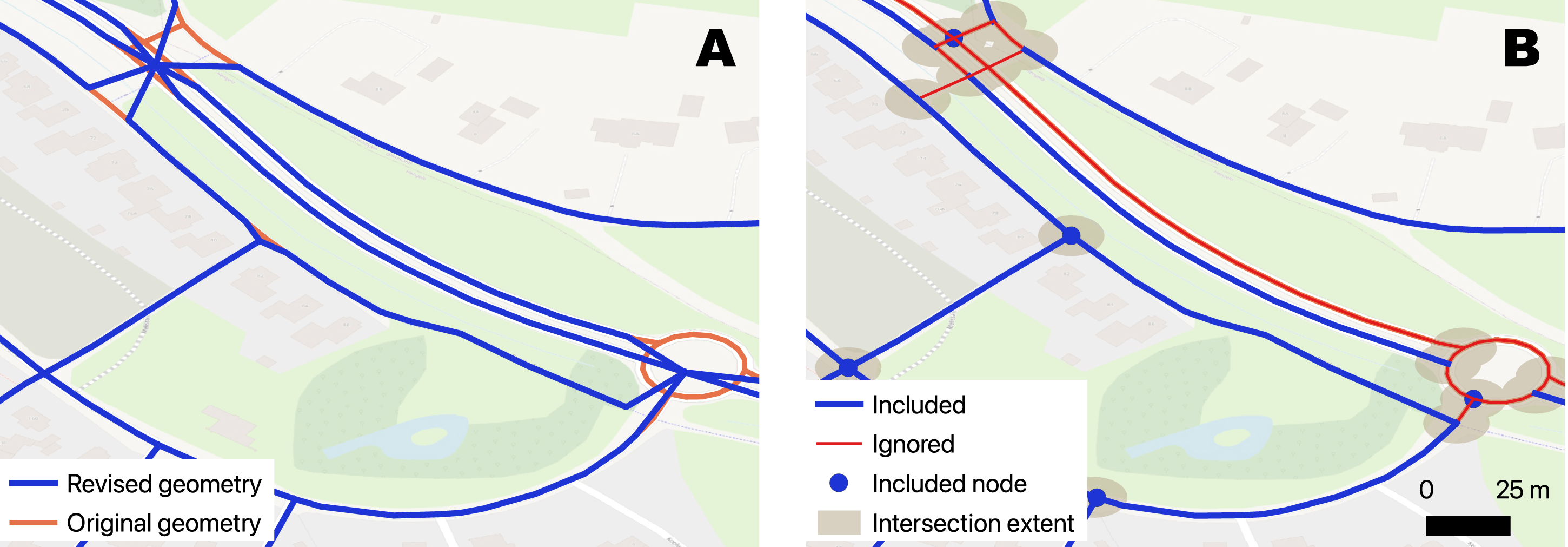

In the present analysis, we adopt an approach that preserves all original nodes and edges (summarized in Table A2). We identify clusters of nodes where each node is within 20 m (via the street network) of another node, and select a random node to represent that cluster (Figure 1, panel B). All other nodes are ignored at the later stage when we calculate aggregate connectivity measures, in order to avoid double weighting these intersections (Figure 2(A)) and to avoid inflating the nodal degree of these intersections (Figure 2(B)). Moreover, edges $<$ 20 m in length are classified as “intra-cluster,” and are also ignored in the aggregation. However, these intra-cluster nodes and edges are retained for purposes of calculating circuity—they can form part of the shortest path between two non-intra-cluster nodes (Figure 2(C)). In Figure 2, for example, the blue nodes would not even be connected without considering the intra-cluster and other ignored (red) edges.

Figure 2.

Rationale for excluding ignored nodes and edges from the aggregations (A, B, and D), although the ignored edges are considered when calculating circuity (C).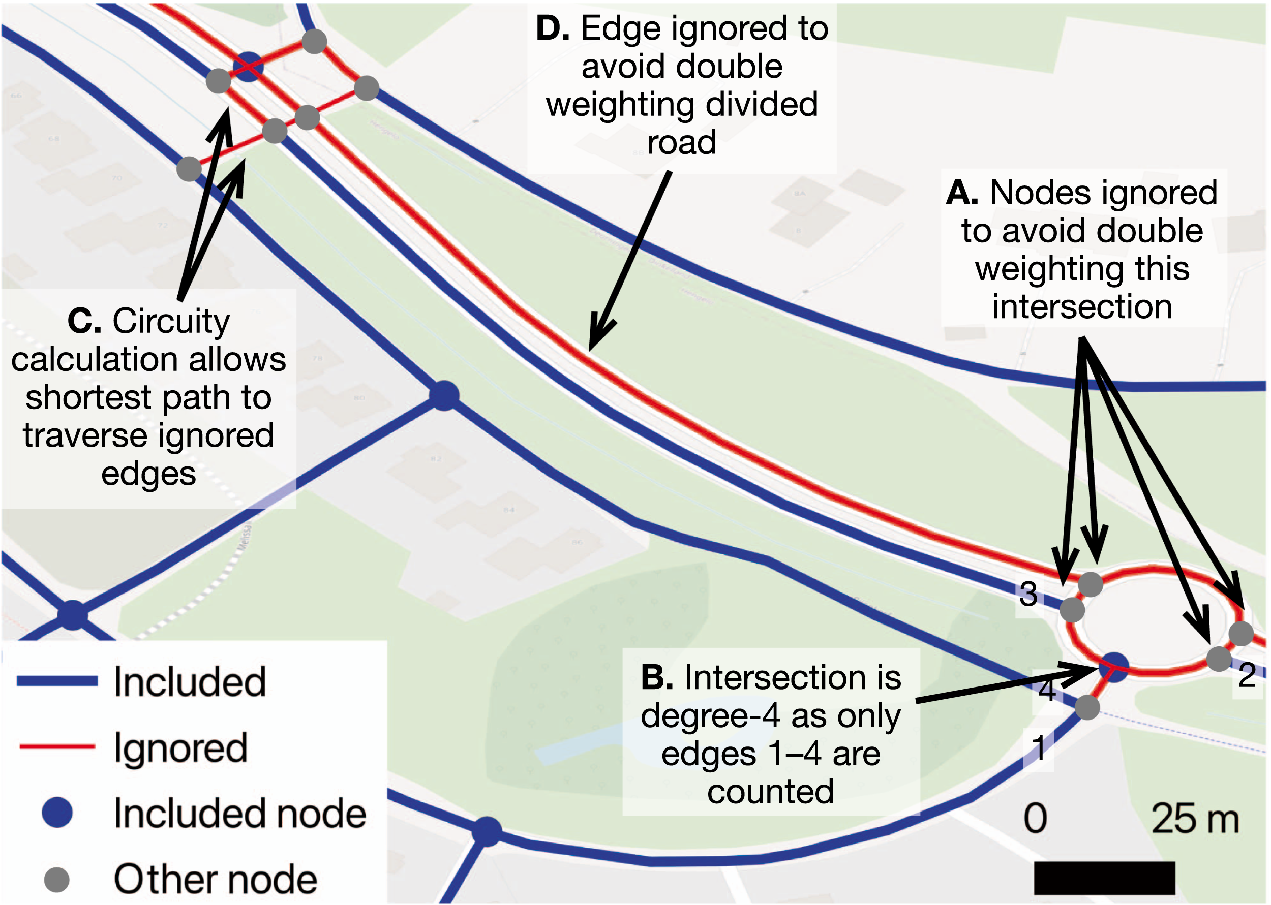

Divided roads

In some cases, roads with a center median are depicted as two parallel edges in OSM, even if they are functionally the same road. This would effectively mean that these roads are double-weighted in our calculations of SNDi. To mitigate this issue, we identify sets of two or more parallel edges, defined as those that start and end in the same two clusters of nodes. Within each set, we first drop footpaths, bicycle paths, and similar edges where there is a parallel “car” edge; typically, these are footways or bicycle paths alongside a road. Of the remaining edges in each set, we identify those that have the same name (e.g., “Main Street”) and randomly select one edge to represent the set. The remaining edge or, rarely, edges are retained for purposes of calculating circuity, but ignored for the aggregation (Figure 2(D)).

Overall, 8.0 million sets of parallel edges exist in our final dataset. Of the 17.7 million constituent edges, we tag 1.2 million as “ignore” because a parallel edge with the same OSM name exists.

As with many simplification algorithms, merging divided roads is a tradeoff between false positives (i.e., merging roads that are functionally separate) and false negatives (i.e., retaining two sides of a divided highway that are functionally a single road). It is also unclear where to set the dividing line—at what point do two parallel edges become functionally separate? Because we rely on heuristics and do not formally test the tradeoff, we err on the side of avoiding false positives by dropping only edges that meet both criteria (same OSM name and same start and end clusters of nodes). Thus, our approach improves on using the raw network, but does not address all cases of divided roads.

False negatives might arise where the name of an OSM way is missing or misspelled, or where the name differs between the two sides of a divided road. Spot inspections of a random sample of parallel edges suggests that where the OSM names differ, the edges are normally functionally separate (e.g., there are buildings between them) and using the OSM name is thus a useful discriminator. However, where the OSM name is missing (as is the case for 13.4 million parallel edges), more false negatives are likely to arise. The detailed algorithm (provided in the appendix) and our full code repository allow others to build on our work.

Other simplifications

As in our 2019 analysis, we drop duplicate geometries, and anneal degree-2 nodes, which by definition do not represent intersections. Their existence is an artefact of the import process or simply reflects the way data have been entered into OSM.

Simplification procedure

Because simplification can create further degree-2 nodes, we repeat certain steps of the process multiple times, as follows:

1. Create clusters: identify clusters of nodes where each node is within 20 m of at least one other node in that cluster.

2. Within each cluster, randomly select one node to represent the cluster. Other intra-cluster nodes are retained but ignored in the subsequent aggregation, as are edges that link nodes in the same cluster.

3. Anneal degree-2 clusters: if a cluster only has two edges that link it to nodes outside the cluster, then compute the shortest path across that cluster. Retain that shortest path and remove other intra-cluster edges.

4. Anneal nodes: delete degree-2 nodes, that is, any node that is neither a deadend nor an intersection.

5. Until no more changes are needed, repeat steps (1) through (4), as step (4) may have made some clusters smaller.

6. Drop footways and bicycle paths where they start and end in the same cluster as at least one other edge.

7. Anneal nodes, as step (6) may have created degree-2 nodes.

8. Identify and classify divided roads: where two or more edges start and end in the same cluster and have the same road name in OSM, randomly choose one of them to represent the road. Other edges are retained but ignored in the subsequent aggregation.

9. Anneal degree-2 clusters and anneal nodes as in steps (3) and (4) above, and repeat until no degree-2 nodes remain.

Computing connectivity measures

Detailed descriptions of the computation method for each connectivity measure from a network of nodes and edges are given in Barrington-Leigh and Millard-Ball (2019, Appendix A) and are unchanged. A summary table of the breadth and conceptual content of metrics is reproduced in Table A1.

Circuity correction

One change from our 2019 analysis relates to our circuity measures, which we compute for every node i for multiple distance bands (d₁, d₂). For each band (d₁, d₂), e.g., 500 m–1000 m, we calculate the sum of the Euclidean distances from node i to every other node that lies between Euclidean distances d₁ and d₂, and do the same for the network distances to every node in the same Euclidean distance band. We then calculate the log ratio of Euclidean to network distance. In our 2019 analysis, we simplified by excluding any node pairs greater than 3000 m apart via the network. This underestimated circuity, particularly for the higher distance bands. In the revised analysis, we relax this constraint to 5d₂ (e.g., 15 km for the 2500 m–3000 m band). Where the network distance is greater than 15 km or is not defined (as in an island with no road connection), we top-code it to 15 km for computational reasons.

Urban region and time series identification

Our primary results are restricted to urbanized areas. In our 2019 analysis, we used a custom classification of urban areas based on country-specific density thresholds. Since then, the release of the Global Human Settlements Layer (Pesaresi, 2023) provides a consistent typology of urban settlements across countries, using the EUROSTAT “degree of urbanization” classification. Therefore, we now use the GHSL data (2023 release of GHS-SMOD) to identify urban areas. Specifically, we identify an edge or node as “urban” if it intersects a pixel classified by GHSL as “urban center,” “dense urban cluster,” “semi-dense urban cluster,” or “suburban or peri-urban” (classes 30, 23, 22, and 21). The remaining classifications are various types of rural settlement.

We also use the GHSL data (specifically the 2023 GHS-BUILT-S raster) to develop a time series of street-network sprawl. Each GHS-BUILT pixel is classified as follows: land not built-up; built-up from 2005 to 2019 epochs; built-up from 1990 to 2004 epochs; built-up from 1975 to 1989 epochs; built-up before 1975 epoch. We calculate the built-up epoch based on when at least half of the ultimately developed pixels in the 100 m grid cell(s) that intersect each edge and node had been developed. For example, suppose that the intersecting grid cells have 20 pixels marked as developed by 1975, 60 by 1990, 70 by 2005, and 100 by 2020, with a further 50 pixels not built-up in any of these epochs. Then, we would assign an epoch of 1975–89, as more than half of the built-up pixels (60/100) had been developed by 1990.

Aggregation

We aggregate to a 1 km grid and to the administrative areas (countries and up to 5 subnational levels) demarcated in the Global Administrative Areas (GADM) dataset.

As in our 2019 analysis, we allow footpaths, bicycle paths, service roads, and similar edges to contribute to the connectivity of the network, but do not consider these nodes and edges in our aggregation, or as origins or destinations in the circuity analysis. This exclusion helps to avoid several potential biases. For example, the “service” tag is often used to identify private driveways, a practice that would inflate the fraction of dead ends. “Service” tags also represent other access roads that do not form part of the public street network, and aisles in parking lots, the internal connectivity of which has little relevance to urban form or travel behavior. The same is true for networks of walking paths in public parks, which can be represented in minimal or excruciating detail depending on the OSM contributor.

Even though these footpaths, bicycle paths, and service roads are excluded from the aggregation, they are included when computing graph properties and our measures of dendricity, nodal degree, and circuity. Inclusion of these edges markedly increases connectivity in places such as Denmark, where residential streets are often designed as deadends for cars but allow pedestrians and bicyclists to continue through. Thus, even though they are not included in our aggregates, pedestrian and cycle paths improve the measured connectivity of nearby streets.

Results

The upper panel of Figure 3 shows SNDi at the country level for the entire stock of streets represented in OpenStreetMap. Countries with more connected streets (lower SNDi) are in blue, and those with higher SNDi in red. Connectivity is highest in much of South America (especially Argentina), continental Europe, North Africa, and parts of East Asia, especially Japan, South Korea, and Taiwan. At the other extreme, while the United States is the poster child for car-dependent suburban development, street connectivity is even lower (higher SNDi) in south and southeast Asia, particularly Thailand and Bangladesh.

Figure 3.

Upper panel: street-network sprawl (SNDi) for the stock of streets, 2023. The inset shows the distribution (kernel density) of SNDi for 1 km² grid cells in the five most populous countries. Lower panel: SNDi for streets developed in 2005–19. The inset shows how the distributions at the grid cell level (measured via kernel density) have shifted out over our four epochs, marking the shift toward less-connected streets over time.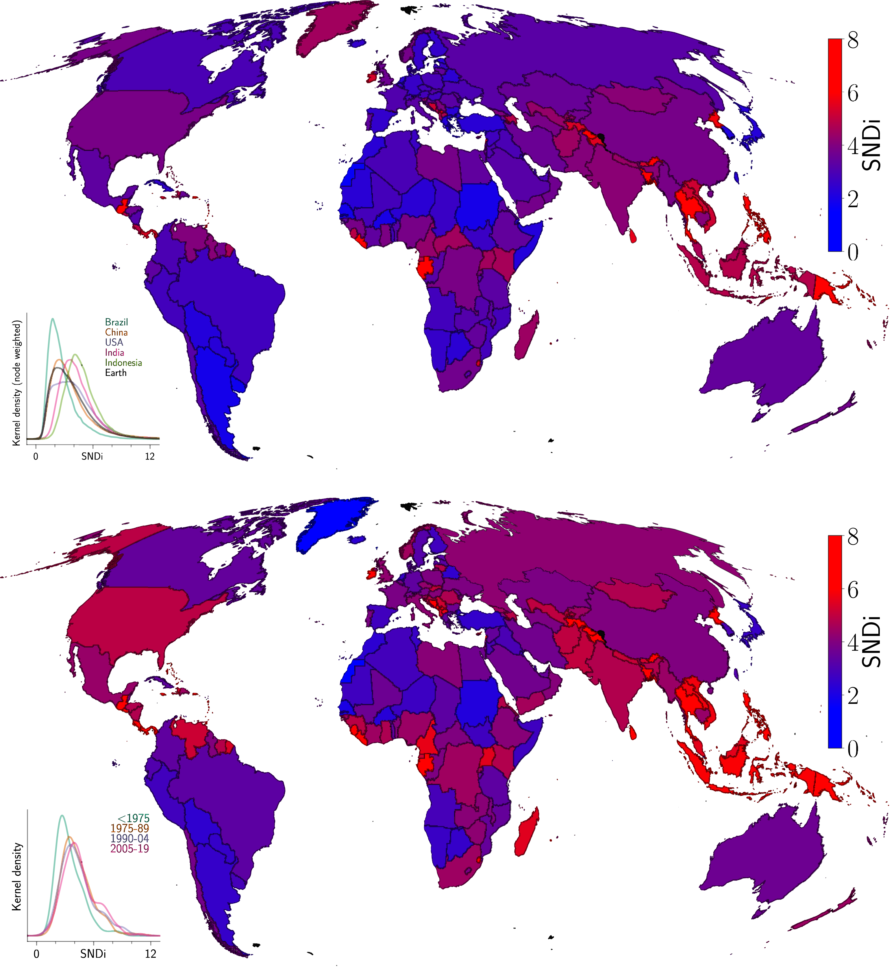

The global differences in street connectivity are even more marked when considering streets constructed in the most recent of our four epochs, 2005–19 (Figure 3, lower panel). Southeast Asia, including Indonesia and the Philippines, is particularly notable for its high levels of SNDi in recent construction.

Within-country variation is also noticeable. In addition to the downloadable data, our companion website at https://sprawlmap.org provides interactive maps of our results aggregated to five levels of subnational administrative geographies and to a 1 km grid.

Figure 4 shows trends in SNDi over the full range of our time series. In panels A and B, we have aggregated new development in urban areas across countries according to World Bank geographic and economic groupings. Many features are qualitatively consistent with our earlier work. However, updating the data to more recent years shows a generally steeper increase in street-network sprawl in most regions and overall across Earth. Panel C shows trends aggregated to the country level for large countries, while panel D presents trends for large cities, but using a different time series which specifies urban development boundaries up to 2013 (Angel et al., 2012, 2016). While our previous work suggested that SNDi had plateaued in a number of locations and regions shown in Figure 4, the updated analysis provides instead a picture of increasingly disconnected development in the largest cities and generally in developing and middle income countries.

Figure 4.

Trends in SNDi over time at the regional level (A), by the World Bank’s country development classification (B), for a selection of large countries (C), and for a selection of large cities (D). HIPC is the World Bank’s heavily indebted poor country category. While trends show SNDi of new development during each time period, the solid circles show SNDi of the stock of all streets.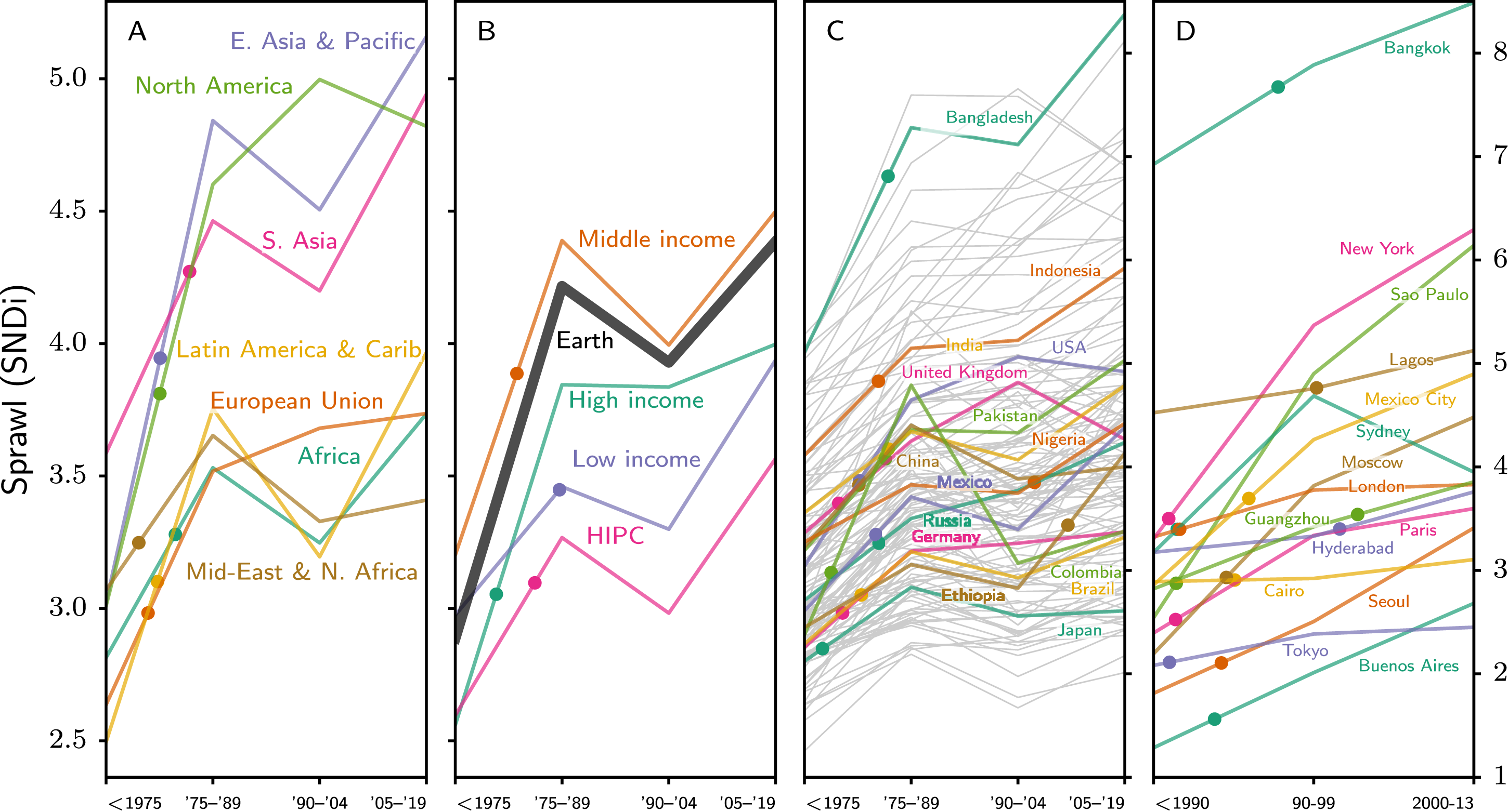

Even though the main feature of our new analysis is that the data are available at a highly disaggregated level, allowing for a variety of more detailed analysis, we provide one more example of high-level aggregation to extend the city-level picture. Figure 5 shows the average SNDi over the stock of streets in 2013 for a number of large cities, as well as that of new development in the 2000–2013 period. Patterns generally match the country-level picture of Figure 3.

Figure 5.

Distribution of SNDi for major cities in 2013 (top) and in recent development (bottom).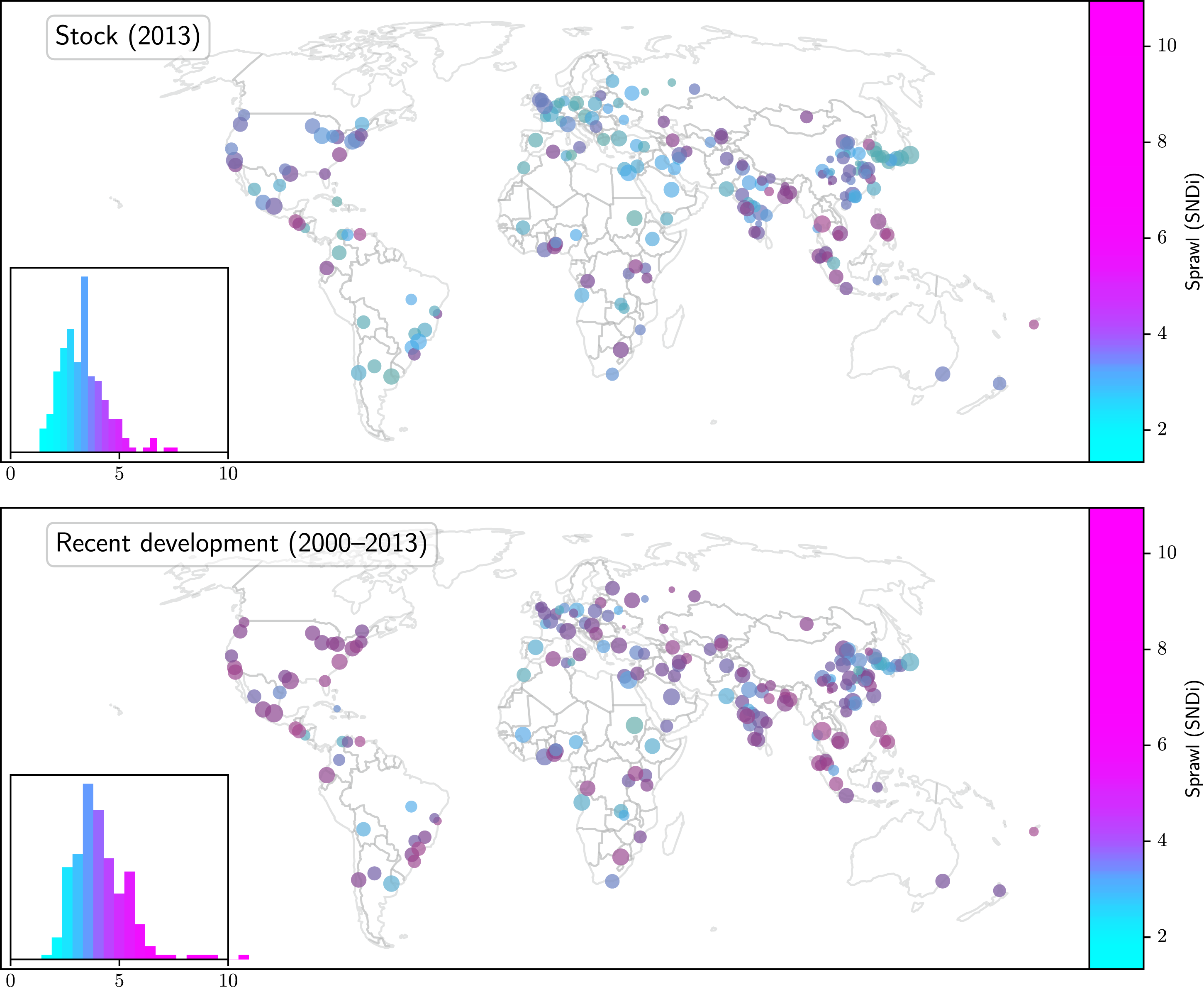

Data and code availability

Our analyses are available under a CC BY 4.0 License in three general geospatial formats:

1. as gridded data, specifying SNDi and its component metrics at 1 km resolution,

2. as vector polygon data, aggregated to geopolitical boundaries at several spatial scales, using the Global Administrative Areas v4.1 dataset (GADM, 2022), from nodes and edges characterized as urban,

3. and as vector network data, specifying each node and edge and its characteristics.

Our provision of the underlying vector network data facilitates the creation of more detailed time series for specific locales. For instance, while our work relies on the GHSL in order to provide global coverage, data available for specific countries or metropolitan areas may offer higher temporal resolution (e.g., Barrington-Leigh and Millard-Ball, 2015; Turner et al., 2023).

The data are hosted by OSF at https://osf.io/c9hjy.

We also provide our code as an open GitLab repository at https://gitlab.com/cpbl/global-street-network-sprawl-sndi. Given the hardware requirements and computation time, we suggest that our pre-prepared data products will be more valuable for most users. However, the code enables researchers to build on our algorithms and explore other extensions.

Conclusion

Our release of these analyses is intended to facilitate further exploration of patterns and trends in important characteristics of street networks worldwide. By releasing both spatially aggregated data and the underlying network layer, and both the SNDi and its component metrics, we hope to offer convenience and ease for moving beyond a simplistic and Americas-centric approach to quantifying street-network connectivity. SNDi can serve as a point of comparison which has been validated across different historical development forms, and which detects stark and regionally differentiated trends over recent decades. By providing a 45-year time series, we hope to facilitate studies of street connectivity that move beyond the descriptive to examine the causal role of streets in shaping economic, social, and environmental outcomes.

Supplemental Material

Supplemental Material - A high-resolution global time series of street-network sprawl

Supplemental Material for A high-resolution global time series of street-network sprawl by Christopher Barrington-Leigh and Adam Millard-Ball in Environment and Planning B: Urban Analytics and City Science.