Sage Journals: Discover world-class research

Abstract

The performance of Land Use Change (LUC) models is influenced by the regional spatial characteristics that trigger the changes. However, the literature on LUC models generally reports validation results for entire regions without considering subregions that differ significantly in their LUC drivers. This research explores how the LUC driving forces differ among subregions and whether regionalization can improve the performance of LUC models in areas undergoing rapid urbanization. We analyzed the Geomod, Cellular Automata-Markov, and Land Change Modeler models across rural and urbanized subregions on the western edge of Mexico City. Regionalization significantly enhanced the overall accuracy of the models and the concordance of spatial patterns with the reference data in rural regions but was of limited benefit in urbanized regions. This shows the need to consider regionalized modeling to improve the performance of LUC models when there are noticeable differences in LUC drivers between subregions. These findings will enhance the usefulness of LUC models for urban planning and land management policies, promoting more precise and effective decision-making.

Keywords

Land-use and cover change modeling validation model performance urban growth

Introduction

Spatially explicit Land Use Change (LUC) modeling has contributed to territorial planning by predicting the change and spatial distribution of land uses (Heidarlou et al., 2019; Ren et al., 2019; Wang et al., 2023). The models can also help to build future land-use change scenarios according to a given social and ecological environment (Lopes et al., 2023; Seevarethnam et al., 2022). However, the model’s output must correspond to real-world behavior before it can lead to well-founded decision-making (Aguejdad et al., 2017; Di Lucia et al., 2021; Lü et al., 2020; Saltelli and Funtowicz, 2014); crucially, the predictions of LUC models are sometimes inaccurate (Brown et al., 2013) because of the complex dynamics of land-use change, which involves biophysical processes and human decisions. Thus, it is essential to assess the performance of LUC models (the agreement between observed and predicted land use) (Amiri et al., 2017; Dezhkam et al., 2017; Paegelow et al., 2014). For this assessment to be accurate, it is necessary to consider the main drivers of land use and land cover change: socioeconomic factors, proximity, site factors, and planning and policy (Camacho, 2022; Naikoo et al., 2022); these can significantly differ amongst subregions, driving diverse LUC behaviors (Yang et al., 2014). For instance, it has been reported that urban expansion generally occurs around pre-existing urban areas (Pribadi and Pauleit, 2015; Tian, 2015; Winarso et al., 2015) and not in areas far from them. Linked with this is that areas with higher population densities generally have more dynamic land use changes due to more economic and social incentives for development (Gomes, 2020). Proximity to roads also triggers land use change by facilitating resource access for people while the change decreases with increasing slope (Arfasa et al., 2023). Despite the differences in land-use change dynamics between subregions, many studies do not consider differences between subregions and the effects that these may have on the performance of a model (Kumar et al., 2016; Sakieh and Salmanmahiny, 2016; Subedi et al., 2013; Yang et al., 2014). For instance, a model developed for a large area might assume uniformity in factors such as agricultural practices, urbanization rates, or conservation policies, whereas these may differ significantly across smaller regions (Brown et al., 2013). This can lead to less accurate or less applicable results for specific subregions. Focusing on smaller subregions allows researchers to capture the nuances and local variations in land-use changes that might be averaged out or overlooked in a study across a larger area. These variations can include specific socioeconomic and biophysical drivers critical for a more granular understanding and prediction of land-use dynamics (Gaur and Singh, 2023). Owing to this spatial non-stationarity of land use change, it is essential to assess which model best fits the actual trends in each subregion. Regionalization, that is, grouping locations with similar characteristics into the same subregion, can help to account for spatial non-stationarity (Verburg et al., 2002); it can capture the behaviors in each subregion, thus improving a model’s accuracy (Briassoulis, 2020).

Comparison of the performance of models can help to identify which model(s) provide(s) the best predictions for a subregion or an entire area. It may be possible that those models that include the socioeconomic and biophysical drivers of land-use change in their algorithms might capture more appropriately the particular land-use process in a subregion, leading to higher performance than those models that rely solely on the previous land-use state and the state of the neighboring area. Therefore, this article aims to evaluate how subregional spatial characteristics influence the performance of Land Use Change (LUC) models by focusing on two contrasting subregions: urbanized (built-up land) and rural (agricultural land and natural vegetation), in an area of rapid urban growth in the western part of Mexico City. It compares the performance, with and without regionalization, of three of the most widely used LUC models applied in different contexts around the world: Geomod (Cruz-Bello et al., 2023; Mirzapour et al., 2020; Nahib et al., 2018; Sakieh and Salmanmahiny, 2016; Shade and Kremer, 2019), Cellular Automata Markov (Amiri et al., 2017; Dezhkam et al., 2017; García-Álvarez et al., 2019; Khwarahm et al., 2021; Seevarethnam et al., 2022), and Land Change Modeler (Aguejdad et al., 2017; Camacho et al., 2015; García-Álvarez et al., 2019; Shade and Kremer, 2019; Shooshtari and Gholamalifard, 2015). The aim is to improve the predictive accuracy of Land Use Change models by accounting for regional differences, which will enhance their usefulness for planning and policy-making in rapidly urbanizing areas.

Materials and methods

Study area

The study area encompassed 30,801 hectares within three municipalities of western Mexico City (Huixquilucan de Degollado, Cuajimalpa de Morelos, and Álvaro Obregón) (Figure 1). We recognized two subregions, urbanized and rural, according to the classification into basic geostatistical areas (AGEBs), which are the smallest geographic units used by the geography and statistics agency of the Mexican government (INEGI, 2014). An urban AGEB is an area between 1 and 50 blocks delimited by streets, avenues, and walkways, with land use mainly residential, industrial, service, or commercial. A rural AGEB is in rural areas with variable sizes characterized by agricultural or forest land use and rural localities (INEGI, 2010, 2020). This regionalization omits the peri-urban transition zones between rural and urban areas, the delimitation of which is still a topic of research (González-Arellano et al., 2021). In the urbanized subregion (urban AGEBs), which covered 14,510 ha, the population density is 149.5 inhabitants per hectare and the road density 285 m/ha. In the rural subregion (rural AGEBs), which comprised 16,291 ha, the population density is 20.5 inhabitants per hectare and the road density 178 m/ha. The densities were calculated using data from INEGI (2010, 2015).

Figure 1.

Study area. Urbanized and rural subregions on the western edge of Mexico City.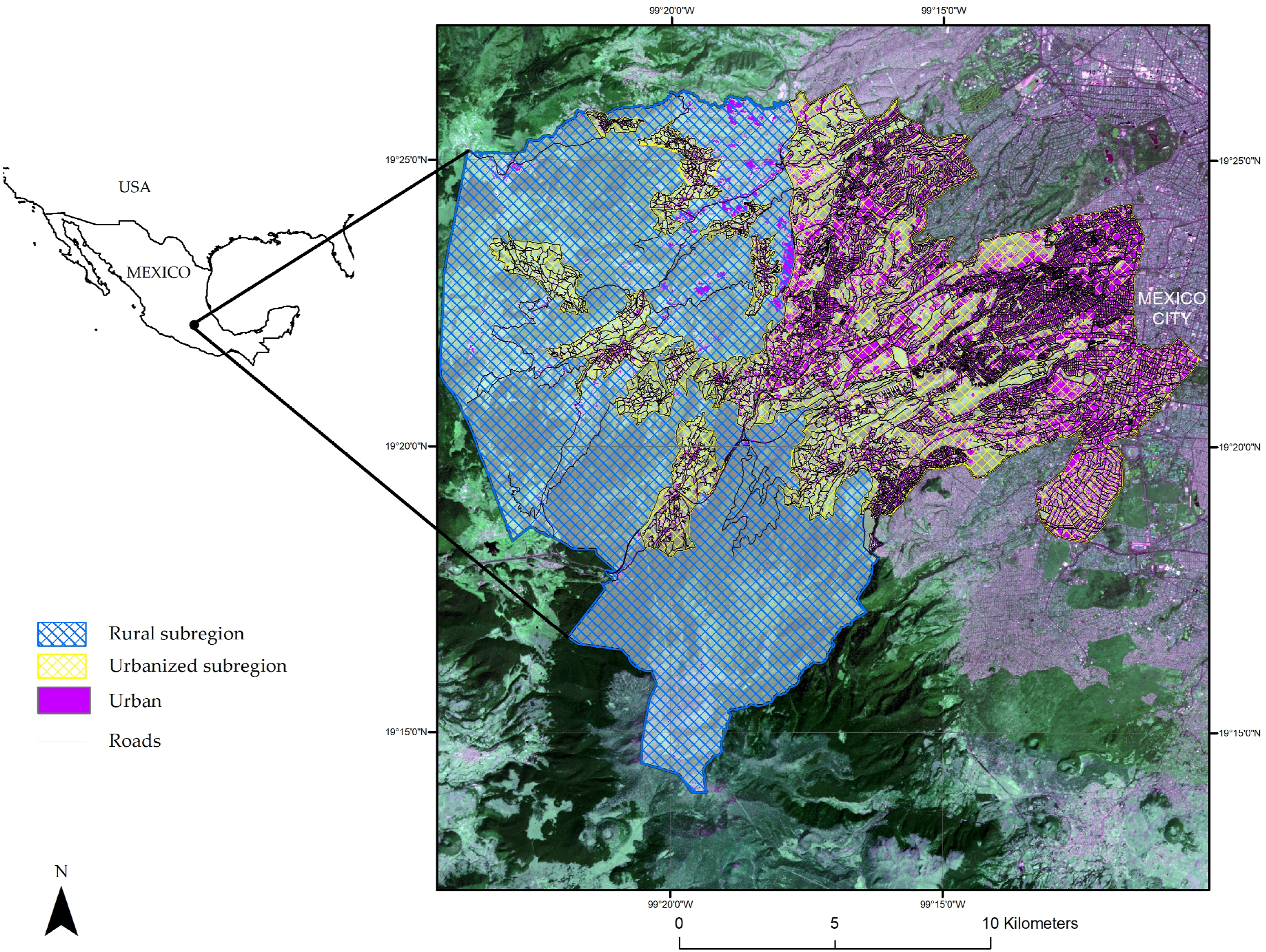

Methods

Driving forces selection and comparison

To verify that these subregions differ in the values of the possible LUC drivers, we selected from the specialized literature some of the most frequently reported drivers (Aguejdad et al., 2017; Ahmed and Ahmed 2012; Amiri et al., 2017; Arfasa et al., 2023; Camacho, 2022; Cruz-Bello et al., 2023; de Souza et al., 2022; García-Álvarez et al., 2019; Mirzapour et al., 2020; Mohamed and Worku 2020; Seevarethnam et al., 2022; Shade and Kremer, 2019). To look for distinct patterns for the driver in the two subregions, indicating differences in its distribution, we generated and compared the histograms of the following variables for each subregion: Distance to roads (m) (INEGI, 2015); Protected Areas (presence) (CONANP, 2015); Distance to urban areas (m); Population density (persons per hectare) (INEGI, 2010); Elevation (m a.s.l.) (INEGI, 2013); Slope (%); and Land-use. The same interval was used for each variable in both subregions. To confirm that driver distributions in the two subregions are significantly different, we performed a Chi-square test for each variable to compare the frequency distribution.

Using Cramer´s V statistic, we assessed the relationship between drivers and LUC; this statistic measures association, where 0 indicates no association, and 1 indicates a perfect relationship (Subiyanto and Suprayogi, 2019). Figure 2 illustrates a methodological flowchart of the activities involved in the study.

Figure 2.

Methodological flowchart.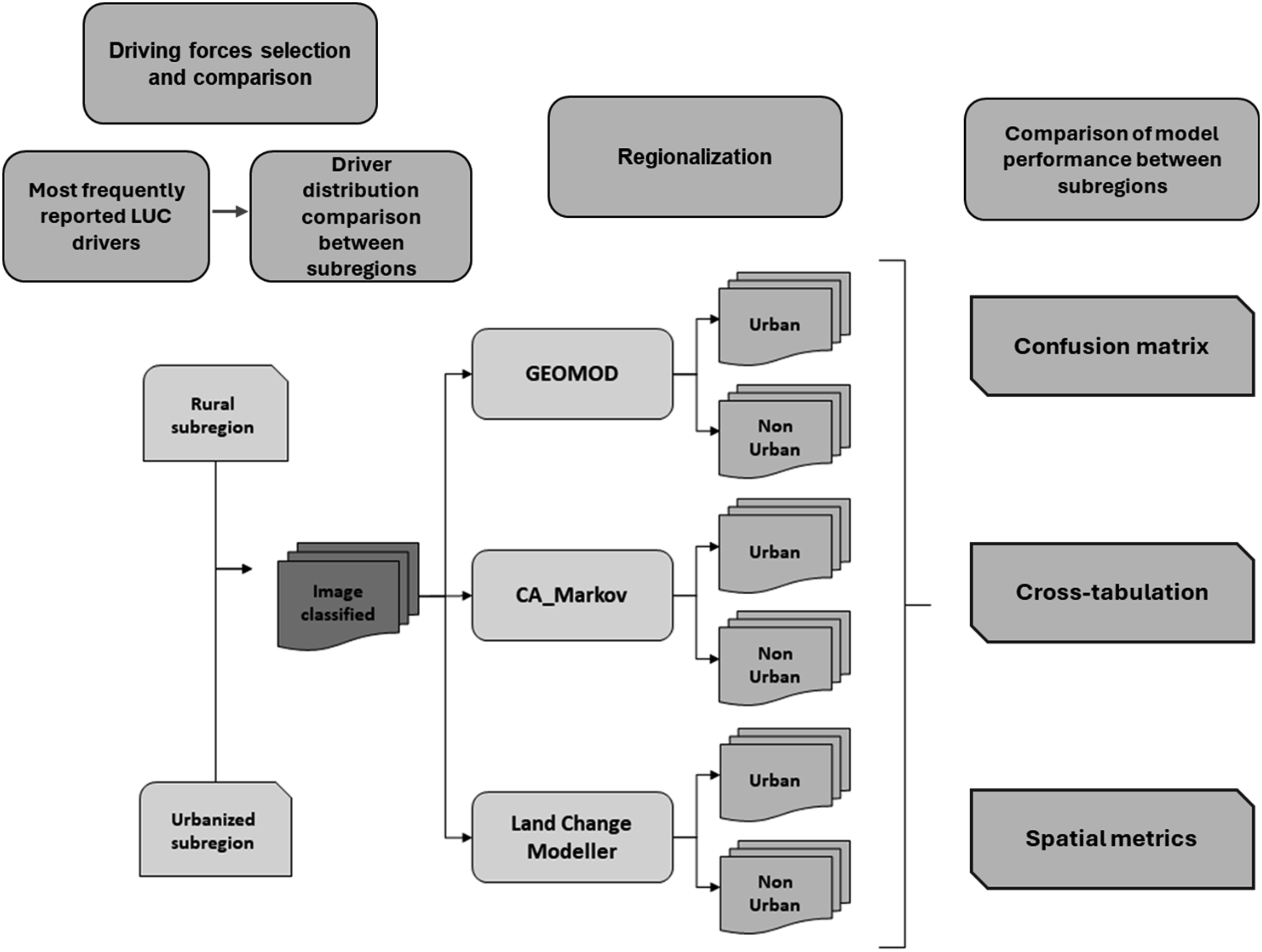

Land-use analysis

Analysis of land-use change from non-urban to urban in each subregion used SPOT 5 satellite images of the dry season (November – December) of 2005, 2010, and 2014 (SIAP, 2017). A supervised classification was performed using the maximum likelihood method in Terr Set software; the total accuracy of the classifications surpassed 90%, which complies with specialized literature standards (Islam et al., 2018; Pontius, 2019). The analysis showed an increment in urban area in each subregion: in the urbanized subregion, the urban class increased from 37.5% of the study area in 2005 to 43.3% in 2010 and 58.4% in 2014; in the rural subregion, the urban class increased from 1.2% in 2005 to 2.4% in 2010 and almost 8% in 2014.

Land-use change modeling

To compare the performance of the LUC models in different subregions, the change predictions from non-urban to urban during 2010–2014 were separately modeled and validated for the entire region, the urbanized subregion, and the rural subregion. Land-use images from 2005 and 2010 were set as the earlier and later dates, to predict urban areas in 2014. Three widely used models were applied: Geomod, CA_Markov, and Land Change Modeler (LCM), all available in the TerrSet software. The spatial resolution of the land use and the LUC driver layers was 10 m, the original resolution of the SPOT images obtained from SIAP (2017). Detailed information on each LUC model’s characteristics and calibration is provided in Supplemental Material.

For Geomod, the layer of land suitability for urbanization that this model requires was generated by following the specialized literature that reported several urban growth drivers (Nahib et al., 2018; Shade and Kremer, 2019). For this study, we used distance to roads, elevation, slope, population density, protected areas, distance to urban areas, and the land use class (agriculture, forest, urban) of 2005 (analysis beginning date). We used the unconstrained neighborhood search mode to select change locations, which allows the change to happen in any pixel. Linear models were generated with data from 2005 and 2010 to estimate the urban area in 2014.

Regarding Cellular Automata Markov (CA_Markov), the transition probability matrix from non-urban to urban was calculated using a proportional error of 10 for 2005–2010. Then, the land suitability for each land-use class was determined considering that areas near an existing land-use class are more likely to change into that class than areas far from that class. Therefore, the Euclidean distance to each land-use class was calculated, and a monotonically decreasing J-shaped fuzzy membership function was applied to define the relative suitability for the two land uses (Subedi et al., 2013). Ten cellular automata iterations were used, and a 5 x 5-contiguity filter was used for each run.

In the case of the Land Change Modeler (LCM) a logistic regression analysis was used to predict change from non-urban to urban land use. The transition potential layer from non-urban to urban was created by analyzing the transition potential layer (2005–2010) and the same land-use change variables (drivers) used to generate the land suitability layer in Geomod. The Cramer’s V index was used to measure the explanatory power of each variable in the land-use change (Eastman, 2016). We considered a Cramer’s V threshold value of 0.15 (Ahmed and Ahmed, 2012; Shooshtari and Gholamalifard, 2015). All variables exceeded this value. Thus, they were judged to be associated with a particular type of land use and included in the logistic regression analysis to predict a change from non-urban to urban use, where a 10% stratified random sampling was applied.

Comparison of model performance between subregions

We compared each model’s performance between the two subregions, evaluating the concordance between each model’s prediction for the urbanized, rural, and total area against the reference data (SPOT classification 2014). First, we compared the area percentage of each land-use class and generated confusion matrixes to assess the correspondence between modeled and observed data. This determined the agreement between the model’s prediction and the reference data regarding the area and the geographical location.

Second, to eliminate that part of the prediction’s accuracy that is attributable to land persistence, we applied a cross-tabulation technique (Paegelow et al., 2022; Pontius et al., 2008) overlaying the land-use map 2010, the reference map 2014, and the predicted map 2014. This analysis was implemented for the total area and each subregion using the LCM verification module. A layer with four validation categories was generated: (1) Correct rejection (LU persistence was predicted, and it persisted); (2) Hit (LU change was predicted, and it changed; (3) False alarm (LU change was predicted, but it persisted); and (4) Failure (LU persistence was predicted, but it changed) (Eastman, 2016).

A Chi-square test assessed the relationship between subregions and validation categories by observing statistically significant differences in each model’s performance depending on the subregion (Agresti, 2007). The Chi-square test is commonly used in Land Use Change analysis to determine whether the observed changes are significantly related to a given condition (Malaki et al., 2017). Also, standardized residuals were computed to locate the combination subregion-validation category where significant differences in the model’s performance were present.

Third, a pattern accuracy metric evaluation was carried out (in other contexts also called landscape accuracy metric evaluation). A series of spatial metrics were used, independently for each model and subregion, to assess the correspondence between the modeled spatial patterns of urban land use—including arrangement, fragmentation, and core areas—and their actual patterns in reference maps (Teimouri et al., 2023). Following Sakieh and Salmanmahiny (2016), the metrics were Class Area (CA), Percentage of Landscape (PLAND), Number of Patches (NP), Patch Density (PD), Largest Patch Index (LPI), Total Edge (TE), Edge Density (ED), Largest Shape index (LSI) and Mean Euclidean nearest neighbor distance (ENN_MN) (Table S1); these metrics were computed with FRAGSTATS 4.2.1 software (McGarigal et al., 2012)

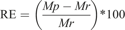
To evaluate the accuracy of Land Use Change modeling by comparing the metrics derived from the modeled and reference layers (Dezhkam et al., 2017), we computed the Relative Error (RE) and Mean Relative Error (MRE). The Relative Error (RE) measure allows comparison across different regions or scenarios (Foody, 2010). It measures the difference between the modeled and reference layers divided by the reference layer

RE = (\frac{M p - M r}{M r}) * 100

where M_p and M_r are the values of the spatial metrics from the modeled and reference LUC layers, respectively.

The Mean Relative Error (MRE) is the Relative Error average across all pixels or regions. It summarizes the modeled layer’s overall accuracy in matching the reference layer (Burnicki et al., 2007)

MRE = \frac{1}{n} \sum_{i = 1}^{n} {RE}_{i}

where RE_i is the absolute Relative Error of the model output for the i LUC for each spatial metric; n is the number of estimated relative errors.

The absolute value of the Relative Error was classified by the level of agreement of the metrics between the simulated and the reference maps: 0–15 High, 15–30 Good, 30–45 Average, and >45 Low (Dezhkam et al., 2017).

Results

The histogram comparisons revealed distinct patterns in the distribution of LUC driver values between rural and urbanized subregions (Figure 3). The urbanized subregion showed areas generally closer to roads, while the rural subregion had larger distances, indicative of less developed areas. Protected areas were present in both subregions, but the rural subregion had a higher concentration, while the urbanized subregion had fewer protected areas. As could be expected, the urbanized subregion was located nearer to urban centers, in contrast to the rural subregion’s wider spread of distances from urban centers. Population density was significantly higher in the urbanized subregion, reflecting a more densely populated area compared to the rural subregion’s lower densities. The elevation histograms revealed that the rural subregion covered diverse altitudes, while the urbanized subregion was more concentrated at lower elevations. The rural subregion also showed greater variability in slope, with steeper areas being more common. In contrast, the urbanized subregion had a narrower distribution, with less steep slopes. Land-use patterns differed, with the urbanized subregion having a higher frequency of built-up areas. In contrast, the rural subregion showed more agricultural and natural land uses, consistent with its lower population density and greater distance from urban centers (Figure 3). These differences were statistically significant, Chi-square; p < .001 for each LUC driver, confirming distinct patterns in the driver distributions between the two subregions.

Figure 3.

Values of each LUC driver for the urbanized and rural subregions.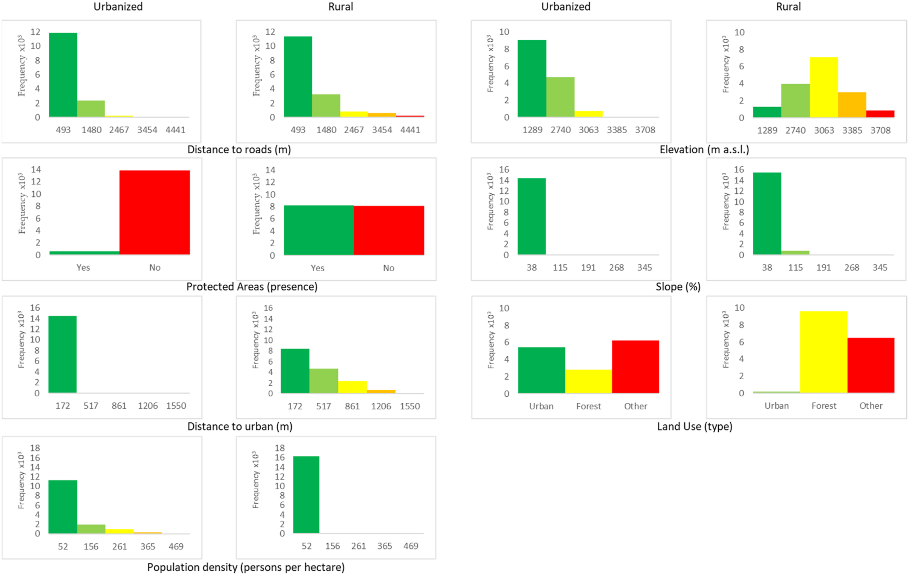

According to the Cramer V statistic, the most critical LUC driver for the total area was elevation (0.54), followed by distance to urban areas (0.52) and population density (0.42). For the urban and rural regions, the most critical driver was the distance to urban areas (0.54, 0.43), followed by elevation (0.34, 0.26) and population density (0.29, 0.20).

Comparison of model performance between subregions

Comparison to the reference data showed that Geomod had a greater underestimation of the urban class in the urbanized subregion than in the rural subregion. CA_Markov underestimated the urban area in the urbanized subregion but overestimated it in the rural subregion. LCM underestimated the urban class area in both subregions but more significantly in the urbanized subregion than in the rural one (Table S2; Figure S1). Comparison to the reference data showed that there was more underestimation of the urban area predicted by any of the three models in the urbanized subregion than in the total area. In the case of the urban area modeled by Geomod and LCM in the rural subregion, there was less underestimation than in the total area (Table S2; Figure S1); hence, for these models, regionalization improves the performance, whereas this was not the case for CA_Markov.

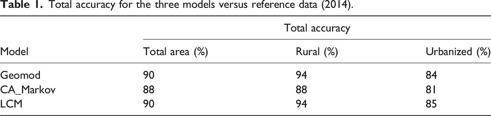
The confusion matrices generated to evaluate the correspondence between modeled and reference data revealed that in all models, the total accuracy was highest for the rural subregion, followed by the total area and the urbanized subregion (Table 1).

Table 1.

Total accuracy for the three models versus reference data (2014).

Model	Total accuracy
Model	Total area (%)	Rural (%)	Urbanized (%)
Geomod	90	94	84
CA_Markov	88	88	81
LCM	90	94	85

Cross-tabulation showed that, in each model, the rural subregion showed the highest percentage of persistence, followed by the total area and the urbanized subregion. In terms of Hits (the model predicted change, and it changed), the urbanized subregion had the highest percentages, followed by the total area and the rural subregion. For Misses (the model predicted persistence, but it changed) and False alarms (the model predicted change, but it persisted), the rural subregion had the lowest percentages, the urbanized region the highest, with intermediate percentages in the total area (Table 2). This result does not show a clear improvement if the modeling were to be regionalized.

Table 2.

Areas of the validation categories for the total area and the urbanized and rural subregions.

	Validation category
Subregion	Persistence (ha)	%	Hits (ha)	%	Misses (ha)	%	False alarms (ha)	%
Geomod
Rural	15,271	93.7	24	0.1	867	5.3	129	0.8
Urbanized	11,933	82.2	287	2.0	1896	13.1	394	2.7
Total area	27,272	88.5	378	1.2	2695	8.7	457	1.5
CA_Markov
Rural	14,008	86.0	311	1.9	579	3.6	1393	8.5
Urbanized	11,673	80.4	659	4.5	1524	10.5	655	4.5
Total area	26,210	85.1	1272	4.1	1801	5.8	1518	4.9
LCM
Rural	15,285	93.8	34	0.2	856	5.3	116	0.7
Urbanized	11,988	82.6	284	2.0	1899	13.1	340	2.3
Total area	27,337	88.8	410	1.3	2663	8.6	392	1.3

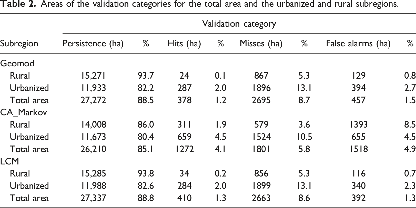
There was a strong dependency (Chi-square test; p < .0001) between the subregion (urbanized or rural) and the validation category (persistence, hit, miss, false alarm). Hence, the performance of each model differed significantly between subregions. The standardized residuals showed that the differences in model performance between subregions were mainly due to more persistence than expected in the rural subregion and less persistence than expected in the urbanized subregion for Geomod and LCM, and to fewer misses than expected in the rural subregion, and more misses than expected in the urbanized subregion for CA_Markov (Table S3).

The evaluation of the accuracy through spatial metrics in the urban class showed that when Geomod was regionalized, the number of patches was closer to the reference data in each subregion. When LCM and CA_Markov were regionalized, only in the rural subregion was the difference from the reference data in the number of patches reduced. For ED and LSI in the urban class, when Geomod and LCM were regionalized, the values of these indices were closer to the reference data only for the rural region; when CA_Markov was regionalized, the difference from the reference data occurred only for ED and only in the rural region. For ENN_MN in the urban class, in none of the models was the difference from the reference data reduced by regionalization (Table S4).

For the spatial metrics assessment, the performance of Geomod and LCM for the urban class was better in the urbanized subregion than in the rural subregion in terms of agreement with reference data. For CA_Markov, the levels of agreement did not differ between subregions (Tables 3 and S5).

Table 3.

Level of agreement between the simulated and reference data for each land use, subregion, and model. Nu, non-urban; U, urban.

Subregion	Land use	NP	ED	LSI	ENN_MN
Geomod
Rural	Nu	Low [−47.5]	Average [−42.9]	Low [−52.9]	High [0]
Rural	U	Low [−50.2]	Low [−57.1]	Average [−33.9]	Good [19.4]
Urbanized	Nu	Average [−36.8]	High [1.6]	High [−13]	High [-10.7]
Urbanized	U	Average [44.9]	High [−1.6]	High [6]	High [0]
Total area	Nu	Average [−33.5]	Good [−19.3]	Good [−24.2]	High [-10.7]
Total area	U	Good [−16.7]	Good [−19.3]	High [−9.7]	High [0]
CA_Markov
Rural	Nu	High [−14.3]	Low [−71.4]	Low [−64.7]	High [-4]
Rural	U	Low [−95.9]	Low [−71.4]	Low [−75]	Low [277.8]
Urbanized	Nu	Low [−94.2]	Low [−70.5]	Low [−71.2]	\|Low [103.6]
Urbanized	U	Low [−82.7]	Low [−70.5]	Low [−67.2]	Low [137]
Total area	Nu	Low [−93.4]	Low [−74.7]	Low [−73.7]	Low [96.4]
Total area	U	Low [−93.1]	Low [−74.7]	Low [−73.8]	Low [103.1]
LCM
Rural	Nu	Low [−55.4]	Low [−66.7]	Low [−58.8]	High [-4]
Rural	U	Low [−61.2]	Low [−66.7]	Low [−46.2]	Good [27.8]
Urbanized	Nu	Low [−48.3]	High [−14.7]	Good [−23]	High [0]
Urbanized	U	Average [31.9]	High [−14.8]	High [−6]	High [3.7]
Total area	Nu	Low [−62.3]	Average [−34.9]	Average [−37.4]	High [0]
Total area	U	Good [−19.9]	Average [−34.9]	Good [−24.8]	High [0]

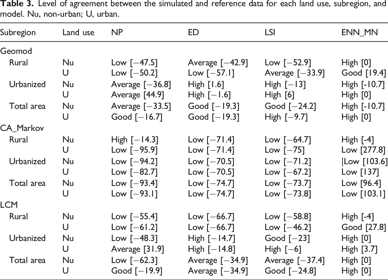
When comparing the levels of agreement between the total area and each of the subregions, the results are diverse for Geomod and LCM. For example, if we regionalize the modeling, in some cases the level of agreement increases, as in the urbanized subregion for ED. At the same time, for NP, it does not improve in any case for the urban class (Tables 3 and S5). For CA_Markov, regionalizing does not improve the urban class’s agreement level (Tables 3 and S5).

Discussion

The study showed significant differences in drivers of land use change between subregions, which was also reported by Ustaoglu and Aydınoglu (2019) for metropolitan regions in Turkey. The drivers that most influenced the land use change in our study area were the site factors (elevation), followed by proximity (distance to urban areas), and socioeconomic factors (population density). These results contrast with other studies of the Mexico City periphery. For example, in the city’s industrial area on the northern periphery, socioeconomic factors were the most influential, followed by proximity and site factors (Hernández-Flores et al., 2017). In the most forested municipalities in the southern part of the city, proximity to infrastructure was the most influential factor, followed by site and socioeconomic factors (Morales et al., 2024). These differences in the drivers of change may be partly attributable to the location of the present study on the southwestern periphery of Mexico City, where Santa Fe, an urban business center, is located (Cruz-Bello et al., 2023). These findings highlight the influence of different socioeconomic and physical conditions on land use change. This influence varies depending on the specific context and scale of analysis (Msofe et al., 2019) affecting the modeling.

Land Use Change is a dynamic process with complex spatiotemporal characteristics (Rimal et al., 2017; Wang and Murayama, 2017). Hence, the results of incorporating regionalization in these models were intricate. According to the overall accuracy obtained from the confusion matrices and considering the area of the modeled classes, regionalization improved the agreement between what was modeled and what was observed for the rural subregion but not for the urbanized subregion; this suggests that urban areas may require different modeling approaches or the consideration of additional factors if the accuracy of the predictions is to be improved.

For the three models considered here, the urbanized and rural subregions differed in underestimating or overestimating the predicted urban class areas. This agrees with the results of a study of the LUC dynamics in the northern and southern subregions of the lower Mississippi River Basin (USA), where accuracy was better in the southern rural subregion than in the northern urbanized region (Qiang and Lam, 2015); this can be explained by the larger area of persistence in the rural subregion, that is, less land use change than in the urbanized subregion.

However, when the persistence effect was removed in the cross-tabulation analysis, we found fewer hits (reference maps show change, simulation shows change) in the rural subregion than in the urbanized subregion and total area. This can be attributed to the slower rates of change in rural areas, and it increases the complexity of change prediction, as has been reported for other rural landscapes (de Souza et al., 2022; Viana and Rocha, 2020). This low percentage of change may be because the main drivers of land use change, such as distance to urban areas and roads, are relatively higher, while the population density is lower, in rural areas than in urbanized areas (Delgado-Viñas and Gómez-Moreno, 2022).

Evaluation of the accuracy through spatial metrics allowed us to assess the extent to which the spatial patterns are correctly reproduced in the modeled land use maps (Amiri et al., 2017; Dezhkam et al., 2017). There was underestimation and overestimation in the two regions and the total area in relation to the reference data. However, there is, in several cases, an improvement in the performance of the models when regionalized for the rural region. Since the Number of patches (NP) and Landscape shape index (LSI) are measures of aggregation (Mohamed and Worku, 2020), we can say that Geomod and LCM predict a higher aggregation of the urban category in the rural subregion, with an expansion around the previous urban areas. In the case of the urbanized subregion, these models predict more dispersed urban growth. For CA_Markov, the same pattern can be seen, but with a much higher aggregation. This aggregation also causes the models to predict a greater distance between built-up patches (ENN) (Mohamed and Worku, 2020).

The Relative Error (RE) values obtained in the comparison of the spatial metrics from the simulation with those from the reference layer show that the performance for the urban class was better in the urbanized subregion than in the rural subregion in all cases for Geomod and LCM, and equal in CA_Markov in all cases; this demonstrates a certain degree of correlation between the spatial metrics (Dezhkam et al., 2017).

Focusing on the urban class, no obvious pattern was found regarding the usefulness of regionalizing. Nevertheless, the contribution of regionalizing to performance depended on the spatial metric and the model. For the NP metric, better performance is obtained by not regionalizing the Geomod and LCM models. For CA_Markov, there is no improvement in the level of agreement but a slight reduction in the RE values for the urbanized subregion if regionalized because even though this model underestimates the number of patches in a category, as reported by Amiri et al. (2017), the proportion of this underestimation is almost the same between the total area and either subregion.

The study’s findings might have practical implications for urban planning and land management policies. First, the insight that the dynamics of land use change differ between urban and rural subregions suggests that urban planners should consider regional characteristics when applying land use models; this would ensure more accurate predictions and effective planning. Second, identifying biophysical factors (e.g., elevation) and infrastructure factors (e.g., proximity to roads and urban areas) as critical drivers of land use change helps policymakers prioritize these elements in urban development plans. Finally, since LUC models differ in assumptions, data, and algorithms, and hence lead to different results, it is good practice to compare various models to assess structural uncertainty (García-Álvarez et al., 2022). Such comparison will identify the most accurate and reliable model for specific subregions (Brown et al., 2013) leading to better-informed decisions and more efficient land management.

Some of the article’s limitations are: first, we only tested three LUC models, even though other models may have unique strengths that could benefit various regional contexts. Second, the study is limited to including the most reported LUC driving factors. However, other variables, such as environmental policies, economic incentives, demographic shifts, and technological advancements, could influence land use changes. Including them could help capture the LUC complexities of urban and rural regions. Finally, the research focuses on two regions, urbanized and rural; however, given that peri-urban areas are often the most dynamic in terms of land use change, including these transition zones can provide critical insights and improve the accuracy of models for regions experiencing rapid urbanization.

Further research should be conducted to identify the drivers of change that account most for the differences in model performance. We believe the present results can be applied to other parts of the world where subregions differ in the triggering variables of land use change. However, the models should be tested in several geographic regions with different land use characteristics to validate their robustness and generalizability; this would be particularly apposite in regions with similar patterns of urban growth, as is the case in other metropolises of the global south as reported by Randolph and Storper (2023).

Conclusions

In this study on the southwestern periphery of Mexico City, significant differences between subregions were found in the main drivers of land use change: socioeconomic, proximity, location, and planning and policy factors. This led to substantial differences between subregions in the performance of the three models used.

This study demonstrates that regionalization can improve the performance of Land Use Change (LUC) models. However, changes in performance by regionalization depended on the statistics compared. When comparing the area in each class and analyzing the underestimation or overestimation of the models, regionalization improves the performance of the models for the rural subregion but not for the urbanized subregion; this can be attributed to the higher persistence in rural areas. The cross-tabulation technique showed a strong dependence between subregions and validation categories for all three models. In this case, when the effect of persistence was removed, the worst performance, with fewer hits than expected, was found in the rural subregion. However, there was no improvement in performance if the modeling was regionalized. When spatial metrics were compared, the improvement in model performance depended on the model and the spatial metric analyzed. However, it was evident that for various combinations of models and metrics, regionalization improved the concordance of spatial patterns with the reference in the rural region.

Regionalization is recommended only when there are significant differences in drivers of change between regions. Thus, it is imperative to assess these differences before modeling LUC. If regionalized LUC modeling is performed, it is advisable to test different modeling approaches to select those that increase the agreement between observed and predicted LUC.

The models used in this study do not represent the large number of LUCC models available, and the regions used are only administrative. Therefore, further research could be conducted to evaluate the performance of additional Land Use Change models and other types of regions (e.g., ecological and economic).

Finally, the study highlights the critical role of regionalization in enhancing the performance of some LUC models and provides valuable insights for urban planning and land management. By addressing current limitations and pursuing the proposed future research directions, the accuracy and utility of these models can be significantly improved, leading to better-informed and more sustainable land use decisions.

Supplemental Material

Supplemental Material - Can regionalization enhance the performance of land-use change models in rapidly urbanizing areas?

Supplemental Material for Can regionalization enhance the performance of land-use change models in rapidly urbanizing areas? by Gustavo Manuel Cruz-Bello, Martín Enrique Romero-Sánchez and José Mauricio Galeana-Pizaña in Environment and Planning B: Urban Analytics and City Science.

Footnotes

Acknowledgements

“This research was partially funded by the Desarrollo Profesional Docente para el tipo Superior de la Secretaría de Educación Publica, Mexico (grant number DSA/103.5/15/10443). We are grateful to Ann Grant for her invaluable assistance in reviewing this manuscript’s English language and grammar. We also thank Nala C. Gutiérrez for the support provided during the preparation of this manuscript. We express our gratitude to the anonymous reviewers for their insightful and critical comments, which have improved the quality of the manuscript.”

Declaration of conflicting interests

The author(s) declared no potential conflicts of interest with respect to the research, authorship, and/or publication of this article.

Funding

The author(s) disclosed receipt of the following financial support for the research, authorship, and/or publication of this article: Desarrollo Profesional Docente para el tipo Superior de la Secretaría de Educación Publica, Mexico (grant number DSA/103.5/15/10443).

ORCID iD

Gustavo Manuel Cruz-Bello

Data availability statement

The datasets generated during and/or analysed during the current study are available from the corresponding author on reasonable request.

Supplemental Material

Supplemental material for this article is available online.

Gustavo Manuel Cruz-Bello is a professor-researcher at the Department of Social Sciences, Autonomous Metropolitan University. He obtained his bachelor's degree in biology and a master's degree in ecology at the National Autonomous University of Mexico. He got a Ph.D. in Renewable Natural Resources Studies at the University of Arizona, USA. He served as Director of Regional Integration at the Ministry of Environment and Executive Secretary of the Cooperative Program in Agricultural Research and Technology for North America. His areas of expertise are spatial analysis of social-ecological systems, environmental planning, and vulnerability to climate change.

Martin Enrique Romero-Sanchez is a senior researcher in the Sustainable Forest Management and Environmental Services program at the National Institute of Forestry, Agriculture, and Livestock Research. He holds a bachelor's degree in planning and management of Renewable Natural Resources from the Chapingo Autonomous University, a master's degree in forestry sciences from the Colegio de Postgraduados, and a Ph. D. in Environmental Sciences from Trent University, Canada. He has specialized in natural resource monitoring, spatial analysis and modeling, and identification of impacts and measures for mitigation and adaptation to climate change in the forestry sector.

José Mauricio Galeana-Pizaña is a professor-researcher at the Center for Research in Geospatial Information Sciences, A.C. (CentroGeo) and part of the faculty of the College of Geography at the National Autonomous University of Mexico (UNAM). He has a degree in Geography from UNAM, a master's degree in Geomatics from CentroGeo, and a doctorate in Geography from UNAM. His areas of expertise are geospatial analysis, remote sensing, and applied geostatistics for mapping ecosystem services, land use change, food security, and spatial epidemiology.

References

Agresti

(2007) An Introduction to Categorical Data Analysis. New Jersey, USA: John Wiley & Sons, Inc.

Aguejdad

Houet

Hubert-Moy

(2017) Spatial validation of land use change models using multiple assessment techniques: a case study of transition potential models. Environmental Modeling & Assessment 22(6): 591–606.

Ahmed

(2012) Modeling urban land cover growth dynamics using multi-temporal satellite images: a case study of dhaka, Bangladesh. ISPRS International Journal of Geo-Information 1(3): 3–31.

Arfasa

Owusu-Sekyere

Doke

(2023) Predictions of land use/land cover change, drivers, and their implications on water availability for irrigation in the Vea catchment, Ghana. Geocarto International 38(1): 23.

Beygi Heidarlou

Banj Shafiei

Erfanian

, et al. (2019) Effects of preservation policy on land use changes in Iranian Northern Zagros forests. Land Use Policy 81: 76–90.

Briassoulis

(2020) In: Loveridge

Jackson

(eds) Analysis of Land Use Change: Theoretical and Modeling Approaches. 2nd edition. Morgantown, WV: WVU Research Repository.

Brown

Band

Green

, et al. (2013) Advancing Land Change Modeling: Opportunities and Research Requirements. Washington, DC, USA: The National Academic Press. https://nap.nationalacademies.org/download/18385 (accessed 22 March 2023).

Burnicki

Brown

Goovaerts

(2007) Simulating error propagation in land-cover change analysis: the implications of temporal dependence. Computers, Environment and Urban Systems 31(3): 282–302.

Camacho

Pontius

J, RG

Paegelow

, et al. (2015) Comparison of simulation models in terms of quantity and allocation of land change. Environmental Modelling & Software 69: 214–221.

10.

Camacho Peña

(2022) Análisis de regresión logística aplicado al modelamiento espacial de las causas de deforestación en el departamento del Guaviare durante el periodo 2005-2020 y proyección de escenarios de deforestación a 2030. Cuadernos de Geografía: Revista Colombiana de Geografía 31(2): 255–280.

11.

CONANP (2015) Información Espacial de las Áreas Naturales Protegidas. https://sig.conanp.gob.mx/website/pagsig/info_shape.html (accessed 15 March 2023).

12.

Cruz-Bello

Galeana-Pizaña

González-Arellano

(2023) Urban growth in peri-urban, rural and urban areas: Mexico City. Buildings and Cities 4(1): 1–16.

13.

de la Luz Hernández-Flores

Otazo-Sánchez

Galeana-Pizaña

, et al. (2017) Urban driving forces and megacity expansion threats. Study case in the Mexico City periphery. Habitat International 64: 109–122.

14.

Delgado-Viñas

Gómez-Moreno

(2022) The interaction between urban and rural areas: an updated paradigmatic, methodological and bibliographic review. Land 11(8): 1298.

15.

Dezhkam

Jabbarian Amiri

Darvishsefat

, et al. (2017) Performance evaluation of land change simulation models using landscape metrics. Geocarto International 32(6): 655–677.

16.

Di Lucia

Peterson

Sevigné-Itoiz

, et al. (2021) Using participatory system dynamics modelling to quantify indirect land use changes of biofuel projects. Journal of Land Use Science 16(1): 111–128.

17.

Eastman

(2016) TerrSet Tutorial. Worcester, USA: Clark University. Available at: https://www.clarklabs.orgclarklabs@clarku.edu.

18.

Foody

(2010) Assessing the accuracy of land cover change with imperfect ground reference data. Remote Sensing of Environment 114(10): 2271–2285.

19.

García-Álvarez

Lloyd

Van Delden

, et al. (2019) Thematic resolution influence in spatial analysis. An application to Land Use Cover Change (LUCC) modelling calibration. Computers, Environment and Urban Systems 78: 101375.

20.

García-Álvarez

Camacho Olmedo

Van Delden

, et al. (2022) Comparing the structural uncertainty and uncertainty management in four common Land Use Cover Change (LUCC) model software packages. Environmental Modelling & Software 153: 105411.

21.

Gaur

Singh

(2023) A comprehensive review on land use/land cover (LULC) change modeling for urban development: current status and future prospects. Sustainability 15(2): 903.

22.

Gomes

(2020) Sustainable population growth in low-density areas in a new technological era: prospective thinking on how to support planning policies using complex spatial models. Land 9(7): 221.

23.

González-Arellano

Larralde-Corona

Cruz-Bello

(2021) El periurbano en México: identificación y caracterización sociodemográfica y territorial. Papeles de Población 27(108): 119–145.

24.

INEGI (2010) Censo de Población y Vivienda 2010. https://www.beta.inegi.org.mx/proyectos/ccpv/2010/ (accessed 15 March 2023).

25.

INEGI (2013) Continuo de Elevaciones Mexicano (CEM). https://www.inegi.org.mx/app/geo2/elevacionesmex/#:∼:text=Cuenta-con-un-resoluci%C3%B3n-de,en-el-portal-del-INEGI (accessed 2 March 2023).

26.

INEGI (2014) Marco geoestadístico 2014 versión 6.2 (DENUE). https://www.inegi.org.mx/app/biblioteca/ficha.html?upc=702825004386 (accessed 10 September 2022).

27.

INEGI (2015) Red Nacional de Caminos RNC. https://www.inegi.org.mx/app/biblioteca/ficha.html?upc=702825209575 (accessed 14 March 2023).

28.

INEGI (2020) Censo de Población y Vivienda 2020. https://www.inegi.org.mx/programas/ccpv/2020/default.html#Microdatos (accessed 6 March 2021).

29.

Islam

Rahman

Jashimuddin

(2018) Modeling land use change using cellular automata and artificial neural network: the case of chunati wildlife sanctuary, Bangladesh. Ecological Indicators 88: 439–453.

30.

Jabbarian Amiri

Asgarian

Sakieh

(2017) Introducing landscape accuracy metric for spatial performance evaluation of land use/land cover change models. Geocarto International 32(11): 1171–1187.

31.

Khwarahm

Qader

Ararat

, et al. (2021) Predicting and mapping land cover/land use changes in Erbil /Iraq using CA-Markov synergy model. Earth Science Informatics 14(1): 393–406.

32.

Kumar

Kumari

Bhaskar

(2016) Application of Markov chain & Cellular Automata based model for prediction of Urban transitions. In: International conference on electrical, electronics, and optimization techniques (ICEEOT) - 2016, Piscataway, NJ, 3 March 2016, 4007–4012.

33.

Lopes

NDR

Zhang

, et al. (2023) Predicting future coastal land use/cover change and associated sea-level impact on habitat quality in the Northwestern Coastline of Guinea-Bissau. Journal of Environmental Management 327: 116804.

34.

Lü

Gao

Lü

, et al. (2020) An effective accuracy assessment indicator for credible land use change modelling: insights from hypothetical and real landscape analyses. Ecological Indicators 117: 106552.

35.

Malaki

Geoffrey

Stephen

, et al. (2017) Assessing land use and land cover change using the participatory geographical information system (PGIS) approach in Nguruman Sub-catchment, Kajiado north Sub county, Kenya. Journal of Geography and Regional Planning 10(8): 219–228.

36.

McGarigal

Cushman

Ene

(2012) FRAGSTATS V4: Spatial Pattern Analysis Program for Categorical and Continuous Maps. Massachusetts, US: University of Massachusetts. Computer software program produced by the authors at the University of Massachusetts, Amherst. Available at the following web site. https://www.umass.edu/landeco/research/f.4.2, https://www.umass.edu/landeco/research/fragstats/fragstats.html.

37.

Mirzapour

Arshia

Tahmasebipour

(2020) Evaluating the performance of Geomod model, SimWeight and MLP algorithms in urban development simulation (case study: khorramabad County). Journal of Geomatics Science and Technology 9(3): 201–215.

38.

Mohamed

Worku

(2020) Simulating urban land use and cover dynamics using cellular automata and Markov chain approach in Addis Ababa and the surrounding. Urban Climate 31: 100545.

39.

Morales

Galeana-Pizaña

Perevochtchikova

(2024) Trayectoria de cambio de uso de suelo y análisis de efecto de programas de conservación ambiental sobre deforestación en cuatro microcuencas del Suelo de Conservación de la Ciudad de México. In: Perevochtchikova

Gómez-Sántiz

Galeana-Pizaña

(eds) ¿Qué Vemos y No Sabemos? Trayectorias Socio-Ecológicas a Nivel de Cuenca En Periferia Urbana. Nueva Mirada al Suelo de Conservación de La Ciudad de México. Mexico City: El Colegio de México A.C. y CentroGeo A.C.

40.

Msofe

Sheng

Lyimo

(2019) Land use change trends and their driving forces in the kilombero valley floodplain, southeastern Tanzania. Sustainability 11(2): 505. DOI: 10.3390/su11020505.

41.

Nahib

Turmudi

Windiastuti

, et al. (2018) Comparing of land change modeler and Geomod modeling for the assessment of deforestation (case study: forest area at poso regency, central sulawesi province). International Journal of Advanced Engineering, Management and Science 4(8): 597–607.

42.

Naikoo

Rihan

Shahfahad , et al. (2022) Analysis of peri-urban land use/land cover change and its drivers using geospatial techniques and geographically weighted regression. Environmental Science and Pollution Research 30: 116421–116439.

43.

Paegelow

Camacho

Mas

, et al. (2014) Benchmarking of LUCC modelling tools by various validation techniques and error analysis. Cybergeo: European Journal of Geography [Online], Systems, Modelling, Geostatistics, document 701. DOI: 10.4000/cybergeo.26610.

44.

Paegelow

Mas

J-F

Gallardo

, et al. (2022) Methods based on a cross-tabulation matrix to validate land use cover maps. In: Land Use Cover Datasets and Validation Tools. Cham, Switzerland: Springer International Publishing, 153–187.

45.

Pontius

(2019) Component intensities to relate difference by category with difference overall. International Journal of Applied Earth Observation and Geoinformation 77: 94–99.

46.

Pontius

Boersma

Castella

, et al. (2008) Comparing the input, output, and validation maps for several models of land change. The Annals of Regional Science 42(1): 11–37.

47.

Pribadi

Pauleit

(2015) The dynamics of peri-urban agriculture during rapid urbanization of Jabodetabek metropolitan area. Land Use Policy 48: 13–24.

48.

Qiang

Lam

NSN

(2015) Modeling land use and land cover changes in a vulnerable coastal region using artificial neural networks and cellular automata. Environmental Monitoring and Assessment 187(3): 57.

49.

Randolph

Storper

(2023) Is urbanisation in the Global South fundamentally different? Comparative global urban analysis for the 21st century. Urban Studies 60(1): 3–25.

50.

Ren

Lü

Comber

, et al. (2019) Spatially explicit simulation of land use/land cover changes: current coverage and future prospects. Earth-Science Reviews 190: 398–415.

51.

Rimal

Zhang

Keshtkar

, et al. (2017) Monitoring and modeling of spatiotemporal urban expansion and land-use/land-cover change using integrated Markov chain cellular automata model. ISPRS International Journal of Geo-Information 6(9): 288.

52.

Sakieh

Salmanmahiny

(2016) Performance assessment of geospatial simulation models of land-use change--a landscape metric-based approach. Environmental Monitoring and Assessment 188(3): 169.

53.

Saltelli

Funtowicz

(2014) When all models are wrong. Issues in Science & Technology 30(2): 79–85.

54.

Seevarethnam

Rusli

Ling

GHT

(2022) Prediction of urban sprawl by integrating socioeconomic factors in the batticaloa municipal council, Sri Lanka. ISPRS International Journal of Geo-Information 11(8): 442.

55.

Shade

Kremer

(2019) Predicting land use changes in Philadelphia following green infrastructure policies. Land 8(2): 28.

56.

Shooshtari

Gholamalifard

(2015) Scenario-based land cover change modeling and its implications for landscape pattern analysis in the Neka Watershed, Iran. Remote Sensing Applications: Society and Environment 1: 1–19.

57.

SIAP (2017) AntenaErmex. https://www.gob.mx/siap/articulos/antena-ermex (accessed 14 March 2023).

58.

Souza

Morgado

Costa

, et al. (2022) Modeling of land use and land cover (LULC) change based on artificial neural networks for the chapecó river ecological corridor, Santa catarina/Brazil. Sustainability 14(7): 4038.

59.

Subedi

Thapa

(2013) Application of a hybrid cellular automaton – markov (CA-Markov) model in land-use change prediction: a case study of saddle creek drainage basin, Florida. Applied Ecology and Environmental Sciences 1(6): 126–132.

60.

Subiyanto

Suprayogi

(2019) Modeling and spatial analysis of change settlement and fair market land price using Markov chain model in banyumanik district. KnE Engineering 4(3): 278–290.

61.

Teimouri

Ghorbani

Karbasi

, et al. (2023) Investigation of land use changes using the landscape ecology approach in Maragheh City, Iran. Journal of Environmental Studies and Sciences 13(2): 271–284.

62.

Tian

(2015) Land use dynamics driven by rural industrialization and land finance in the peri-urban areas of China: ‘The examples of Jiangyin and Shunde. Land Use Policy 45: 117–127.

63.

Ustaoglu

Aydınoglu

(2019) Regional variations of land-use development and land-use/cover change dynamics: A case study of Turkey. Remote Sensing 11(7): 885.

64.

Verburg

Soepboer

Veldkamp

, et al. (2002) Modeling the spatial dynamics of regional land use: the CLUE-S model. Environmental Management 30(3): 391–405.

65.

Viana

Rocha

(2020) Evaluating dominant land use/land cover changes and predicting future scenario in a rural region using a memoryless stochastic method. Sustainability 12(10): 4332.

66.

Wang

Murayama

(2017) Change of land use/cover in Tianjin city based on the markov and cellular automata models. ISPRS International Journal of Geo-Information 6(5): 150.

67.

Wang

Zhang

Kafy

et al. (2023) Predicting the impacts of urban land change on LST and carbon storage using InVEST, CA-ANN and WOA-LSTM models in Guangzhou, China. Earth Science Informatics 16(1): 437–454.

68.

Winarso

Hudalah

Firman

(2015) Peri-urban transformation in the Jakarta metropolitan area. Habitat International 49: 221–229.

69.

Yang

Zheng

X-Q

Chen

(2014) A land use change model: integrating landscape pattern indexes and Markov-CA. Ecological Modelling 283: 1–7.

Supplementary Material

Please find the following supplemental material available below.

For Open Access articles published under a Creative Commons License, all supplemental material carries the same license as the article it is associated with.

For non-Open Access articles published, all supplemental material carries a non-exclusive license, and permission requests for re-use of supplemental material or any part of supplemental material shall be sent directly to the copyright owner as specified in the copyright notice associated with the article.

0.00 MB

0.54 MB