Sage Journals: Discover world-class research

Abstract

In recent years, the world has become increasingly concerned about air pollution. Particularly, High-Income Countries (HIC) and Upper Middle-Income Countries (UMIC) are implementing systems to monitor air pollution on a large scale to aid decision-making. Such efforts are essential, but they have at least three shortcomings: (1) they are costly; (2) they are slow to deploy; and (3) they focus on urban areas, which leads to urban-rural inequalities. Here, we show that we can estimate annual air pollution using open-source information about the structural properties of roads; we focus on England and Wales in the United Kingdom (UK) in this paper, although we argue that our methods are independent of specific country features. Our approach is an inexpensive method of estimating annual air pollution concentrations to an accuracy level that can underpin policymakers’ decisions while providing an estimate in all districts, not just urban areas. Furthermore, we contend that our process is interpretable and explainable.

Keywords

Air pollution modelling road networks regression ambient air pollution estimation

Introduction

The world is becoming increasingly urbanised, with 56% of its population living in urban centres. Urban centres bring efficiencies and opportunities unavailable in rural settings, such as jobs, education, and healthcare access. However, the speed and scale of urbanisation comes with several problems, such as air pollution (Qing, 2018). Air pollution affects not only those who live in urban centres, but also those in surrounding rural areas. Although air pollution has affected more urban areas (by a factor of more than 5) (Deng and Mendelsohn, 2021), there is plenty of evidence of rural areas suffering consequences of air pollution generated by large urban centres (Agrawal, 2005; Aunan et al., 2019; Du et al., 2018). Similarly, most of the world polluters are High-Income Countries (HIC) and Upper Middle-Income Countries (UMIC), with less-resourceful Low-Income Countries (LIC) and Lower Middle Income Countries (LMIC) still being affected, however without always having the means to tackle the pollution. This is called environment injustice (Pellow, 2000).

Wealthier nations can afford to install monitoring stations and pollution sensors to aid decision-makers in minimising the threat posed by air pollution. However, these monitoring stations are mostly placed within urban settings; as such, there is an evident lack of information available in some of the rural or even outskirts of central urban areas.¹ Clearly, this leads to possible inequalities in coverage which, coupled with the cost of monitoring stations, further disadvantage rural dwellers. The urban-rural inequalities in HICs and UMICs are akin to the inequalities between these countries themselves and LICs and LMICs, where resources are scarce. Hence, a simple and inexpensive model for estimating annual air pollution, as the one proposed in this paper, is highly desirable.

Given the impact air pollution has on human health (Kelly and Fussell, 2015; Landrigan, 2017; Mannucci and Franchini, 2017), it is vital to have an adequate spatial picture of air pollution across an area of interest. Therefore, it is critical to look at alternative ways of estimating air pollution without monitoring stations to help augment real-world measurements of air-pollution concentrations. Hence, the goal of this work is to determine how well annual air pollution concentrations can be estimated in a district by the structural properties of its road transport infrastructure. We have selected road structural properties due to the abundance of data related to roads across the United Kingdom (UK) and worldwide (e.g., OpenStreetMaps). In this work, we focus on England and Wales due to the availability of census sociodemographic data at the Middle Layer Super Output Areas (MSOA) level, which we use as unit of aggregation within the study. For a full discussion of the choice, see Related Work and Section S1. Henceforth, references prefixed with S refer to elements in the supplementary material.

Our contributions therefore are twofold: (1) our approach is inexpensive to produce and hence accessible to a wider range of stakeholders, including those in LICs and LMICs; and (2) we demonstrate that lack of data about air pollution may not necessarily be a problem if the information about annual air pollution can be extracted from datasets that have not been primarily proposed to be used as air pollution estimators (in our case, road networks). As a side benefit, we argue that our process is interpretable, allowing the model proposed to be easily explained and hence be more useful to numerous stakeholders.

Although road properties have been used in other pollution models, the novel factor here is that we show that one can estimate annual pollution from road properties alone, in particular, that information theory allows us to show that a simple approach using the length of two types of roads can lead to useful estimations. Lastly, the consideration of seasonality in air pollution estimations is undoubtedly crucial and should not be overlooked. Nevertheless, this study emphasises the significance of understanding annual air pollution levels, as it forms the basis for numerous investigations on pollution trends and mortality due to pollution (Jacobson, 2008; Scoggins et al., 2004; Talbi et al., 2018). While we acknowledge that more detailed and fine-grained models have their merits, our proposed approach serves as a valuable alternative whenever data availability is limited, and annual estimations prove sufficient.

Related work

As the impact of climate change becomes more prevalent, pressure mounts on governments and policymakers to act to counter its detrimental effects on society. Among the many issues, air pollution is particularly prevalent for several reasons, including its impact on health, its indiscriminate effects (affecting everyone) and its global reach (pollution effects are felt worldwide) (Shaddick et al., 2020). In fact, the issue is so globalised that certain nations are asking for restitution² from polluting countries (Johnson, 2017).

To gain a global view of air pollution, estimators are needed due to the lack of real-time monitoring infrastructures. Recent works estimated air pollution caused by road traffic in a transport network (Gualtieri and Tartaglia, 1998; Karppinen et al., 2000). These works estimated the use of the road infrastructure by vehicles alongside a dispersion model for the pollution, resulting in a fine-grained pollution map for the study period over the study area. However, the issue with this approach is the large amount of data and computation needed to fit the model. The constraints presented by the model have recently improved with modern techniques, such as Artificial Neural Networks (ANNs) (Catalano et al., 2016). However, the task of collecting road traffic data is still prohibitively expensive and time-consuming, resulting in spatially sparse datasets.³ The prospect of using road traffic data for air pollution estimation over a sizeable spatial extent is further complicated by the changing traffic dynamics on roads. These constraints make it challenging to scale the method to a national level. While there are models available to assess air pollution at a national level, such as the UK DEFRA Modelling of Ambient Air Quality (MAAQ) contract model, they are not open source, can be difficult to comprehend, and expensive to use (Brookes et al., 2021), with the 2021 renewal contract valued at £3,800,000 (DEFRA Network eTendering Portal, 2021).

In the scientific literature, one will encounter works that are based on deep learning and others that are not. The non-deep-learning methods are further categorised into deterministic and statistical methods (Liu et al., 2021). Deterministic models are argued to have limited predictive performance due to various factors, including parameter estimation (Pak et al., 2020; Stern et al., 2008). Statistical methods are further subdivided into works using classical statistics and ones based on machine learning (ML). Although statistical methods can capture interesting features such as non-linearity in the data, they can be difficult for a lay person to interpret (Yan et al., 2021).

This work explores the possibility of estimating annual ambient air pollution concentrations at a coarse but adequate level to inform policymakers’ decisions using open source, low-cost, and non-invasive data extracted from the structural properties of road networks, filling a clear research gap in the literature. The availability of an inexpensive approach, such as the one we propose here, helps free up resources for direct investment into clean air initiatives rather than monitoring infrastructure.

Public Health England outlined air pollution as the most significant environmental threat to health in the UK, with 28,000-36,000 deaths attributable yearly to long-term exposure (Jim Stewart-Evans, 2019); unfortunately, this is also true worldwide (Shaddick et al., 2020).

The first step to tackling air pollution is knowing where it is polluted; spatially mapping the levels of pollution. The most robust method of determining air pollution within an area is to perform ground measurements with specialised equipment. However, the cost of this equipment can be prohibitive, especially when covering large areas. Costly equipment limits the scope of the air pollution monitoring networks. Even in wealthier countries such as the UK, where reduction of air pollution is a core policy goal (Eustice and of Richmond Park, 2021), the scope of its air pollution monitoring network is limited. Figure S4 shows the scope of the England and Wales automatic air pollution monitoring network, a part of the UK Automatic Urban and Rural Network (AURN). Note that despite the name of the network, most stations are in urban environments, which leads to poor coverage in rural settings.

Given the spatial gaps in ground monitoring, model estimates can supplement the ground-observation network to ensure compliance with policy targets across the whole of the UK (Department of Environment, Food and Rural Affairs, 2019). The UK’s air pollution datasets are augmented with outputs from the UK DEFRA Modelling of Ambient Air Quality (MAAQ) model, which can be rather complex in their operation. A further issue is the prohibitive cost of these models for some countries, alongside representing a large percentage of clean-air initiative funding for others.

There is also a range of other air pollution estimation models that are open source and publicly available. One such example is land use-regression (LUR) models. LUR models use a range of predictor variables, such as meteorological, terrain, land use and road network data, to make stochastic air pollution models (Hoek et al., 2008). There is also a range of other models available, such as GEOS-Chem (Henze et al., 2007), that are open-source and available for use. However, they are complex and require high competency in the field as well as adequate supporting infrastructure; for example, a GEOS-Chem 4.00° × 5.00° degree standard simulation requires 15 GB of RAM.⁴ As such, there is a place for a simple model for estimating air pollution that can be interpretable to a layperson stakeholder. A data-driven supervised machine learning model can fill this gap in the currently available models for the problem of estimating air pollution, presenting a deterministic model in contrast to LUR models while being more interpretable and computationally lightweight than the more complex open-source models currently available.

Our three goals are as follows: (1) we want to estimate pollution concentrations based on datasets that are already available in most countries (such as road infrastructure properties); (2) use open-source input data while also making the model itself open source, ensuring no barrier to implementing the approach based on cost alongside making the approach accessible; and (3) the process is made as streamlined as possible using minimal data to inform data acquisition for policymakers constrained by a lack of data availability, which is becoming an increasing divide between countries (Karlsson, 2002). As a proof of concept, we focus on annual estimations of air pollution concentrations.

The amount of data collected worldwide and the fact that information about a phenomenon can be embedded in datasets collected for other purposes mean that a lack of data collected, with the purpose of use in an air pollution context, may not necessarily justify not having an air pollution model to create a complete picture, spatially and temporally, of the annual air pollution concentrations in a given area. This work demonstrates the effective utilisation of secondary datasets that contain information about the phenomena we wish to model, even with a minimal number of measured observations. This concept is particularly relevant in regions where extensive secondary datasets are available, but curated air pollution datasets are not yet present. For example, in many other countries, there is a lack of air pollution concentration measurements data, as seen in the absence of a countrywide dataset akin to the UK Modelled Background Air Pollution dataset produced by the MAAQ for most countries.

We selected the UK, specifically England and Wales, as our study area to construct a proof-of-concept model. This decision was based on the availability of open-source and freely accessible air pollution monitoring data for validation purposes. Nonetheless, we believe that a similar approach could be applicable in other global locations, provided they possess comparable datasets. When dealing with spatial data, we often have to choose the aggregation level for the model. We chose Middle Layer Super Output Areas (MSOA) as the districts under which we would aggregate the road and air pollution data. The three district designs considered can be seen in Section S1.

Data and methods

In this work, we used data from 2014 to 2019. We selected 2014–2017 for training the models, 2018 for the test set, and 2019 for data exploration and parameter searching. The reason for using this methodology is to test how well the model can predict air pollution concentrations in the future, simulating a forecasting mode. Thereby, the R² for each of the models presented represents how well each model can explain the variance of the annual air pollution concentrations for the year 2018, having only been exposed to data from 2014 to 2017. Assessing the model’s ability to capture changes in zoning, road constructions or mobility infrastructure and their associated impact on air pollution concentrations, representing the most challenging scenario to tackle; with the model extrapolating into the future rather than simply interpolating 2016 when 2015 and 2017 are known. Data before 2014 is quite sparse for OpenStreetMaps and post 2019 was avoided in this first instance because of the COVID-19 pandemic, which has resulted in changes in the way people behave spatially (Santana et al., 2023) and also because the COVID-19 pandemic had significant implications on air pollution across the world (Brown et al., 2021).

The OpenAir package (Carslaw and Ropkins, 2012) provides access to data from the UK Automatic Urban and Rural Network (AURN) (Stevenson et al., 2009) with measurements taken every 15 min, providing measurements for air pollution concentrations across the UK. Data starts from early 1973. Our study focused on 12 pollutants: carbon monoxide (CO), nitrogen oxide (NO), nitrogen dioxide (NO₂) nitrogen oxides (NO_𝑥), particles <10 𝜇m (PM₁₀), particles <2.5 𝜇m (PM_2.5), non-volatile PM₁₀ (NV₁₀), non-volatile PM_2.5 (NV_2.5), volatile PM₁₀ (V₁₀), volatile PM_2.5 (V_2.5), ozone (O₃), and sulphur dioxide (SO₂). All air pollutants are measured in (µg/m³) apart from CO which is measured in (mg/m³)⁵ The number of active AURN stations per air pollutant by year is shown in Figure S5. Annual averages are created by averaging the 15-min resolution observations provided by the OpenAir package across the relevant year per station, the same process that UK AIR follows.⁶

Inverse Distance Weighting (IDW) Interpolation (Shepard, 1968) was used to achieve full spatial coverage of the study area from the AURN ground observations by creating a raster from which air pollution values at specific locations could be sampled; IDW interpolation uses a power parameter to determine the effect of neighbouring sample points on a location’s value which can be tuned for specific air pollutants that are more or less susceptible to neighbouring pollution. We experimented with a range of possible values from 0 to 3.5 to determine the power parameter value for each pollutant, with the value that minimised the root-mean-square error (RMSE) (Daintith, 2009) from leave-one-out-validation used; Figure S7 shows the plots for various power parameter values which were used for the choice of the power parameter. Figure S8 shows the raster produced by the IDW process with the best performing power parameter for each of the 12 pollutants.

We compared the resulting raster to the UK Government DEFRA air pollution model output for the same year, 2019 (Department of Environment, Food and Rural Affairs, 2019b), to verify the suitability of using interpolation to create a raster from ground observations. The dataset from the DEFRA model gives point estimates with a 1 km resolution. We sampled the raster produced at the exact location of the 1 km point, which we then aggregated to the district level, giving a value for the pollution in a given area. We aggregated the air pollution estimation to the district level to ensure only a single value for each district was produced, making the results easier to interpret, and allowing comparisons to be made. Figure S6 shows the Pearson correlation plot between the DEFRA and interpolated output and the road length within a given district.

OpenStreetMaps is an open-source collaborative project that contains road data for most of the world, and it is comprehensive for the UK (OpenStreetMap contributors, 2021). The method we used to create historical road infrastructure datasets was to use the OpenStreetMaps history files (.osh.pbf) to revert an OpenStreetMaps file (.osm.pbf) to its state at a given point. We could then use the historical OpenStreetMaps file to extract the network’s structural properties at that time, such as the total road length per district, allowing us to look back at specific periods of interest.

The feature vector within our study is based on the length of the road network within a given area, determined by summing the length of the roads within the district under the WGS 84/World Mercator EPSG: 3395 coordinate reference system (CRS), giving the length of the line segments of roads in meters. This process is then repeated for each of the MSOA districts. Each MSOA district then gives one element to the final feature vector for a given time. The target vector is created by summing point estimates across a uniform point grid with 250m intervals. This interval was chosen to ensure that every MSOA had a point estimate. Details of the uniform point grid used can be seen in Table S1, alongside a visualisation for a single MSOA in Figure S9. Decreasing the distance between the points and the number of samples made for each district would scale the total value calculated, resulting in a more computationally intensive model while not describing the air pollution any better, with the relationship between districts remaining constant.

We observed a positive linear correlation between the total road network length and the annual aggregate air pollution within a district. This correlation is shown in Figure S10 for the pollutant PM_2.5 in 2019. A decision tree (Breiman, 2017) regressor was chosen to model the relationship between the road network’s structural properties and air pollution. Figure S10 shows a toy example decision tree for the dataset. While at first look, the visualisation in Figure S10 may look complex, the model’s prediction process is incredibly interpretable. The decision tree estimation process can be considered a series of decisions. For instance, consider a district with a road length of 100m. The process followed could be to query if the district has a road length greater than, or less than 500m. It could then determine if the district has a road length greater than or less than 200m. Finally, it could query if the road length is greater than or less than 110m. In this case, the three queries would denote a decision tree of depth 3, the same as the visualised decision tree in Figure S10, with each query point, for example, 500 m, representing the vertical dotted lines. The final estimation for that district would then be the mean of the air pollution concentrations of the other districts within the data subset, namely districts with similar road lengths in the training set, denoted by the red horizontal line. There are many other benefits to using a decision tree model alongside its interpretability. As can be seen, the relationship between road length and air pollution is not strictly linear. So more than a simple linear regression model would be required, shown particularly with the more polluted districts deviating further from the line of best fit in Figure S10. Decision trees can overcome this issue by modelling non-linear relationships. A further benefit is the robustness to outliers of the method, with only the data points within each subset impacting the predictions made within that subset and not the whole model. These benefits make decision trees a suitable candidate for modelling air pollution from road network structural properties.

Methodology

Models

We developed three variations of the model. Each variation used different feature vectors. The first model predicts a district’s pollution from the total road network length. Here, we used the total road network length as a single feature vector of a decision tree regressor (Breiman, 2017). The results from this model are shown in Table 1, detailing the mean absolute error (MAE), mean squared error (MSE), and the R² (coefficient of determination) (Draper and Smith, 1998).

Table 1.

Results from the length feature vector model using all road types. The results strongly suggest that model performance achieves a high of 0.76 in R² score across the 12 pollutants. Of note is that CO and SO₂ have a lower score of around ∼0.18. As shown in Figure S7 the interpolation process was unable to estimate a power parameter for the sample locations for CO, SO₂, V₁₀, indicating that there are not enough stations within the UK to pick up the variability over the distances separating the stations at the annual temporal level. However, V₁₀ achieved a 0.72 R² score. The reason for this discrepancy between the three pollutants is the change in air pollution between the training (2014-2017) and test year (2018). For the V₁₀ interpolated raster, a change of concentrations from 3.03 (µg/m³) in 2017 to 3.16 (µg/m³) in 2018 (4.3% increase) was observed. The change in V₁₀ was considerably smaller than in CO, decreasing from 0.22 (mg/m³) in 2017 to 0.18 (mg/m³) in 2018 (18.2% decrease). Similarly, SO₂ decreased from 1.99 (µg/m³) in 2017 to 1.73 (µg/m³) in 2018 (13.1% decrease). The Mean Absolute Error is included to give a context of the model performance between pollutants with considerably different maximum values, as seen in Figure S7. The Mean Squared Error is also included to highlight the model’s performance concerning the more extreme values seen within the dataset, which are experienced due to the varying geographical sizes of the districts being estimated. Of note is that the R² and adjusted R² score are the same in this model, as there is only a single independent variable.

Pollutant name	Mean absolute error all: (µg/m³) except CO: (mg/m³)	Mean squared error all: (µg/m³) except CO: (mg/m³)	R² coefficient of determination	Adjusted R² coefficient of determination
CO	4.71 × 10¹	1.99 × 10⁴	0.20	0.20
NO	2.97 × 10³	7.81 × 10⁷	0.46	0.46
NO₂	4.03 × 10³	1.37 × 10⁸	0.65	0.65
NO_x	8.56 × 10³	6.35 × 10⁸	0.57	0.57
NV₁₀	2.15 × 10³	3.82 × 10⁷	0.73	0.73
NV_2.5	1.31 × 10³	1.49 × 10⁷	0.66	0.66
O₃	7.05 × 10³	4.05 × 10⁸	0.76	0.76
PM₁₀	2.63 × 10³	5.77 × 10⁷	0.72	0.72
PM_2.5	1.72 × 10³	2.56 × 10⁷	0.66	0.66
SO₂	4.47 × 10²	1.83 × 10⁶	0.15	0.15
V₁₀	4.89 × 10²	2.03 × 10⁶	0.72	0.72
V_2.5	4.25 × 10²	1.51 × 10⁶	0.71	0.71

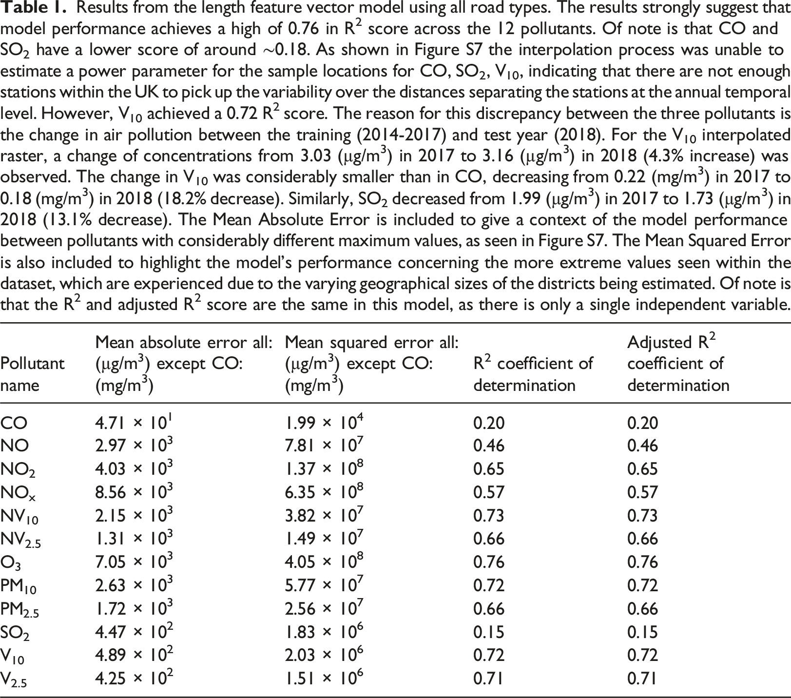
The R² score is the core metric that we use for comparing the accuracy of the models. We included the R² score in addition to the MAE and MSE because its upper bound of R² of 1 allows us to compare models that make predictions between target variables with large differences in magnitude. For example, as CO has a maximum value 10 orders of magnitude smaller than O₃, the MAE and MSE alone would not allow for comparison between a model that estimates CO and one that estimates O₃.

The R² score also embeds our baseline model for comparison (i.e., the null model for the problem), where a R² score of 0 represents a model that has predicted the mean for every time point in the series. Alongside the R² score, we also calculate the adjusted R² score. The adjusted R² score is defined in equation (1) as follows:

R_{adj}^{2} = 1 - \frac{(1 - R^{2}) (N - 1)}{N - p - 1},

(1)

where R² = coefficient of determination, 𝑝 = number of independent variables, and 𝑁 = total sample size.

The adjusted R² score measures the performance of each model while considering the number of independent variables, highlighting model improvements that occur by including additional variables over what would occur simply by chance and highlighting potential overfitting. Table 1 provides the results for the length model, but should be seen in conjunction to the other tables described later to allow a fair comparison between the models. An example feature vector for the length model can be seen in Table S2, with predictions made by the model shown in Table S5. Figure 1 depicts different subsets of the MSOA City of London 001 district road network structural properties. In relation to Figure 1 the model only considers the total length of the blue road network.

Figure 1.

Road network structure within MSOA City of London 001 (blue) and surrounding MSOAs (yellow). The solid black line represents the residential roads within MSOA City of London 001 and the dashed black line the residential roads within the neighbouring MSOAs. The road network will contribute differently to the feature vector values depending on the model used. In the case of the length model, the total length of the road network is used, which for MSOA City of London 001 is 223,092m, shown with the blue and black solid lines. In the composition model, each road type contributes to a different element in the feature vector, with the black solid residential roads contributing a single element of the feature vector with the value 23,235m. The spatial variant of the model considers the total road length for different road types in adjacent MSOAs alongside the considerations of the composition model, meaning the total for the dashed black line is a single element of the feature vector, which has a value of 82,500m.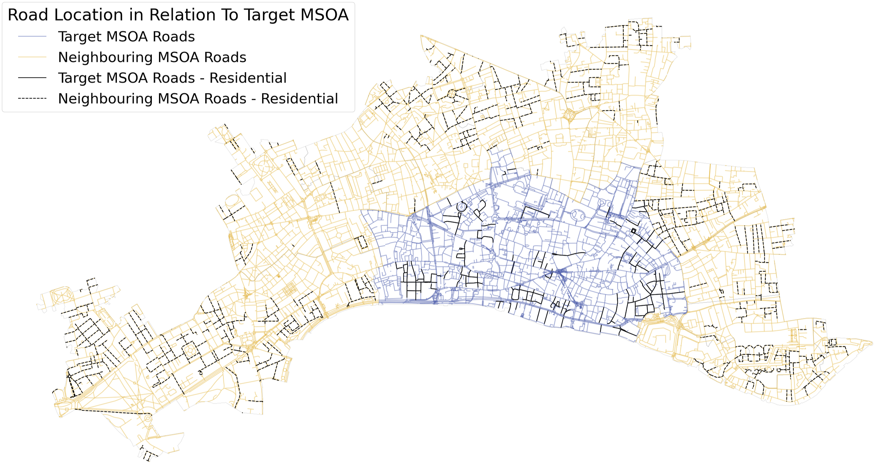

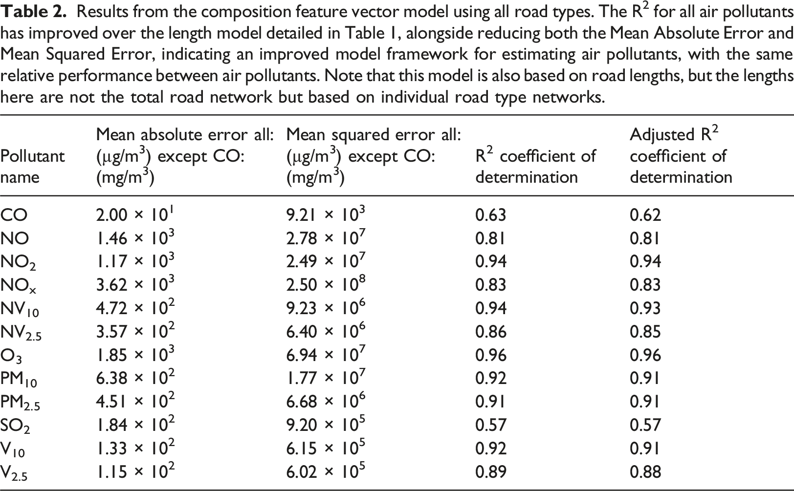
The second variation of the model splits the road network into the different road types as detailed in the OpenStreetMaps database (OpenStreetMap contributors, 2021), and creates a length element per road type in the feature vector. In relation to Figure 1 the feature vector still only considers the blue road network but now creates a separate feature for each road type, such as the solid black lines denoting the residential roads within the blue road network. An example feature vector for the composition model can be seen in Table S3, with predictions made by the model shown in Table S6. A decision tree regressor with multiple feature vector elements is used for this variation of the model. The results from this model can be seen in Table 2. These results show an average increase of 0.266 of the R² scores with respect to the scores obtained by the first model.

Table 2.

Results from the composition feature vector model using all road types. The R² for all air pollutants has improved over the length model detailed in Table 1, alongside reducing both the Mean Absolute Error and Mean Squared Error, indicating an improved model framework for estimating air pollutants, with the same relative performance between air pollutants. Note that this model is also based on road lengths, but the lengths here are not the total road network but based on individual road type networks.

Pollutant name	Mean absolute error all: (µg/m³) except CO: (mg/m³)	Mean squared error all: (µg/m³) except CO: (mg/m³)	R² coefficient of determination	Adjusted R² coefficient of determination
CO	2.00 × 10¹	9.21 × 10³	0.63	0.62
NO	1.46 × 10³	2.78 × 10⁷	0.81	0.81
NO₂	1.17 × 10³	2.49 × 10⁷	0.94	0.94
NO_x	3.62 × 10³	2.50 × 10⁸	0.83	0.83
NV₁₀	4.72 × 10²	9.23 × 10⁶	0.94	0.93
NV_2.5	3.57 × 10²	6.40 × 10⁶	0.86	0.85
O₃	1.85 × 10³	6.94 × 10⁷	0.96	0.96
PM₁₀	6.38 × 10²	1.77 × 10⁷	0.92	0.91
PM_2.5	4.51 × 10²	6.68 × 10⁶	0.91	0.91
SO₂	1.84 × 10²	9.20 × 10⁵	0.57	0.57
V₁₀	1.33 × 10²	6.15 × 10⁵	0.92	0.91
V_2.5	1.15 × 10²	6.02 × 10⁵	0.89	0.88

Our third model was a spatial variant of the second model, using the same decision tree framework as in the composition model. We created the spatial model to capture whether the district was in the centre of an urbanised zone, on the outskirts or wholly removed, as the primary sources of a district’s air pollution might be outside the district’s boundaries. The feature vector for the spatial model comprised the same features as the composition model; however, the process conducted for the blue road network within Figure 1 was repeated for the yellow road network, providing a total length of the adjacent district’s road networks, thereby doubling the number of features of the feature vector over the composition model, shown in Table S4. For two districts to be labelled as adjacent, they must share a border; if a water body (e.g., river) separates two districts, they are labelled as non-adjacent. Predictions made by the spatial model are shown in Table S7. By augmenting the feature vector of each district with the sum of road-network lengths by road type of the adjacent districts we provide the model with spatial context that allows the model to distinguish if a district is urban or rural. The results from this model are shown in Table 3.

Table 3.

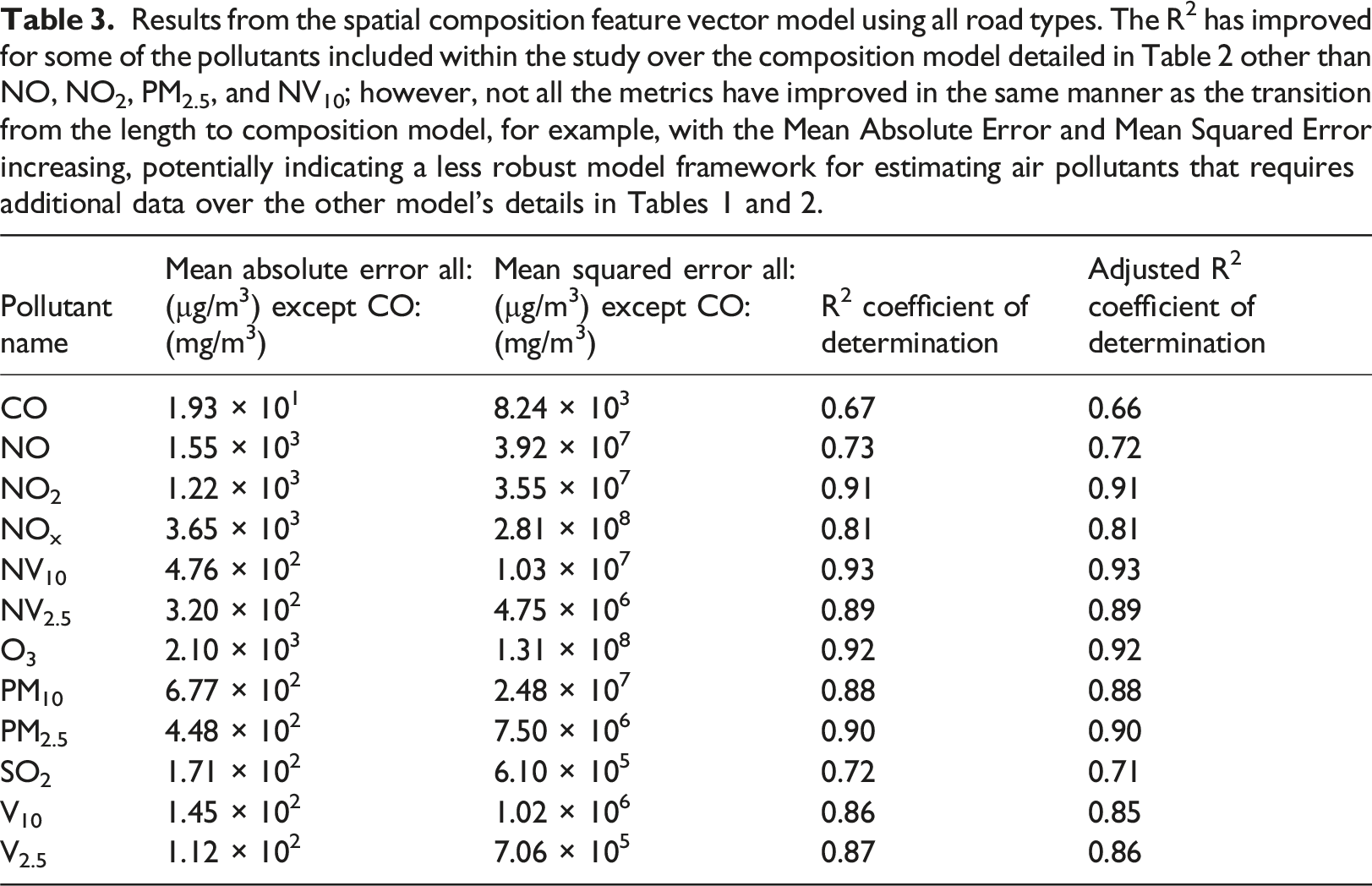
Results from the spatial composition feature vector model using all road types. The R² has improved for some of the pollutants included within the study over the composition model detailed in Table 2 other than NO, NO₂, PM_2.5, and NV₁₀; however, not all the metrics have improved in the same manner as the transition from the length to composition model, for example, with the Mean Absolute Error and Mean Squared Error increasing, potentially indicating a less robust model framework for estimating air pollutants that requires additional data over the other model’s details in Tables 1 and 2.

Pollutant name	Mean absolute error all: (µg/m³) except CO: (mg/m³)	Mean squared error all: (µg/m³) except CO: (mg/m³)	R² coefficient of determination	Adjusted R² coefficient of determination
CO	1.93 × 10¹	8.24 × 10³	0.67	0.66
NO	1.55 × 10³	3.92 × 10⁷	0.73	0.72
NO₂	1.22 × 10³	3.55 × 10⁷	0.91	0.91
NO_x	3.65 × 10³	2.81 × 10⁸	0.81	0.81
NV₁₀	4.76 × 10²	1.03 × 10⁷	0.93	0.93
NV_2.5	3.20 × 10²	4.75 × 10⁶	0.89	0.89
O₃	2.10 × 10³	1.31 × 10⁸	0.92	0.92
PM₁₀	6.77 × 10²	2.48 × 10⁷	0.88	0.88
PM_2.5	4.48 × 10²	7.50 × 10⁶	0.90	0.90
SO₂	1.71 × 10²	6.10 × 10⁵	0.72	0.71
V₁₀	1.45 × 10²	1.02 × 10⁶	0.86	0.85
V_2.5	1.12 × 10²	7.06 × 10⁵	0.87	0.86

Interestingly, the R² score only sometimes improves by adding more data from neighbouring districts. This is likely caused by the lack of available training data. As there are only 7201 districts within the study area and a total of 199 features are used, it is difficult to produce an optimal model. This lack of optimal model can be seen with the models that can all predict the air pollution to a similar degree of success (∼0.1 R² score) but isn’t consistently higher than the composition model. If the number of districts to be estimated were smaller and more numerous, such as the case of using the uniform grid approach discussed in Section S1 then the spatial variant of the model might show more promise and robustness.

Overall, the three different variations of the model provide a number of benefits. The length model is conceptually simple, allowing us to integrate multiple road network data sources, as the property of road length is uniform among datasets. The composition model improves the length model but restricts the datasets that can be used where the classification schema is consistent across the study period. Finally, the spatial model offers further performance improvements but requires much more data than the composition model, with some added model complexity.

Reducing the feature vector

The feature vector in the previously described models included all road types in the OpenStreetMaps dataset. There are 99 different road types, but some are misclassified (shown in tables in Section S3.3). This section describes how we reduced the dataset’s size to only what was needed for estimating air pollution within a district. Here, we relied on information theory (Shannon, 1948) and in particular mutual information between the road types and the different air pollutants to determine which road types have the highest relation with each air pollutant. First, the dataset was reduced to 88 road types by removing road types that had no relevance to the air pollutants being studied, represented by a mutual information summation value of 0. The types removed were mostly misclassifications by a user inputting a road type, such as “fence” or “residential;footway”. Next, we incrementally increased the threshold for removal for a road type summation value and compared the resulting model’s performance by its R² score. Figure 2(a) shows a plot of the resulting R² score for both the length and composition models against differing numbers of road types subset by the value of the threshold for inclusion of the mutual information summation. Table S8 shows mutual information values for the pollutants across a range of road types, and Table S9 shows the model’s performance with reduced input datasets.

Figure 2.

Model performance vs R² score, with road type inclusion based upon road type mutual information with air pollution. (a) Starting with all 99 road types. (b) Twenty five road types relevant to all air pollutants. Shown is the performance of the length and composition model when removing certain roads from being included as part of the feature vector. Inclusion in the feature vector depends on the sum of mutual information of the road type with pollutants considered in the study. A threshold is incremented to remove the road types with less mutual information than others. The requirement for a non-zero mutual information sum removes 11 road types with no relation to pollution, such as the OpenStreetMaps classification of turning circles, leaving 88 road types. Many road types have a minimal sum for mutual information, so incrementing the threshold to 0.1 removes 65 road types, with classifications such as living street removed. This process is then repeated until a single road type remains, in this case, the track road classification, which can be seen at which point the length and composition model reduces to the same model. Figure 2(b) details the same experiment detailed in Figure 2(a) however only road types that have a non-zero value for mutual information with all pollutants were considered, leaving 25 road types, removing road types such as lane that only have a non-zero mutual information values with SO₂.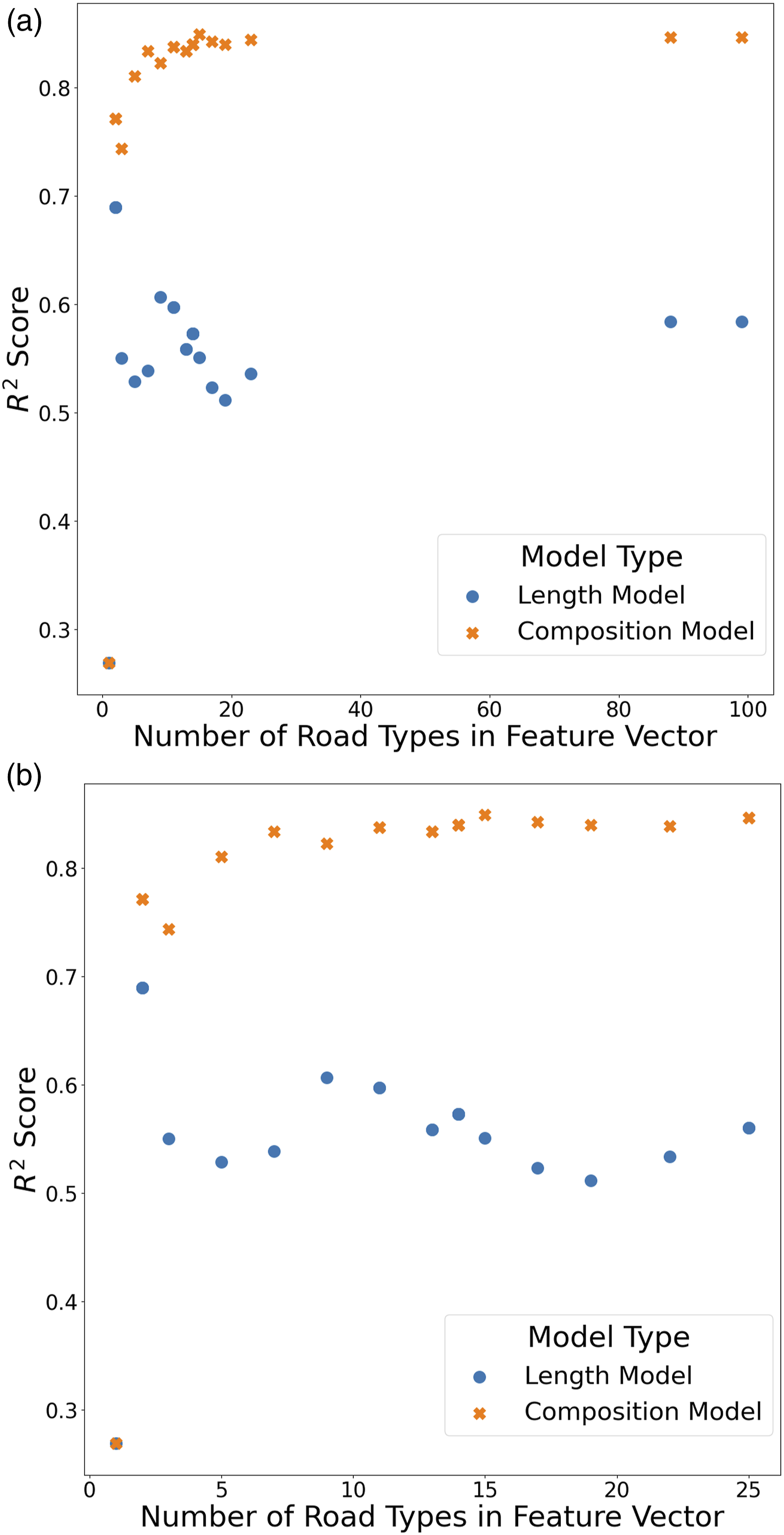

We then repeated the experiments; however, we included only road types relevant to all 12 pollutants in the test. Twenty five out of 99 road types had relevance to all 12 pollutants to be estimated; relevance is measured by ensuring that the road type had non-zero mutual information for all 12 pollutants. The results of this experiment are shown in Figure 2(b). Table S10 shows the results from the previous three models with road types with zero mutual information with at least one of the pollutants.

In Figure 2, the best length model uses two road types, track and unclassified, to predict the pollution within a district, seen distinctly with an increase in the R² score for the length model to 0.69, up from 0.27, with the composition model improving to 0.77 from 0.27 during the same test. We can see that some road types cause the length model to perform worse, but even when the result improves, it never performs as well as the composition model. Eventually, with only one road type remaining, the length and composition model are reduced to the same regression model, producing an R² score of 0.27. As shown in Figure 2, the length model is considerably more susceptible to variations in performance with changing input data than the composition model. However, the model can consistently predict the air pollution concentrations to similar performance, no matter the included road types.

Of note is the potentially confusing classification schema used in OpenStreetMaps. The classification of unclassified discussed is, in fact, a type of road. From the road type schema for OSM, advice to mappers is given “In other words, don’t use highway = unclassified just because you don’t know what road type it is. The value unclassified is indeed a classification, meaning ‘very minor road’.”⁷ The unclassified road type has been grandfathered in from the data within the UK and originally meant a road type small enough with different rules about signage.

We performed pairwise mutual information between the road types to further reduce the dataset. The goal was to determine the road network types that contained the most information about other road types within the dataset. The road types we performed the mutual information on were the 25 road types with some mutual information with every pollutant covered in the study. Figure 3 shows a heatmap of the mutual information values between the 25 road types. The values in the heatmap have been normalised row-wise. In the heatmap, there are 625 data points. 457 points have a value of mutual information greater than zero. Some data points have a value of 0 for mutual information; for example, living street and raceway have zero pairwise mutual information.

Figure 3.

Mutual information between road types. The heatmap shows the mutual information between all 25 road types, with a non-zero mutual information value with all the pollutants in the study. The heatmap values are normalised by row with the diagonal removed (which has value 1), allowing for an understanding of which road type has the highest mutual information to the other road types in the dataset. Motorway link has the highest mutual information with the motorway road type. While the motorway type has strong mutual information with the motorway link type, there are also strong mutual information scores with other road types, such as track and path. This difference in the strength of mutual information indicates that the motorway link dataset contains information mainly about the motorway road type, but the motorway dataset contains information about motorway link and other road types such as track, path etc., giving it a more desirable use in retaining information about all datasets (values are normalised by row and the diagonal removed).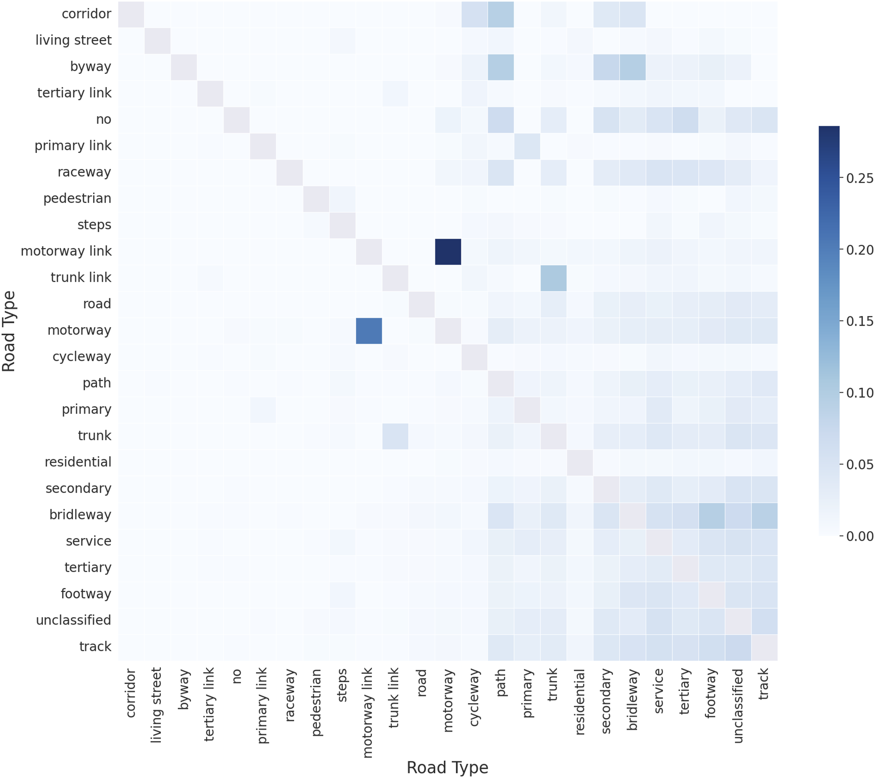

The heatmap was modelled as a network of the 25 road types to determine the road types that contain the most mutual information about other road types, as shown in Figure S11. Each node in the network represents a road type, and the edge weight between the two nodes is the mutual information between the two road types. The degree of each node is equal to the sum of the weights of the edges adjacent to the given node, giving a value for the amount of mutual information a given road type contains about other road types in the network.

The node with the highest degree was chosen for inclusion in the model feature vector and then removed from the network as the mutual information of the edges no longer needed to be included in the dataset. This process was repeated, with the next highest node based on degree weight chosen, until no nodes remained. The results of this process on the network representation can be seen in Figure S12.

The test results in Figure 4 show that a model underpinned by the “track” and “unclassified road” road types produces a model with an R² score of 0.69 for the length model and 0.77 for the composition model while only making use of 25.9% of the total road network length in the study area. Indicating that these two types of roads are sufficient to provide a good estimation of air pollution, and an improvement of 0.08 in performance is achieved when the distinction between road types is included in the model.

Figure 4.

Total inter road cumulative mutual information in input feature vector vs R² score. Shown is the performance of the length and composition model when removing road types from being included as part of the feature vector based on the road type’s mutual information with other roads, aiming to reduce the data required while maintaining performance by including road types containing information about other road types. A single road type was removed at each step, with the x-axis detailing the total remaining mutual information about other road types within the datasets used for the feature vector. Eventually, the model reduces into the same model when only a single road type remains. The performance improvement of the length model as some road types are removed indicates that some of the datasets included are noisy and affect model performance; this issue is not as prevalent with the composition model that can differentiate different road types, seen with a gradual reduction in model performance. The full experiment results can be seen in Table S11.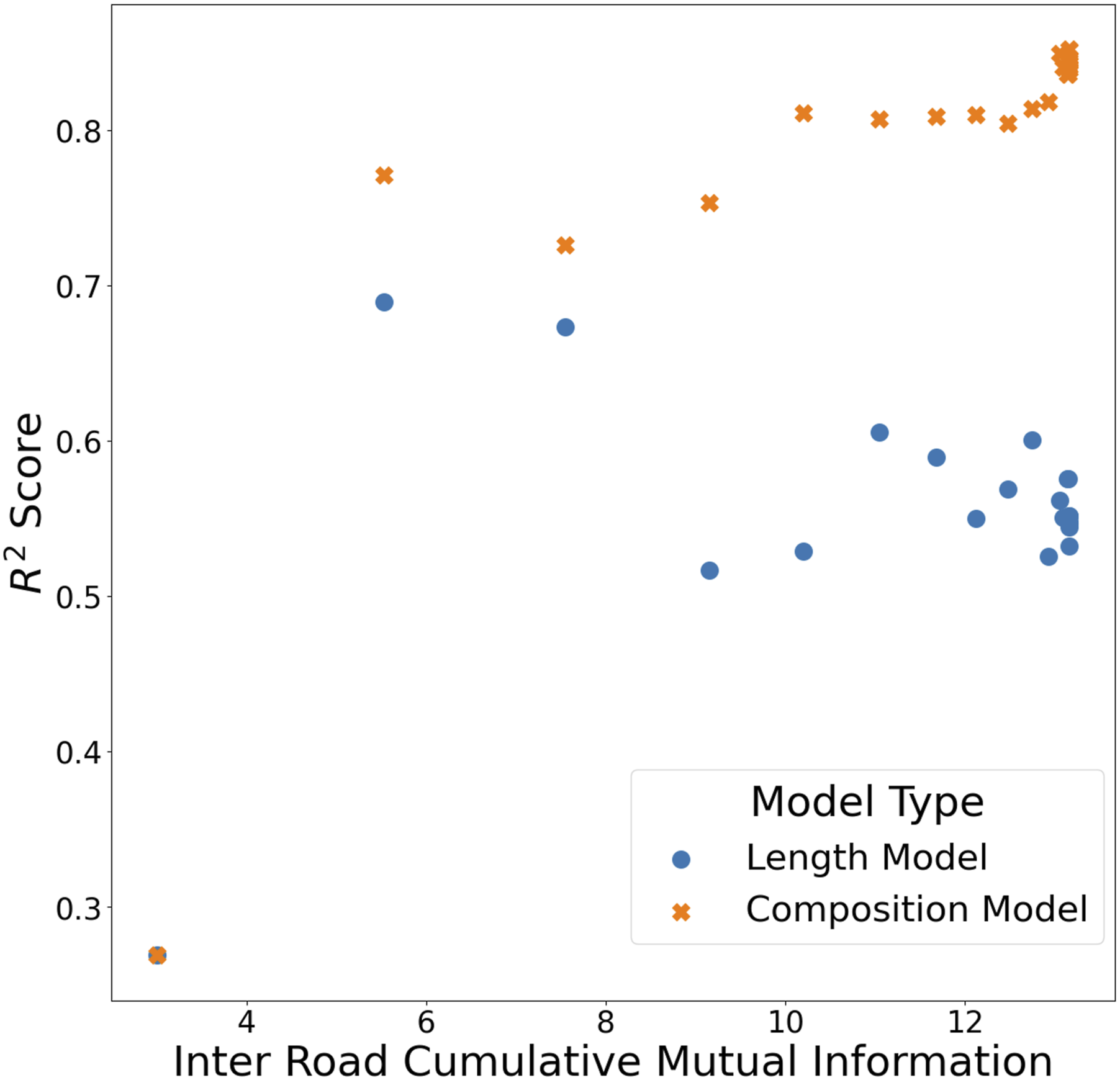

Quantity of missing districts

We conducted experiments to explore whether some districts within the study area could be used for training, having the remaining districts estimated from the model created. The goal is to understand the model’s performance in estimating all the district’s air pollution concentrations as the data available to train the model is reduced. We did not include the spatial variant in these tests, as it would require additional data acquisition over the minimal amount of measuring needed for just the district itself, e.g. if 100 districts were included in the training set, then road data would be needed for all adjacent districts to the 100 districts as well as the 100 districts themselves. We used the data from 2018 for the tests. For a set of 16 random choices, different MSOAs were randomly sampled from the 7201 total MSOA districts to create different size training and test sets, meaning that each of the test set sizes experiments was performed 16 times, with the spread of the performance depicted by the red shaded region in Figure 5. When selecting the additional districts to be included in the test, we ensured the districts used in the previous iterations were still present. For example, the districts used in one random state in the 100 training set size were also used in the 500 training set size, as visualised in Figure S13. Table S13 shows the results for the mean R² score for both the length and the composition model for reducing training set sizes across 16 random state tests. We explored test set sizes ranging from 100 MSOAs to 7200 MSOAs.

Figure 5.

Test set size districts vs R² score. The red-shaded region shows the range of performance of each model across the 16 random tests for a particular test set size, with the min and max at each set size bounding the region. (a) Length Model. (b) Composition Model. The performance of the length and composition model is shown as the input districts for the training set are reduced from 7101 to 1. As the test set size increases (and so the training set size decreases), the performance of both models remains stable until the test set comprises around 7100 data points (98.6%). At this point, the composition begins to break down with an apparent reduction in performance across some tests, indicated by the slope in the shaded region. The performance is then further reduced with subsequent smaller training set sizes. Across the experiments, the length model maintains a similar degree of performance compared to the composition model. Thereby indicating that while the composition model performs better than the length model initially, it does require more input data to perform well. The difference in the shaded region highlights the stability of the length model in comparison with the composition model when the training set size becomes small.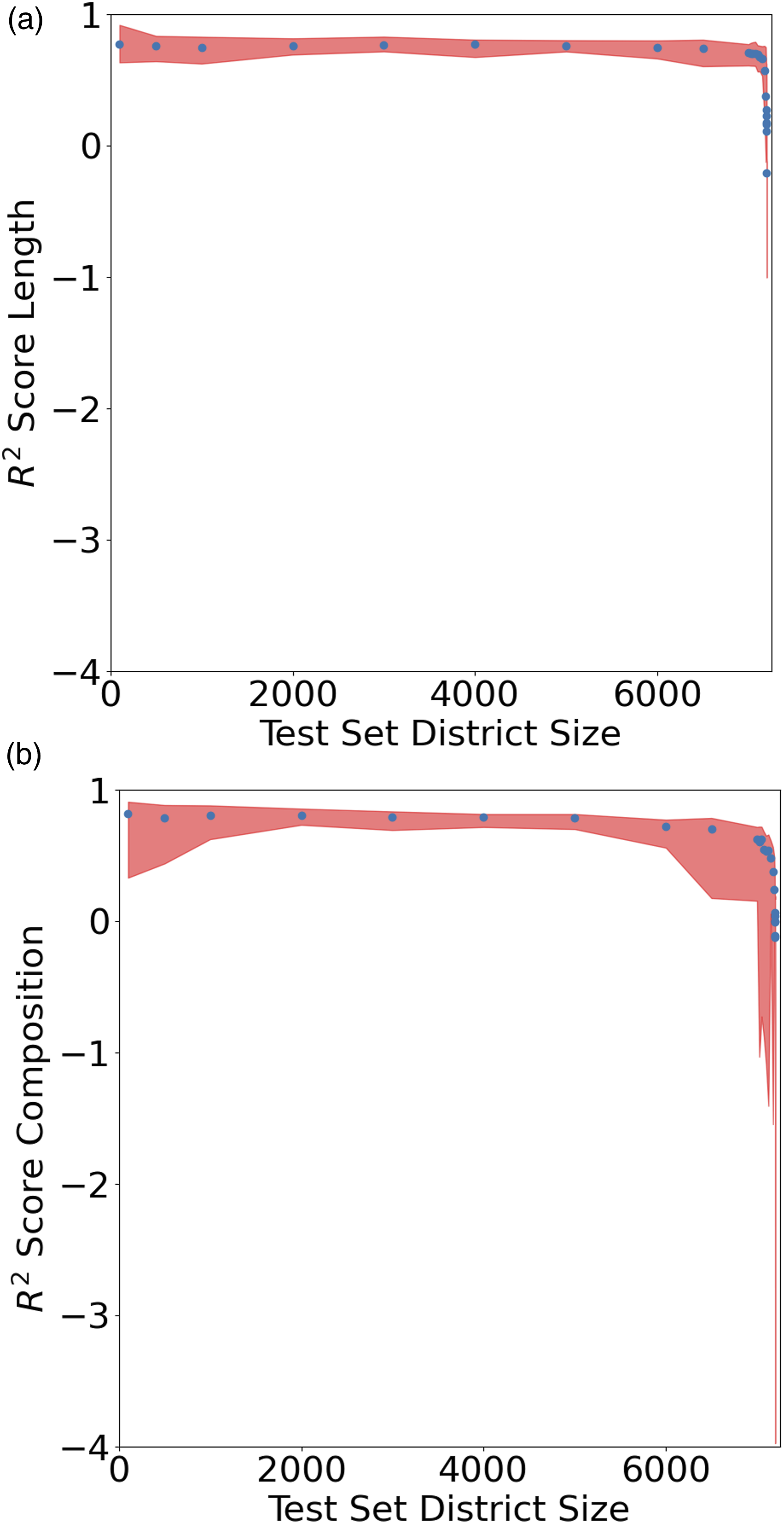

Figure 5 shows the scatter plots for the data detailed in Table S13, alongside providing a bound for the minimum and maximum values from the random tests performance via the red shaded region. The random tests show that the length model is more robust than the composition model, with the red-shaded region being considerably smaller, denoting a less variable performance across the 16 random tests for the length model. Thereby indicating that the composition of the road network between different districts can vary greatly, resulting in poor performance in some random training sets. The length model maintains performance as the training size is reduced from the initial 7101 MSOAs to 126 MSOAs, with an R² score of 0.6. After this, the performance of the model begins to decrease. Across a range of different random states, around 126 MSOAs must be used to train the model to successfully predict all MSOAs pollution, representing 1.75% of the total number of MSOAs. In the most extreme scenario seen in Figure S13 for one of the 16 random tests, training was performed on a single district, and the other 7200 districts in 2018 were estimated, which resulted in a catastrophic failure of the model with an R² score of less than 0 being achieved for both the Length and Composition model, representing a model that performs worse than simply estimating the mean air pollution concentrations across all districts. These experiments highlight that while the length model is more robust to changes in training data size, there is a limitation to both in regard to the data required, representing the core limitation of a data-driven supervised machine learning approach, where having enough data is crucial, with 126 districts emerging as the point in the context of England and Wales in 2018 as the minimum amount of data needed for consistent performance to be achieved in estimating all districts.

Urban and rural missing districts

A further experiment was conducted to examine how different types of districts affect model performance, particularly when trained on either predominately urban or rural districts, to ensure that the placement of monitoring stations does not affect performance. As highlighted in Figure S4 the distribution of the sensors is not uniform, and so a sampling error could be present. Population density was used as a proxy metric for how urbanised a district is, with higher population density districts being seen as more urban, with example districts shown in Table S12. As seen in Quantity of Missing Districts Figure 5 and Table S13, the R² score for the length model performed consistently with an R² of ∼0.7 as the training set size was reduced, providing the baseline for this experiment. We trained a set of models with 1500 districts with similar population densities to explore the effect of a changing population density distribution in the model’s training set on performance. The first data point starts with the least urbanised MSOAs, to the most urbanised MSOAs, with increments of 125. For each training set, a model was trained, and the R² score was computed. For example, the first experiment trained the model on the most urban 1500 districts and assessed the model performance on the other 5701 districts. The results from this experiment are shown in Figure 6, where the average R² score across the 46 tests was an R² score of 0.83. The R² score remained similar to the expected ∼0.8 from the reducing training set sizes experiment detailed in Quantity of Missing Districts as the training set changed from least to most urbanised. Thus, pointing toward the idea that the R² score of the length model is not related to the population density distribution of the MSOAs included in the subset of training districts.

Figure 6.

Test sizes vs R² score for length model for changing population density within the training set. Shown is the length model’s performance across a range of training sets chosen based on the MSOAs population density. The population density for an MSOA is used as a proxy for how urbanised an MSOA is; the higher the population density, the more urbanised an MSOA is. 1500 MSOAs were chosen to be part of each training set, with the variation being in the average population density of the training set MSOAs. The first point (Min 0 Max 1499) is where the least urbanised MSOAs are the training set. The last point (Min 5625 Max 7124) is where the most urbanised MSOAs are the training set. The consistent performance of the length model as the average urbanisation of the training set MSOAs increases indicates how urbanised an MSOA does not affect the model performance. Table S14 shows the full experiment results.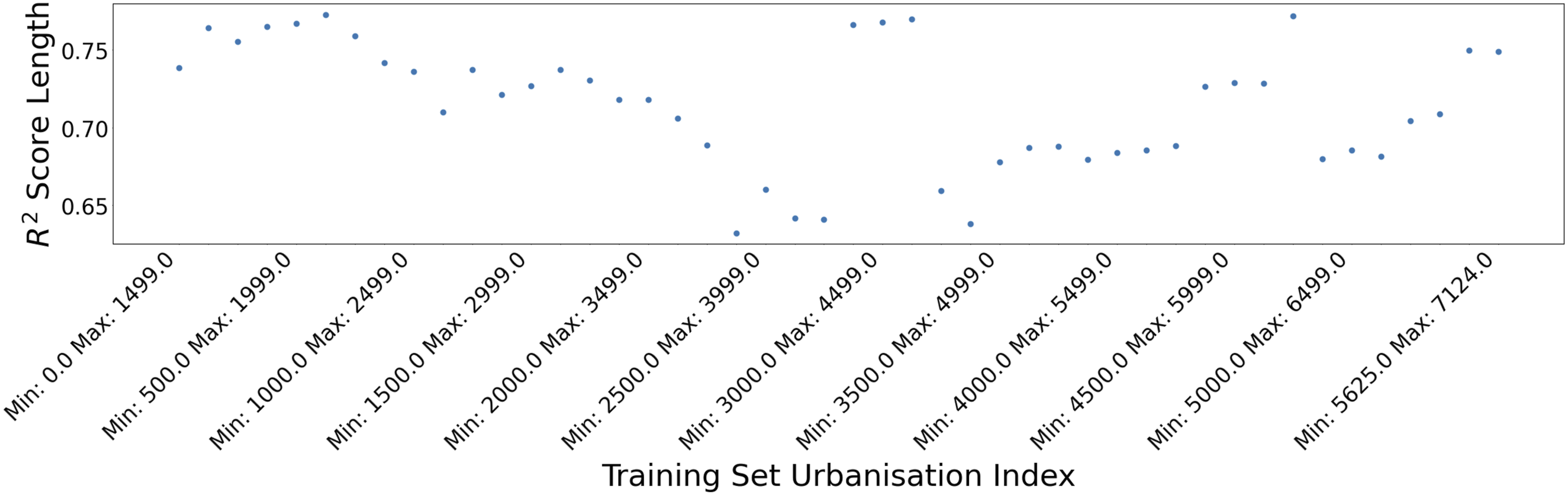

Inter country missing districts

The final experiment we conducted explored the possibility of estimating one country’s air pollution concentrations by training the model on another country. Two experiments were conducted, estimating Welsh air pollution concentrations from a model trained on England, the results of which can be seen in Table 4 and the reverse experiment seen in Table 5. The model’s performance when estimating Wales from being trained in England is ∼0.8 across all pollutants, with a performance of ∼0.63 for estimating England from Wales. The difference in performance can be explained by the difference in the amount of training data, namely that within Wales, there are only 462 districts for training, and 6739 districts in England, visualised in Figure S14. These results align with the experiment in Quantity of Missing Districts and further support the importance of the amount of data required for the adequate performance of a data-driven supervised machine learning model. Of note is that while these countries are incredibly similar, they do provide an initial first signal for the experiment to be expanded to be more diverse countries in future work.

Table 4.

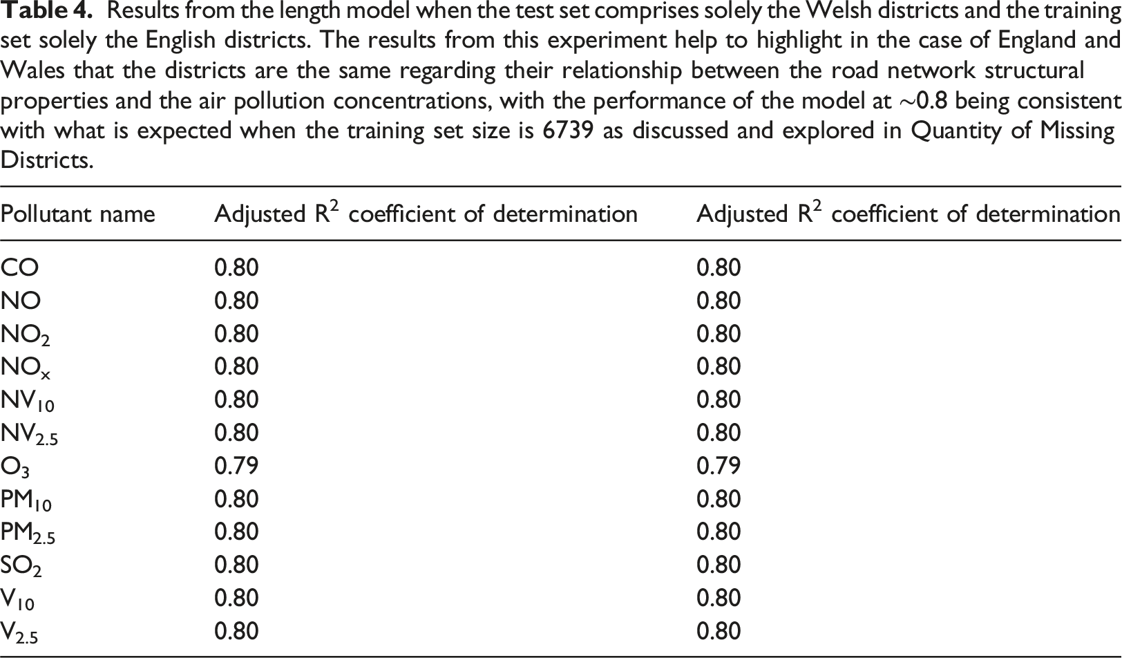
Results from the length model when the test set comprises solely the Welsh districts and the training set solely the English districts. The results from this experiment help to highlight in the case of England and Wales that the districts are the same regarding their relationship between the road network structural properties and the air pollution concentrations, with the performance of the model at ∼0.8 being consistent with what is expected when the training set size is 6739 as discussed and explored in Quantity of Missing Districts.

Pollutant name	Adjusted R² coefficient of determination	Adjusted R² coefficient of determination
CO	0.80	0.80
NO	0.80	0.80
NO₂	0.80	0.80
NO_x	0.80	0.80
NV₁₀	0.80	0.80
NV_2.5	0.80	0.80
O₃	0.79	0.79
PM₁₀	0.80	0.80
PM_2.5	0.80	0.80
SO₂	0.80	0.80
V₁₀	0.80	0.80
V_2.5	0.80	0.80

Table 5.

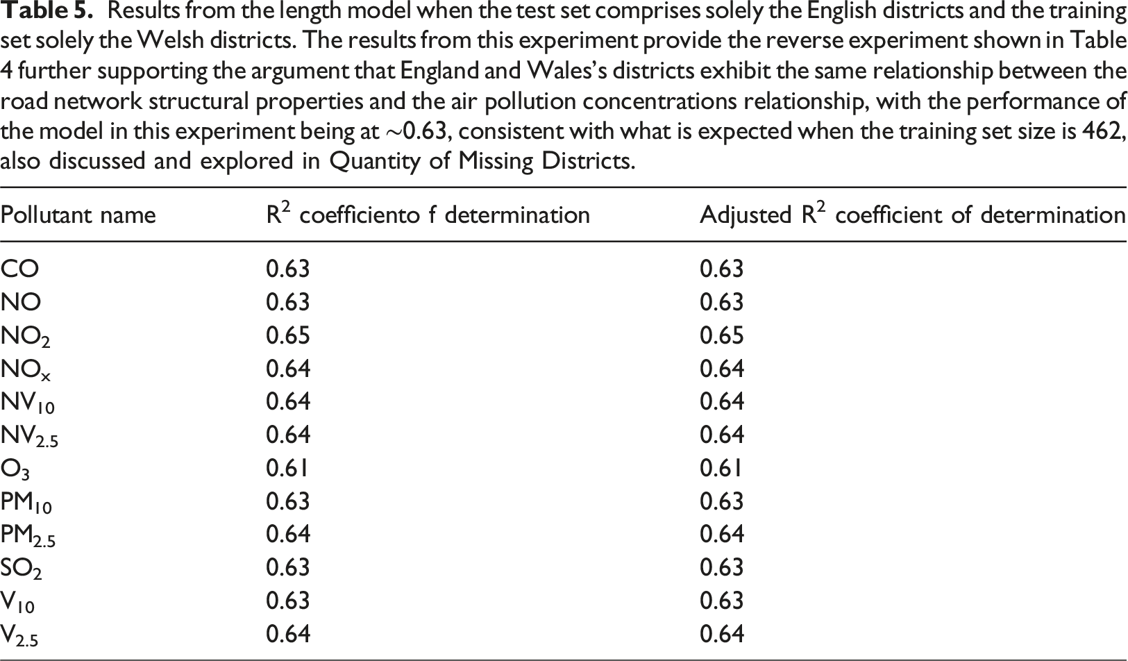
Results from the length model when the test set comprises solely the English districts and the training set solely the Welsh districts. The results from this experiment provide the reverse experiment shown in Table 4 further supporting the argument that England and Wales’s districts exhibit the same relationship between the road network structural properties and the air pollution concentrations relationship, with the performance of the model in this experiment being at ∼0.63, consistent with what is expected when the training set size is 462, also discussed and explored in Quantity of Missing Districts.

Pollutant name	R² coefficiento f determination	Adjusted R² coefficient of determination
CO	0.63	0.63
NO	0.63	0.63
NO₂	0.65	0.65
NO_x	0.64	0.64
NV₁₀	0.64	0.64
NV_2.5	0.64	0.64
O₃	0.61	0.61
PM₁₀	0.63	0.63
PM_2.5	0.64	0.64
SO₂	0.63	0.63
V₁₀	0.63	0.63
V_2.5	0.64	0.64

Use cases

We contend that the crucial road types to predict the air pollution in an area are the minor roads; the road types “track” and “unclassified” within the OpenStreetMaps classification schema. These road types not only exhibit the highest mutual information regarding the 12 pollutants analyzed in this study, with normalised summation values of 12 and 10.12, respectively, but they also display the most mutual information concerning the other road types, with total values of 2.97 and 3.00, respectively. The “track” and “unclassified” road type input data produce a model with an R² score of 0.69 for the length model and 0.77 for the composition model. The model then degrades to an R² score of 0.27 when only the “track” road type is included, where the length and composition model is the same. The R² score of the complete composition model (i.e., all 25 road types), improves to 0.85 compared to the length model’s R² score of 0.58. An argument is that the increased amount of data (an additional 23 road types) needed to attain the increase of 0.08 on the R² for the composition model is not worthwhile. The entire length of the road network within the MSOA boundaries in 2018 is 1,140,835,548 m, out of which 295,948,514 m, represents the “track” and “unclassified” road network, representing a 74.1% reduction in input data for minimal performance loss in the case of the composition model. However, it is also vital to consider the context in which the model is intended for use. The primary purpose of the model was never to provide precise predictions of air pollution levels to specific values, but rather to offer insights into the areas with the highest pollution within a given region, aiding in the identification of suitable areas for intervention. From this perspective, the loss of 0.08 R² score holds little significance in the model’s practical application.

The implications of the missing district tests are significant for deploying monitoring stations to create a target vector. The experiment, as detailed in Quantity of Missing Districts, examined the number of districts needed to generate a complete air pollution concentration map for England and Wales in 2018. The results strongly suggested that a mere 1.75% of districts, amounting to 126 out of 7201 districts, were sufficient to predict air pollution concentrations across all districts at the annual level. Furthermore, the experiments presented in Urban and Rural Missing Districts indicated that considering the distribution of urban, suburban, and rural districts in the training set is unnecessary. Using the proposed model would allow policymakers to have full spatial coverage of air pollution while only deploying monitoring stations in 1.75% of districts, representing significant monetary savings over deploying a comprehensive air pollution monitoring network like the UK’s AURN. While acknowledging their similarity, there is also a positive first signal that the model can move between countries, as was the case between England and Wales in 2018 as explored in Inter Country Missing Districts.

The findings of this study show that a decision tree regression model underpinned by a single structural property, length, of the road network within 1.75% of districts within England and Wales in 2018 was enough data to identify an ordering of which districts are the most polluted. Furthermore, the model discussed presents a low-cost method of achieving similar results to more expensive models such as MAAQ currently used by DEFRA. The model exhibits evident practical utility for policymakers aiming to pursue clean air initiatives while facing budget constraints that hinder investments in comprehensive dedicated monitoring networks across vast spatial areas. By offering a viable first step, it helps mitigate the inequality in air pollution information between countries equipped with sophisticated air pollution models and robust, extensive monitoring station networks and those that lack such resources.

Limitations and transferability

While the model presented works towards a generalisable model for estimating air pollution concentrations from road networks that can move between countries, there are limitations associated with the model that impact its application in particular scenarios. The key point regarding the model’s usability is ensuring that the data available for air pollution concentrations and the road network is of sufficient quantity and quality to underpin the model. As the model used is data-driven, there is a need for some data. An explicit limitation is a requirement for a country to possess some data concerning road and air pollution, with the particular quantity being different for each country, depending on the country’s diversity concerning air pollution. However, suppose a country does not currently have the required data. In that case, this work provides a blueprint for what they can work towards regarding data quality and the minimal data requirements. This work outlines England and Wales, with future work aiming to confirm minimum data requirements for other countries.

There are two possible issues with moving a model trained in the UK to another. The first is ensuring that all the roads within a country (or area of interest) have been mapped, and the second is ensuring that the road classification system is consistent if using the composition or spatial composition model. While OpenStreetMap (OSM) has global coverage, a road may have yet to be mapped due to the citizen science approach used. For the UK, the OSM road network is known to be complete. The proportion of roads mapped within the UK by OSM has recently been confirmed in a study by Microsoft. The study mined road networks globally,⁸ showing that for the UK (and Europe), the OpenStreetMap dataset was complete. However, the study revealed that the road networks in OSM are incomplete in certain countries. In addition to validating the completeness of the OSM database across various regions, the study made the Microsoft Missing Roads Study Dataset open-source, providing a comprehensive road network dataset covering the entire globe. The Microsoft Missing Road Study Dataset provides a dataset that addresses the second challenge in using our approach: an inconsistent road classification schema within OpenStreetMap.

The Microsoft dataset introduces a unified classification scheme for all road types from a single authoritative source, eliminating inconsistencies observed in OSM where road classification might vary by region. This standardisation ensures that the functional definition of a secondary road in England and Wales aligns with that in another country, facilitating the transferability of the model across diverse regions.

Another noteworthy limitation of the proposed approach lies in its vulnerability to system shocks, exemplified by events like the COVID-19 pandemic. While road networks contribute to air pollution, it is the traffic traversing these roads that serves as the primary source. In the model presented in this paper, data related to the road network serves as a cheap-to-collect proxy for various phenomena, including traffic, which influences air pollution concentrations.

It is crucial to recognise that the model is most effective in scenarios devoid of systemic shocks. In the event of such shocks, like the unprecedented changes observed during the COVID-19 pandemic, the model may lose accuracy. Addressing this limitation requires retraining the model with data reflecting the new state of the system. In such circumstances, it is essential for policymakers to exercise caution and assess the model’s appropriateness, considering the impact of the system shock on its performance.

Nevertheless, an alternative strategy exists to enhance the model by incorporating data related to system shocks, such as real-time traffic flows. This augmentation could enable the model to discern changes in air pollution concentrations linked to variations in traffic, thus mitigating the need for frequent model retraining. It’s worth noting that this approach comes with associated costs, involving coarse-level data wrangling and potential privacy concerns, especially for high-resolution data (Herrera et al., 2010). Therefore, there are distinct advantages to maintaining a model grounded solely in the structural properties of road networks. Its simplicity and ease of implementation make it adaptable to various scenarios, highlighting its utility even in the absence of real-time, fine-grained data.

Discussion

In this work, we have presented a solution for estimating annual air pollution using a dataset related to the structure of roads. Our primary focus lies on a model based on the length of roads, alongside a composition model that considers other factors associated with road classifications.

Our contributions can be split into three categories. (1) We have demonstrated the ability to achieve robust annual estimations on a significantly low budget, a marked contrast to the current costly approaches employed in the UK, amounting to millions of pounds. This cost-effective and accessible approach fosters inclusivity, enabling multiple stakeholders to utilise the estimations for various secondary applications, such as health exposure, traffic analysis, and city planning. (2) Our model’s interpretability extends even to a layperson, owing to its utilisation of easily explainable characteristics and simple regression-based estimators. This emphasis on transparency enhances the approach’s reusability and generality. (3) This work holds broader significance by showcasing how data science, particularly in the realm of environmental data, can effectively overcome data scarcity related to specific phenomena like air pollution. By harnessing information embedded in alternative datasets, even if not originally collected for this purpose, we achieve substantial progress. The concept of mutual information underpins this approach, wherein insights from one phenomenon can be gleaned from seemingly unrelated pieces of information, thereby providing valuable insights despite the constraints of limited data availability.

The presented approach presents numerous advantages, including a cost-effective implementation owing to the open-source nature of the data, minimal training computation, and an accessible model design. The experiments involving missing districts provide a framework for employing a limited number of monitoring stations across an area, such as 1.75% of MSOAs in the case of the UK, and utilise the presented model to estimate air pollution levels in the missing districts, thus generating a comprehensive spatial map of annual air pollution. This spatial map ensures that all districts, irrespective of their urban, suburban, or rural nature, receive estimates for ambient air pollution. This approach is especially valuable as it helps address inequality associated with the current focus on urban areas with monitoring station placement.

The UK and numerous other countries in the HIC and HMIC categories have the means to invest in comprehensive monitoring-station networks. However, the same opportunity may not always extend to countries classified as LIC or LMIC, particularly in many regions of the global south. The availability of global data concerning annual air pollution would significantly assist policymakers in making informed decisions and combating the alarming 4.2 million deaths per year attributed to ambient air pollution (Public Health, Social and Environmental Determinants of Health Department, 2018). Furthermore, when combined with the global accessibility of road structural properties’ data, the framework presented in this study serves as a foundation for future endeavours aimed at designing a global annual air pollution model using analogous secondary datasets. Such an approach holds promise for expanding our understanding of air pollution dynamics on a global scale.

Although the model presented does not directly incorporate specific polluting entities like point source emitters, it demonstrates remarkable accuracy in predicting annual air pollution levels. Our argument centres around the fact that any key polluting emitter must have accompanying supporting infrastructure, typically in the form of a road network, that the model can identify and utilise for estimations. Consequently, while it may not explore counterfactual scenarios involving the placement of point source emitters, once the supporting road infrastructure is comprehended, the model can make reliable predictions. This is a crucial point for us because the road structure itself contains valuable information about such emitters. For instance, if a factory is established in a particular location, it will inevitably depend on the road infrastructure for accessibility. Hence, the existing road structure often suffices for us to conduct annual estimations of air pollution, even without direct consideration of individual point source emitters.

The performance of low-cost air quality sensors is rapidly improving (Karagulian et al., 2019). While these improvements make it possible for LMIC to build cheaper monitoring networks, they provide data moving forward. Our model can potentially be used with the low-cost sensors to provide historical air-pollution estimations based on available historical road network data, either from OpenStreetMaps or recent advancements such as the Microsoft dataset, helping to build up a picture of how air pollution has changed over a considerable temporal period, alongside providing a stop-gap until the complete low-cost sensor monitoring network is operational.

In future work, we aim to extend the application of the same framework to estimate air pollution at a higher temporal resolution, such as the daily or hourly level. However, it is essential to acknowledge that there might be limitations to the approach presented in this paper when dealing with a finer temporal scale. The static nature of road transport infrastructure, combined with the influence of other environmental variables, could impact its effectiveness. Subsequent research will highlight the need to transition from data concerning the static elements of the road, such as its length, to more dynamic aspects of the road, such as the traffic counts of different types of vehicles. However, this data is more expensive to acquire and more invasive to privacy. Therefore, critical evaluations are needed whether the benefits derived from the model underpinned by more invasive dynamic data are worth the additional benefits of more accurate air pollution environmental intelligence.

Supplemental Material

Supplemental Material - Estimating annual ambient air pollution using structural properties of road networks

Supplemental Material for Estimating annual ambient air pollution using structural properties of road networks by Liam Berrisford, Eraldo Ribeiro, and Ronaldo Menezes in Environment and Planning B: Urban Analytics and City Science

Footnotes

Declaration of conflicting interests

The author(s) declared no potential conflicts of interest with respect to the research, authorship, and/or publication of this article.

Funding

The author(s) disclosed receipt of the following financial support for the research, authorship, and/or publication of this article: This work was supported by the Engineering and Physical Sciences Research Council and Liam Berrisford is supported by a UKRI Studentship at the Centre for Doctoral Training for Environmental Intelligence at the University of Exeter.

Data Availability Statement

The data that support the findings of this study are available on request from the corresponding author.

Supplemental Material

Supplemental material for this article is available online.

Notes

Liam Berrisford is a Postgraduate Researcher at the UKRI Environmental Intelligence Centre for Doctoral Training at the University of Exeter. With a Computer Science and Software Engineering background, his research focuses on tackling environmental challenges using machine learning.

Eraldo Ribeiro is an Associate Professor of Computer Sciences at Florida Institute of Technology. In 2001, he was awarded a Ph.D. degree in Computer Vision in the Department of Computer Science at the University of York, U.K. My research interests are in the areas of Computer Vision and Pattern Recognition, with a focus on the analysis of spatiotemporal patterns in images, videos, and acoustic signals. Most recently, I have been also working on the mathematical analysis and modeling of spatiotemporal patterns from social-media data.

Ronaldo Menezes is a Professor of Data and Network Science, and Director of the BioComplex Laboratory. His research interests include Network Science, Human Dynamics and Mobility, Complex Systems, and Urban Systems. He’s deeply involved with the research community in Human Mobility and Network Science and is currently the editor-in-chief of one of the main journals in the field: Applied Network Science published by Springer Nature.

References

Agrawal

(2005) Effects of air pollution on agriculture: an issue of national concern. National Academy Science Letters 28(3/4): 93–106.

Aunan

Hansen

Liu

, et al. (2019) The hidden hazard of household air pollution in rural China. Environmental Science & Policy 93: 27–33.

Breiman

(2017) Classification and Regression Trees. Abingdon-on-Thames, England: Routledge.

Brookes

Stedman

Kent

, et al. (2021). Technical Report on UK Supplementary Assessment under the Air Quality Directive (2008/50/EC), the Air Quality Framework Directive (96/62/EC) and Fourth Daughter Directive (2004/107/EC) for 2017. Technical report, Ricardo Energy and Enviroment. https://ukair.defra.gov.uk/assets/documents/reports/cat09/2102111100_2019_PCM_technical_report.pdf.

Brown

Barnes

Hayes

(2021) Traffic-related air pollution reduction at UK schools during the Covid-19 lockdown. Science of The Total Environment 780: 146651.

Carslaw

Ropkins

(2012) openair — An R package for air quality data analysis. Environmental Modelling & Software 27–28(0): 52–61.

Catalano

Galatioto

Bell

, et al. (2016) Improving the prediction of air pollution peak episodes generated by urban transport networks. Environmental Science & Policy 60: 69–83.

Daintith

(2009) A dictionary of physics. Root Mean Square Value (RMS Value). 6 ed. Oxford, England: Oxford University Press.

DEFRA Network eTendering Portal . (2021) Modelling of Ambient Air Quality Contract. Technical report. Department for Environment, Food and Rural Affairs. https://www.find-tender.service.gov.uk/Notice/007858-2021?origin=SearchResults&p=1. [Online; accessed August-2021].

10.

Deng

Mendelsohn

(2021) The effect of urbanization on air pollution damage. Journal of the Association of Environmental and Resource Economists 8(5): 955–973.

11.

Department of Environment, Food and Rural Affairs . (2019a) Air Pollution in the UK 2019 - Chapter 3 the Evidence Base. Technical report. UK Government.

12.

Department of Environment, Food and Rural Affairs . (2019b) Modelled Background Pollution Data PM25. https://uk-air.defra.gov.uk/data/pcm-data [Online; accessed August- 2021].

13.

Draper

Smith

(1998) Applied Regression Analysis. New Jersey, USA: John Wiley and Sons, volume 326.

14.

Chen

, et al. (2018) Household air pollution and personal exposure to air pollutants in rural China–a review. Environmental Pollution 237: 625–638.

15.

Eustice

of Richmond Park

(2021) Environment Bill. https://bills.parliament.uk/bills/2593 [Online; accessed August-2021].

16.

Gualtieri

Tartaglia

(1998) Predicting urban traffic air pollution: a GIS framework. Transportation Research Part D: Transport and Environment 3(5): 329–336.

17.

Henze

Hakami

Seinfeld

(2007) Development of the adjoint of geos-chem. Atmospheric Chemistry and Physics 7(9): 2413–2433.

18.

Herrera

Work

Herring

, et al. (2010) Evaluation of traffic data obtained via gps-enabled mobile phones: the mobile century field experiment. Transportation Research Part C: Emerging Technologies 18(4): 568–583.

19.

Hoek

Beelen

De Hoogh

, et al. (2008) A review of land-use regression models to assess spatial variation of outdoor air pollution. Atmospheric Environment 42(33): 7561–7578.

20.

Jacobson

(2008) On the causal link between carbon dioxide and air pollution mortality. Geophysical Research Letters 35(3).

21.

Johnson

(2017) Holding polluting countries to account for climate change: is “loss and damage” up to the task? The Review of Policy Research 34(1): 50–67.

22.

Karagulian

Barbiere

Kotsev

, et al. (2019) Review of the performance of low-cost sensors for air quality monitoring. Atmosphere 10(9): 506.

23.

Karlsson

(2002) The North-South knowledge divide: consequences for global environmental governance. Global Environmental Governance: Options and Opportunities, 1–24.

24.

Karppinen

Kukkonen

Elolähde

, et al. (2000) A modelling system for predicting urban air pollution: model description and applications in the helsinki metropolitan area. Atmospheric Environment 34(22): 3723–3733.

25.

Kelly

Fussell

(2015) Air pollution and public health: emerging hazards and improved understanding of risk. Environmental Geochemistry and Health 37(4): 631–649.

26.

Landrigan

(2017) Air pollution and health. The Lancet Public Health 2(1): e4–e5.

27.

Liu

Yan

Duan

, et al. (2021) Intelligent modeling strategies for forecasting air quality time series: a review. Applied Soft Computing 102: 106957.

28.

Mannucci

Franchini

(2017) Health effects of ambient air pollution in developing countries. International Journal of Environmental Research and Public Health 14(9): 1048.

29.

OpenStreetMap contributors (2021a) Key:highway OpenStreetMap Wiki.

30.

OpenStreetMap contributors (2021b) OpenStreetMap. https://www.openstreetmap.org [Online; accessed August-2021].

31.

Pak

Ryu

, et al. (2020) Deep learning-based pm2. 5 prediction considering the spatiotemporal correlations: a case study of Beijing, China. The Science of the Total Environment 699: 133561.

32.

Pellow

(2000) Environmental inequality formation: toward a theory of environmental injustice. American Behavioral Scientist 43(4): 581–601.

33.

Public Health, Social and Environmental Determinants of Health Department (2018) Burden of disease from ambient air pollution for 2016. Technical report. Geneva, Switzerland: World Health Organisation. World Health Organiization 1211 geneva 27 Switzerland.

34.

Qing

(2018) Urbanization and global health: the role of air pollution. Iranian Journal of Public Health 47(11): 1644–1652.

35.

Santana

Botta

Barbosa

, et al. (2023) Covid-19 is linked to changes in the time–space dimension of human mobility. Nature Human Behaviour 7: 1729–1739.

36.

Scoggins

Kjellstrom

Fisher

, et al. (2004) Spatial analysis of annual air pollution exposure and mortality. The Science of the Total Environment 321(1-3): 71–85.

37.

Shaddick

Thomas

Mudu

, et al. (2020) Half the world’s population are exposed to increasing air pollution. NPJ Climate and Atmospheric Science 3(1): 23.

38.

Shannon

(1948) A mathematical theory of communication. Bell System Technical Journal 27(3): 379–423.

39.

Shepard

(1968) A two-dimensional interpolation function for irregularly-spaced data Proceedings of the 1968 23rd ACM National Conference, August 27–29,1968, New York, NY, USA, 517–524.

40.

Stern

Builtjes

Schaap

, et al. (2008) A model inter-comparison study focussing on episodes with elevated pm10 concentrations. Atmospheric Environment 42(19): 4567–4588.

41.

Stevenson

Yardley

Stacey

, et al. (2009) QA QC Procedures for the UK Automatic Urban and Rural Air Quality Monitoring Network (AURN). Technical report. London, England: Department of Environment, Food and Rural Affairs.

42.

Stewart-Evans

(2019) Review of Interventions to Improve Outdoor Air Quality and Public Health. Technical report. Public Health England, Public Health England Wellington House 133-155 Waterloo Road London SE1 8UG https://www.gov.uk/government/publications/improving-outdoor-air-quality-and-health-review-of-interventions ([Online; accessed September-2022].

43.

Talbi

Kerchich

Kerbachi

, et al. (2018) Assessment of annual air pollution levels with pm1, pm2. 5, pm10 and associated heavy metals in Algiers, Algeria. Environmental Pollution 232: 252–263.

44.

Yan

Liao

Yang

, et al. (2021) Multi-hour and multi-site air quality index forecasting in Beijing using cnn, lstm, cnn-lstm, and spatiotemporal clustering. Expert Systems with Applications 169: 114513.

Supplementary Material

Please find the following supplemental material available below.

For Open Access articles published under a Creative Commons License, all supplemental material carries the same license as the article it is associated with.

For non-Open Access articles published, all supplemental material carries a non-exclusive license, and permission requests for re-use of supplemental material or any part of supplemental material shall be sent directly to the copyright owner as specified in the copyright notice associated with the article.

0.00 MB

10.81 MB