Sage Journals: Discover world-class research

Abstract

Energy-efficient urban development and carbon footprints (CFs) are often discussed in relation to climate change. The optimal level of urban density from a carbon reduction perspective at the city level has been much debated. However, considering possible trade-offs or co-benefits for CFs in the housing and travel sectors, it remains difficult to evaluate how intra-urban/residential densities and mixed land-use patterns relate to individual CFs at a community level in different seasons. The study objective was to demonstrate the changes in the CFs of residents in summer and winter according to spatiotemporal changes in urban forms, such as intra-urban/residential densities and mixed land-use patterns. Based on geographical data and CF survey results from Seoul and Gyeonggi in 2009 and 2018, four path analysis models were used to verify the spatiotemporal variances of the relationships between urban forms and the CFs of the housing/travel sectors (HCF/TCF). Path analysis with a set of mediation variables enables the evaluation of possible trade-offs, or co-benefits, when investigating the impacts of different measures of intra-urban densities and mixed land-use patterns on the CFs. Furthermore, the moderating effects of different cooling and heating patterns in different seasons on CFs were verified by comparing the four path analysis models in different spatiotemporal contexts. The results showed spatiotemporal changes in urban density and different impacts of urban and residential densities on the TCF. It was also revealed that a low percentage of residential land use in urbanized areas offsets the advantage of high density in reducing TCF and HCF. Seasonal differences were also observed in the effects of residential density and HCF. The results of this study help us understand the spatiotemporal characteristics of TCF and HCF in urban settings, which can assist efforts to achieve carbon neutrality goals.

Keywords

Carbon footprint density land use path analysis suburbanization

Introduction

In the field of sustainable planning, energy-efficient urban development and carbon footprint (CF) continue to be discussed in relation to climate change (Dujardin et al., 2014; Ewing et al., 2007; Ewing and Rong, 2008; Hamin and Gurran, 2009; Jones and Kammen, 2014; Lee and Lee, 2014; Thornbush and Golubchikov, 2019; Wiedenhofer et al., 2018; Zubelzu and Álvarez Fernández, 2016). With the majority of the world’s population living in cities and continued rapid urbanization in developing countries (Huo et al., 2021; Zhu et al., 2022), it is important to reduce the CFs of city-dwellers to respond to climate change and global warming.

To better understand the relationship between CFs and urban morphology and structure of the built environment, we need to ask how the CFs of residents vary with regard to the planning characteristics of their neighborhoods, such as intra-urban/residential population densities and mixed land-use patterns measured at the community level, which are referred to as intra-urban spatial structures (Owens, 1986; Kim and Kim, 2013).

Previous studies have examined the relationship between household CFs (Cao et al., 2019; Goldstein et al., 2022; Kim et al., 2010, 2011; Rong et al., 2020), individual CFs (Kim and Kim, 2013), per capita CFs (Wang et al., 2019; Yang and Meng, 2020), urban form (Hong et al., 2022; Muñiz and Dominguez, 2020; Shi et al., 2023; Wang et al., 2022; Wu et al., 2021; Zheng et al., 2022), and density (Kim, 2015; Liao et al., 2022; Shen et al., 2022). Although these studies suggest that urban form and density can play a significant role in reducing carbon footprints at the city level, the specific relationship may vary at the community level depending on the intra-urban spatial structures. Kim and Kim (2013) revealed some significant results based on CF survey data of residents in Seoul in 2009. First, service accessibility reduces the travel footprint of residents. Second, high population densities in both residential and urbanized areas decreased the carbon footprint of residents by reducing their travel and housing footprints. Third, the two population densities had opposite relationships with job opportunities. There were more job opportunities in densely populated residential areas and fewer job opportunities in urban areas with a high population density. Despite these findings, there is still a lack of understanding of why they had opposite relationships and how the two densities affected CFs. In addition, how spatiotemporal changes could change the relationships between variables has not been studied.

The study objective was to verify the spatiotemporal changes in urban form and density and how these changes were related to the carbon footprint of residents during summer and winter. The population densities in urbanized and residential areas of the community were calculated as the measures for intra-urban/residential densities, respectively, which might affect the residents’ travel and housing carbon footprints. As a proxy for mixed land-use patterns, service accessibility, job opportunity, and the percentage of residential to urbanized areas were used in the analysis as mediating parameters between urban/residential densities and the housing/travel CF sectors.

Urban density and residents’ CFs

Reflecting on the need to reduce energy use after the oil crisis of the 1970s, Owens (1986, 1990, 1992) stated that high population density and mixed land use might reduce energy use. Other, more specific studies have also examined the relationships between spatial structures and energy use. For example, some studies have defined net and gross population densities (Ewing et al., 2003; Frenkel and Ashkenazi, 2008) and investigated their relationship with energy consumption (Chen et al., 2008; Dujardin et al., 2014). According to these studies, high population density reduces individual energy consumption by increasing service accessibility and public transport use. In addition, other researchers have found a relationship between travel energy use and population density (Holden and Norland, 2005; Williams et al., 2000), access to services (Clarke, 2003; Newman, 2006), and employment opportunities (Newman, 2006; Qin and Han, 2013). Mixed-use development and high dwelling-density design reduce fossil fuel emissions and CF by reducing private vehicle usage in local retail and services (Lombardi et al., 2012). There is also a degree of consensus on the negative impacts of urban expansion or urban sprawl (Liu et al., 2022) and the benefits of mixed land use, that is, transitioning to mixed-use development in low-density areas or applying the compact city agenda to suburban areas to reduce CF (Thornbush and Golubchikov, 2019; Williams et al., 2010). However, as Thornbush and Golubchikov (2019) argue, there is still no consensus on the optimal level of urban density and whether a high population density should always be recommended.

There is a considerable body of literature on urban form and urban heat island intensity (He and Wang 2022; Ma et al., 2021; Ramírez-Aguilar and Lucas Souza, 2019; Zhou et al., 2017), both of which have the potential to make a considerable impact on the energy demand for housing and travel. High-density development can increase residential energy efficiency by reducing the residential area per capita and providing better opportunities for cogeneration or regional heating (Owens, 1986). In contrast, high building density can increase the energy demand for cooling and heating at the local scale because pavements and buildings affect urban heat islands (Oke et al., 2017) and less sunlight and wind ventilation (Ng, 2009), which leads to delayed ozone diffusion (Lin et al., 2019). Urbanization and migration into cities also intensify urban heat islands by increasing city size and density (Ramírez-Aguilar and Lucas Souza, 2019). This, in turn, increases greenhouse gas emissions from the use of energy sources for transportation (Haddad and Aouachria, 2015) and air-conditioning systems (Salamanca et al., 2014). In contrast, the migration to rural areas reduces the urban heat island impact (Zhang et al., 2015). These relationships between urban form and urban heat island may influence residents’ CF especially in housing sector relating cooling and heating.

However, the seasonal effects of urban form and density on residential building energy demand have rarely been examined, except for a few cases in the United States and Japan. The urban heat island effects in dense urban areas in the United States are greater in summer than in winter, which increases the housing energy demand for cooling (Ewing and Rong, 2008). In contrast, in Tokyo, the urban heat island effects were larger in winter than in summer; therefore, the housing energy demand for heating was reduced (Ichinose et al., 1999). These differences in housing energy demand in different seasons may affect the impact of urban form on residents’ CFs. Suburbanization can be another factor affecting the CFs of residents. In the United States, suburbanization has weakened the greenhouse gas benefits of population density in urban areas (Jones and Kammen, 2014). In Hungary, the per capita carbon footprint increased in the suburban metropolitan region compared to the core city due to higher household consumption for heating (Kovács et al., 2020). In light of these findings, we studied Seoul and its metropolitan area and found that suburbanization occurred from 2009 to 2018. In Seoul, Korea, 61.9% of the moving-out population moved to Gyeonggi-do (province), a suburb of Seoul, for housing (Seoul Metropolitan Government, 2021). The population and population density of Seoul decreased by 4.3% between 2009 and 2018, whereas those of Gyeonggi-do increased by approximately 14.2% and 13.6%, respectively, during the same period (Statistics Korea, 2021a). These findings led us to develop a design for this research by comparing CFs spatially and temporally.

Methods

A “dong,” the spatial unit of this study, is a section of a city in South Korea that functions as an administrative unit of a neighborhood. For example, Seoul and Gyeonggi had 425 and 564 dongs, respectively, in 2018 (Seoul Metropolitan Government, 2021; Gyeonggi-do Office, 2021) (Figure 1).

Figure 1.

Study area.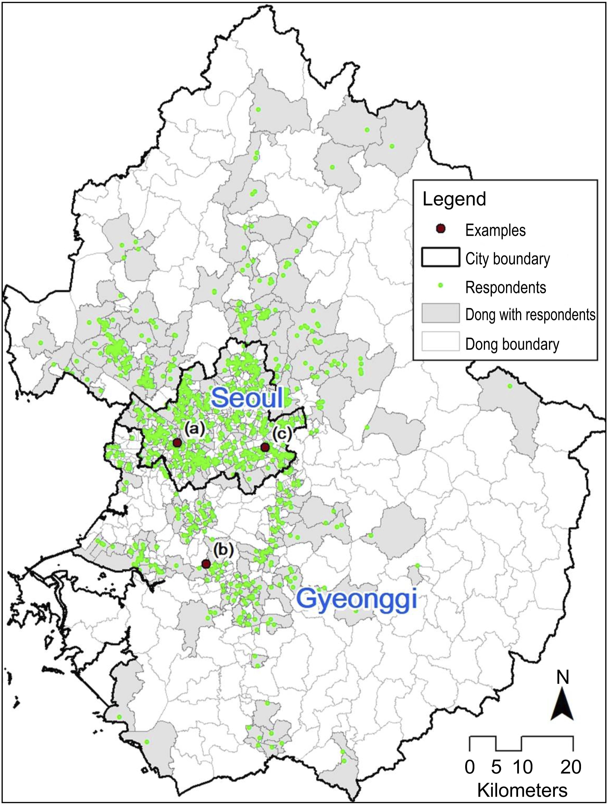

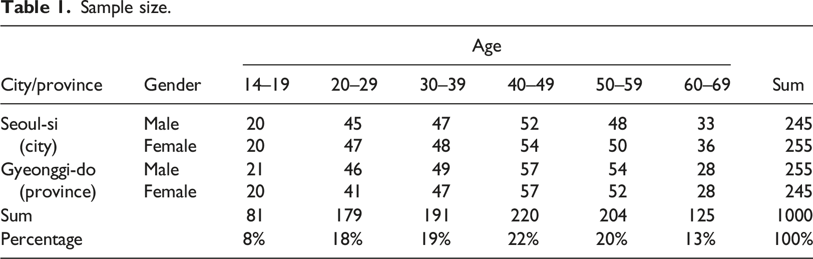
The CF survey, a structured online questionnaire to estimate CFs of residents, was conducted in Seoul and its suburb province, Gyeonggi, the Republic of Korea, in September 2009 and February 2018. A quota sampling method was used in both locations to reduce bias caused by age, gender, and region. Five hundred samples out of 1237 (40.4%) questionnaire copies and 1000 samples out of 1508 (66.3%) questionnaire copies were completed in 2009 and 2018, respectively. The quota sample size of age and gender was set by the proportion of each subpopulation group based on the age and gender structures within each city and province as a whole. The sample size of each city and province was evenly divided by sub-regions to derive spatially heterogeneous samples throughout the study areas (Table 1).

Table 1.

Sample size.

City/province	Gender	Age						Sum
City/province	Gender	14–19	20–29	30–39	40–49	50–59	60–69	Sum
Seoul-si (city)	Male	20	45	47	52	48	33	245
Seoul-si (city)	Female	20	47	48	54	50	36	255
Gyeonggi-do (province)	Male	21	46	49	57	54	28	255
Gyeonggi-do (province)	Female	20	41	47	57	52	28	245
Sum		81	179	191	220	204	125	1000
Percentage		8%	18%	19%	22%	20%	13%	100%

The calculation of individual CFs was based primarily on the Korean Institute Center for Sustainable Development (KICSD) ecological footprint questionnaire, which followed the calculation method of the Global Footprint Network (GFN, 2009; Kim and Kim, 2013).

Individual-level ecological footprint surveys are prepared by international non-governmental organizations, including the World Wide Fund for Nature (WWF) and Global Footprint Network (GFN), which commonly contain items related to food, housing/travel energy, and consumption of goods/services.

These ecological footprint surveys have been developed by calculating the relative size of individual footprints based on the average per capita energy consumption of each sector of a country divided by the population; therefore, they should convey accurate statistical information about a country.

As GFN provides the national footprint accounts data for each country with a consumption land-use matrix, KICSD revised the questionnaire of the ecological footprint survey of GFN and measured individual ecological footprints by reflecting the currency of Korea and average individual consumption by sectors based on Korea’s national statistics.

Although CF can include direct and indirect carbon dioxide emissions embedded in the life stages of a product (Wiedmann and Minx, 2008), it is difficult to distinguish the effects of spatial planning factors on the consumption of products from other factors (Kim, 2015). Therefore, among the consumption categories of the ecological footprint, only direct carbon emissions from fossil fuel energy use for housing and travel were considered as the CFs of residents in this study for an intuitive interpretation.

Housing CF in summer (HCF) and winter (HCFw) was calculated based on the monthly use of electricity, liquefied natural gas (LNG), oil, and liquefied petroleum gas (LPG) in July–August and January–February, respectively, in units of metric tons of carbon dioxide (tCO₂) by multiplying the conversion factors equivalent to the carbon intensities of each energy source (Ewing et al., 2008). Travel CF (TCF) was calculated from the survey data of yearly trip distance by private car and public transportation for different types of trips, which may related to the residents’ CO₂ emissions (Ashik et al., 2022; Yang and Zhou, 2020; Zhang et al., 2022), including commuting, business, shopping, recreation, and so on (Table 2).

Table 2.

Measures of variables.

Variables	Measurement (unit)
Urban density (Urb_density)	Population per urban area of each dong [people/m²]
Residential density (Res_density)	Population per residential area of each dong [people/m²]
Job opportunity (Job_opp) [model 0, 1, 2]	Ratio of the number of employees to the population
Residential/urban area (Res_Urb_R) [model 3]	Ratio of residential to urban area of each dong
Service accessibility (Serv_acc)	Number of bus stops, subway stations, parks, village offices, hospitals, pharmacies, banks, convenience stores, markets, marts, and department stores within 400 m (5 min walk distance) from home
Income	Monthly income of individuals on average [from 1 to 6]
Housing carbon footprint (HCF, HCFw^a)	Monthly use of electricity, liquefied natural gas (LNG), oil, and liquefied petroleum gas (LPG) [tCO₂]
Travel carbon footprint (TCF)	Yearly trip distance by private car and public transportation for commuting, business, and shopping [tCO₂]
Carbon footprint (CF, CFw^a)	Sum of housing and travel footprint [tCO₂]

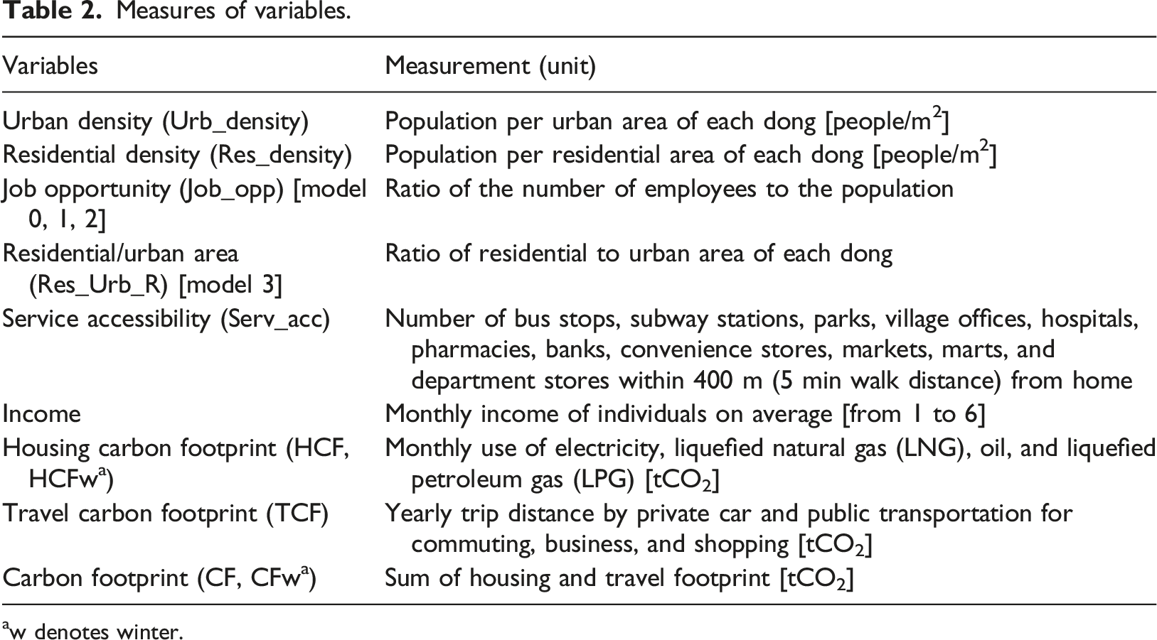
^aw denotes winter.

The survey questionnaire encouraged respondents to refer to monthly statements of utilities to reduce possible errors or uncertainties arising from self-report of consumption values for housing energy use in the summer (July and August) and winter (January and February) seasons. Concerning travel energy use, the public transportation fee of the city according to the travel distances and a city map with radial distances were provided as references for respondents to report the yearly mileage of personal vehicles and daily uses of public transportation.

The CF calculations in this study were for individuals, and some of the responses to the questions for the entire household, such as the monthly energy use for housing, were divided by the number of people sharing the house.

Spatial variables, such as urban/residential population densities and the ratio of residential to urban areas, were estimated by combining the statistics and electronic maps in geographic information system (GIS). The demographics, population, number of employees, and administrative boundary maps were provided by the Statistical Geographic Information Service (SGIS) (Statistics Korea, 2021b). Electronic maps of land-cover classification were provided by the Environmental Geographic Information Service (EGIS) (Ministry of Environment, 2021). The land-cover classification defined the urban area as a developed area with impermeable land uses, excluding cropland, forest, pasture, wetland, and water (Figure S1 in the Supplementary Material).

If the same number of people live in a dong, the lower the ratio of residential to urban areas, the higher the residential density [(b) → (a)], and more people live in a smaller area. However, if the residential density remains the same and the ratio of residential to urban areas increases, the population living in one dong also increases, thereby increasing the urban density [(a) → (c)] (Figure S1 in the Supplementary Material, Table 3).

Table 3.

Description of example areas.

	(a) 25% HL	(b) 50% LL	(c) 50% HH
Res_Urb_R	25% [24.6%]	50% [49.4%]	50% [50.4%]
Population	100 [16,844]	100 [14,672]	200 [21,680]
Res_density	100 (High) [45,871]	50 (Low) [19,067]	100 (High) [47,986]
Urb_density	25 (Low) [11,281]	25 (Low) [9423]	50 (High) [24,186]
# of samples	2	3	5
HCF	1.72	2.18	2.32
HCFw	3.26	2.47	2.25
TCF	1.60	0.61	2.65

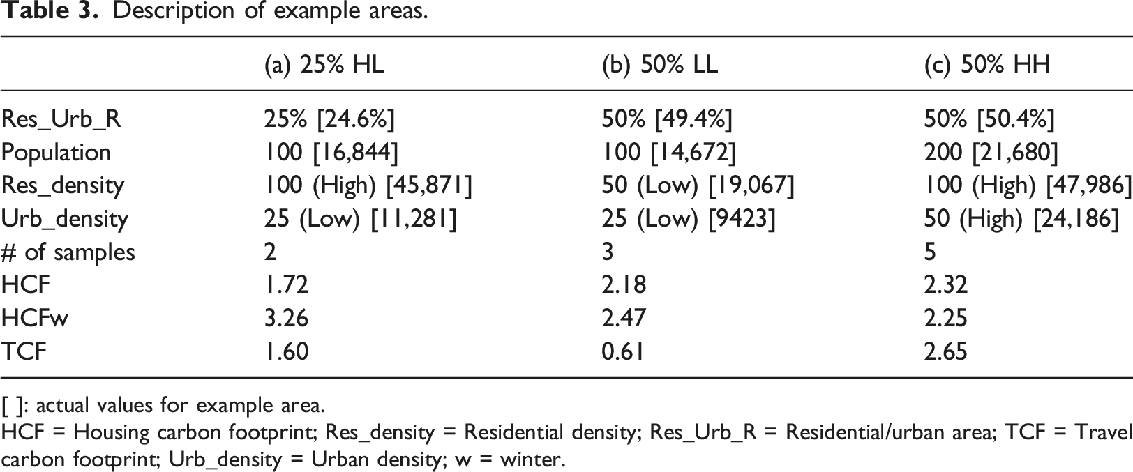
[ ]: actual values for example area.

HCF = Housing carbon footprint; Res_density = Residential density; Res_Urb_R = Residential/urban area; TCF = Travel carbon footprint; Urb_density = Urban density; w = winter.

As shown in Figure S2 in the Supplementary Material, the spatial distributions of the urban and residential densities of dongs, illustrated in five quantiles, are different from each other, even when the population of each dong is the same.

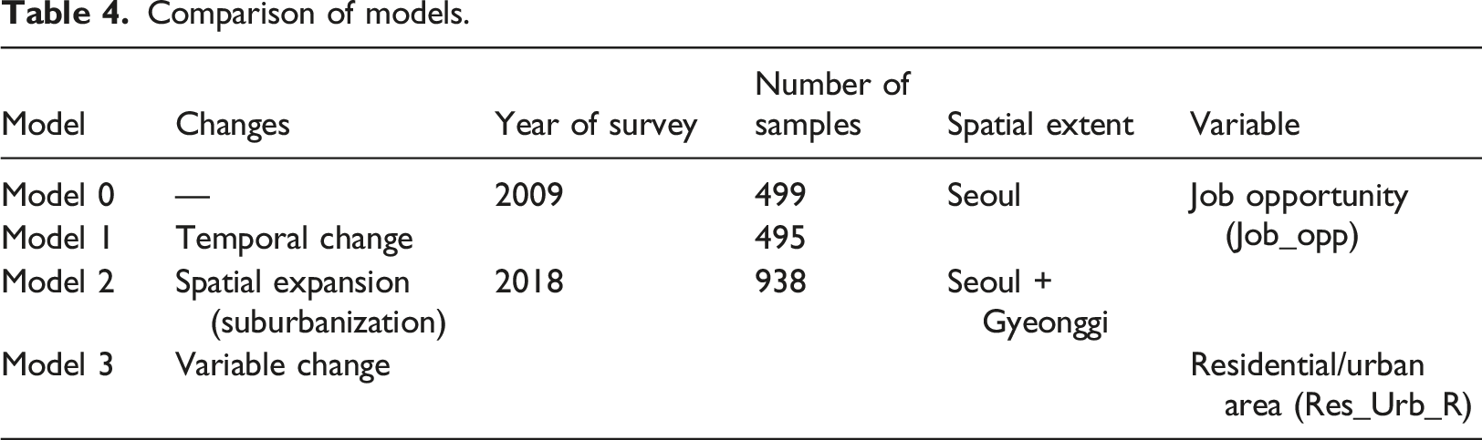
Four sets of path analyses were performed to verify the direct and indirect effects of spatial variables on residents’ CFs (Table 4, Figure 2).

Table 4.

Comparison of models.

Model	Changes	Year of survey	Number of samples	Spatial extent	Variable
Model 0	—	2009	499	Seoul	Job opportunity (Job_opp)
Model 1	Temporal change	2009	495	Seoul	Job opportunity (Job_opp)
Model 2	Spatial expansion (suburbanization)	2018	938	Seoul + Gyeonggi
Model 3	Variable change	2018	938	Seoul + Gyeonggi	Residential/urban area (Res_Urb_R)

Figure 2.

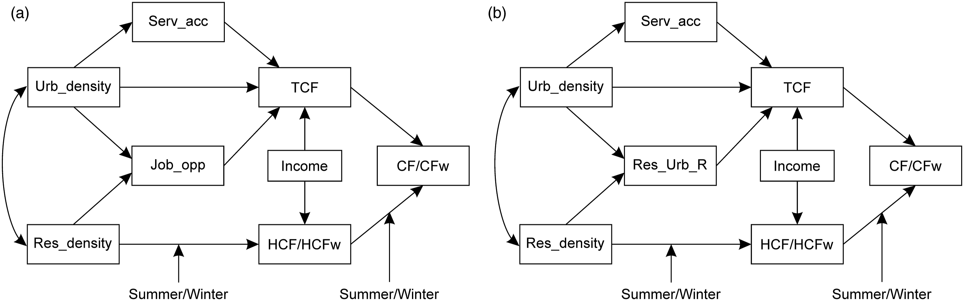
Structural equation models. (a) Model 0, 1, 2. (b) Model 3. CF = Carbon footprint; HCF = Housing carbon footprint; Res_density = Residential density; Res_Urb_R = Residential/urban area; TCF = Travel carbon footprint; Urb_density = Urban density; w = winter.

The limitations of simple regression analysis mean it is not sufficient for recognizing connections and associating independent variables in a model (Holden and Norland, 2005). Therefore, path analysis, structural equation modeling with observed variables, is frequently used in current research because it allows researchers to verify numerous relationships concurrently within the same analysis (Kim et al., 2010) and to examine the mediation and moderation of models easily (Kim and Kim, 2013).

The limitation of the path analysis method is that it requires a large number of cases to retain the precision of the estimates. However, the limitation might have less impact on this study because sufficient sample sizes have been collected following the benchmarking study. Many studies use 250‒500 samples for structural equation modeling, which is 10–20 times the number of model parameters (Schumacker and Lomax, 2004).

Path analysis with a set of mediation variables enables the evaluation of possible trade-offs, or co-benefits, when investigating the impacts of different measures of intra-urban densities and mixed land-use patterns on the CFs of the housing and travel sectors. Furthermore, the moderating effects of different cooling and heating patterns in different seasons on CFs were verified by comparing the four path analysis models in different spatiotemporal contexts.

First, in Models 0 through 2 the four predictors urban density, residential density, service accessibility, and job opportunity, and one control variable, income, were incorporated following the main hypothesis of previous work (Kim and Kim, 2013). The main hypothesis of this model was that urban density and residential density directly affect the TCF and HCF/HCFw. To verify the indirect effects of urban and residential densities on travel CF, service accessibility and job opportunities were incorporated as parameters mediating the effects. Seasonal differences in housing CF were considered to moderate the effects of residential density on HCF/HCFw and the contribution of HCF/HCFw to CF/CFw.

In Model 1, the model structure, number of samples (500 residents), and extent of spatial boundary (the city of Seoul) were the same as in Model 0, but the number of samples and year of data collection differed. The CF data of 495 residents of Seoul in 2018 were analyzed in Model 1, whereas 499 samples collected from the same city boundary in 2009 were analyzed in Model 0.

Model 2 had the same model structure as Model 1; the number of samples was doubled to 1000 residents, and the spatial boundaries were expanded to Gyeonggi-do, surrounding the outskirts of Seoul. A total of 938 out of 1000 samples were used for path analysis; 62 samples were excluded because they had no relevant demographic or spatial data.

Model 3 had the same conditions as Model 2 and one of the variables, Job opportunity, was substituted for a new spatial variable, the ratio of residential area to urban area. Job opportunities did not show a statistically significant relationship with TCF in Models 1 and 2. Further details are provided in the following sections. Models 1, 2, and 3 shared the same CF survey data from 2018, whereas Model 0 used 2009 CF survey data.

Results and discussion

Descriptive statistics

Descriptive statistics of the variables for each dataset are presented (Table 5).

Table 5.

Descriptive statistics of variables.

Dataset		2009 Seoul		2018 Seoul		2018 Seoul + Gyeonggi
Variables	Units	Mean	Std. Deviation	Mean	Std. Deviation	Mean	Std. Deviation
Area	km²	1.37	1.65	1.60	1.78	6.22	13.36
Urb_area	km²	0.82	0.52	0.85	0.42	1.37	1.66
Res_area	km²	0.40	0.20	0.44	0.18	0.47	0.35
Res_Urb_R	%	54.93%	18.37%	56.12%	16.41%	45.24%	20.89%
Workers	Person	5695.56	7520.08	12,900.43	18,846.23	12,426.43	17,150.67
Population	Person	23,271.64	8136.49	25,017.64	8968.08	28,674.85	14,792.73
Job_opp	%	25.76%	29.13%	61.96%	152.60%	52.03%	116.84%
Adm_density	Person/km²	26,473.29	15,303.43	23,101.53	11,098.03	17,352.58	12,179.85
Urb_density	Person/km²	34,118.17	14,631.40	32,944.32	12,071.82	29,871.11	18,896.73
Res_density	Person/km²	64,678.85	27,143.64	67,866.10	170,206.37	95,914.09	252,280.82
Serv_acc	Number	3.77	2.737	3.70	2.495	3.62	2.497
Age	Year	39.24	10.288	41.33	14.205	41.14	14.118
Income	Million ₩	3.58	1.563	4.34	1.469	4.39	1.444
HCF	tCO₂	1.95	0.85	2.32	1.06	2.26	1.05
HCFw	tCO₂	2.35	1.05	2.80	1.35	2.68	1.28
TCF	tCO₂	1.89	1.78	1.48	1.42	1.69	1.60
CF	tCO₂	3.83	2.06	3.80	1.84	3.95	1.96
CFw	tCO₂	4.23	2.13	4.28	2.02	4.38	2.09

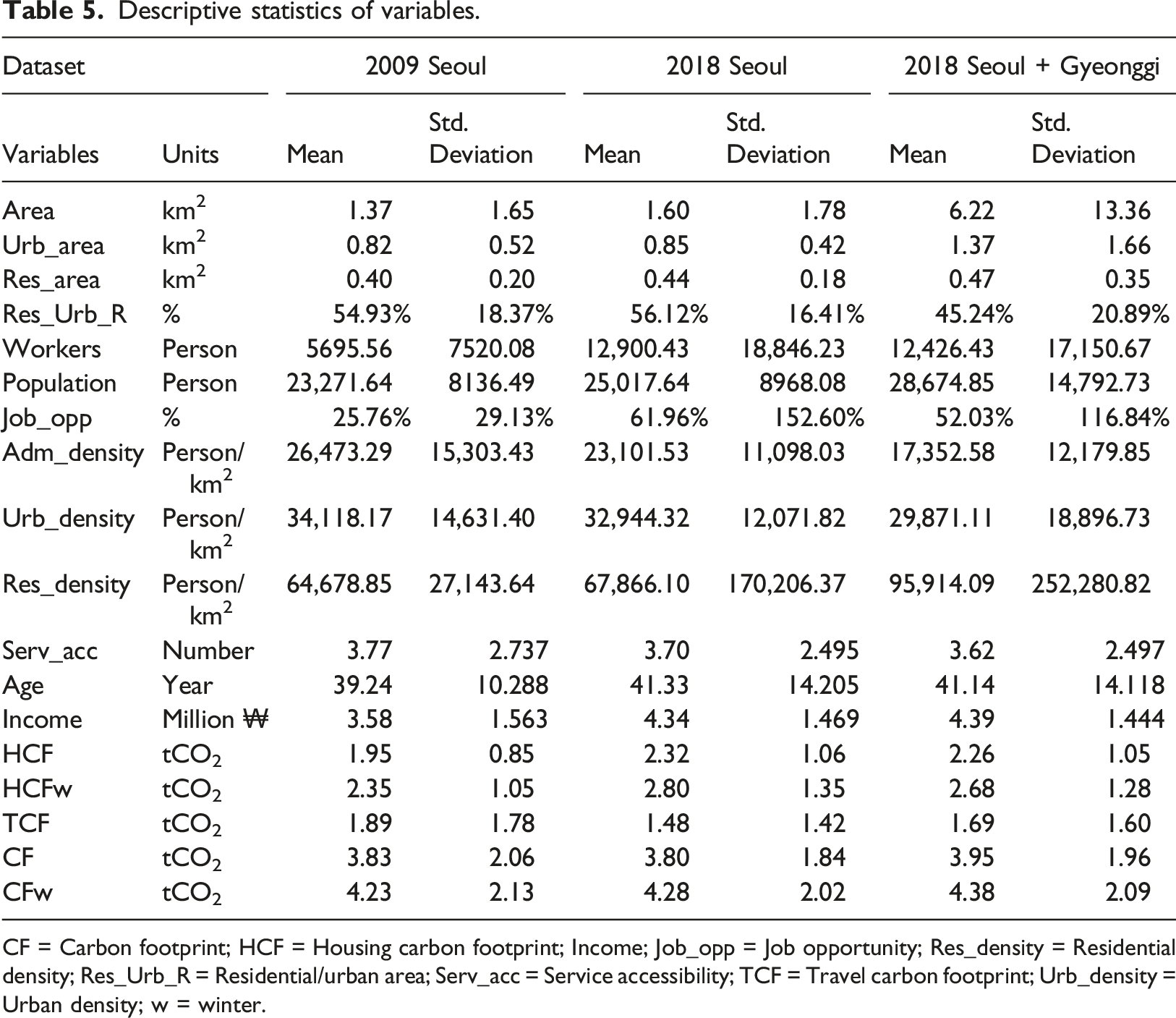
CF = Carbon footprint; HCF = Housing carbon footprint; Income; Job_opp = Job opportunity; Res_density = Residential density; Res_Urb_R = Residential/urban area; Serv_acc = Service accessibility; TCF = Travel carbon footprint; Urb_density = Urban density; w = winter.

The average administrative population density of each dong (Adm_density) and population density of urbanized regions (Urb_density) decreased from 2009 to 2018 in Seoul. In contrast, the average population density in residential areas (Res_density) showed an upward trend. The average Adm_density and Urb_density were lower in Gyeonggi than in Seoul, but the Res_density mean was higher with a large standard deviation.

The ratio of the number of workers to the population, representing job opportunities (Job_opp), increased from 2009 to 2018 in Seoul. In 2009 and 2018, the proportion of residential areas in the urbanized area (Res_Urb_R) of Seoul was 54.93% and 56.12%, respectively. The ratio of the combined areas in Seoul and Gyeonggi was 45.24% in 2018.

Model fit

The overall model fit indices showed that the model was reasonably consistent with the data. Table 6 shows that all model fit indices surpassed their acceptable values (Arbuckle, 2006; Kim, 2008; Kline, 2004; Lee and Lim, 2009).

Table 6.

Model fit indices.

Indices	Acceptable values (Arbuckle, 2006; Kline, 2004; Kim, 2008; Lee and Lim, 2009)	Obtained value
Indices		Model 0 [N = 499]	Model 1 [N = 495]	Model 2 [N = 938]	Model 3 [N = 938]
CMIN(χ²)	—	33.739	53.79	59.811	57.411
DF	—	32	32	32	32
CMIN/DF	<2	1.054	1.681	1.869	1.794
CFI	>0.9	1	0.994	0.996	0.997
PNFI	>0.5	0.567	0.564	0.567	0.568
PCFI	>0.5	0.571	0.568	0.569	0.57
RMSEA	<0.08	0.007	0.026	0.022	0.021
(HI 90)	(<0.08)	(0.025)	(0.038)	(0.03)	(0.029)

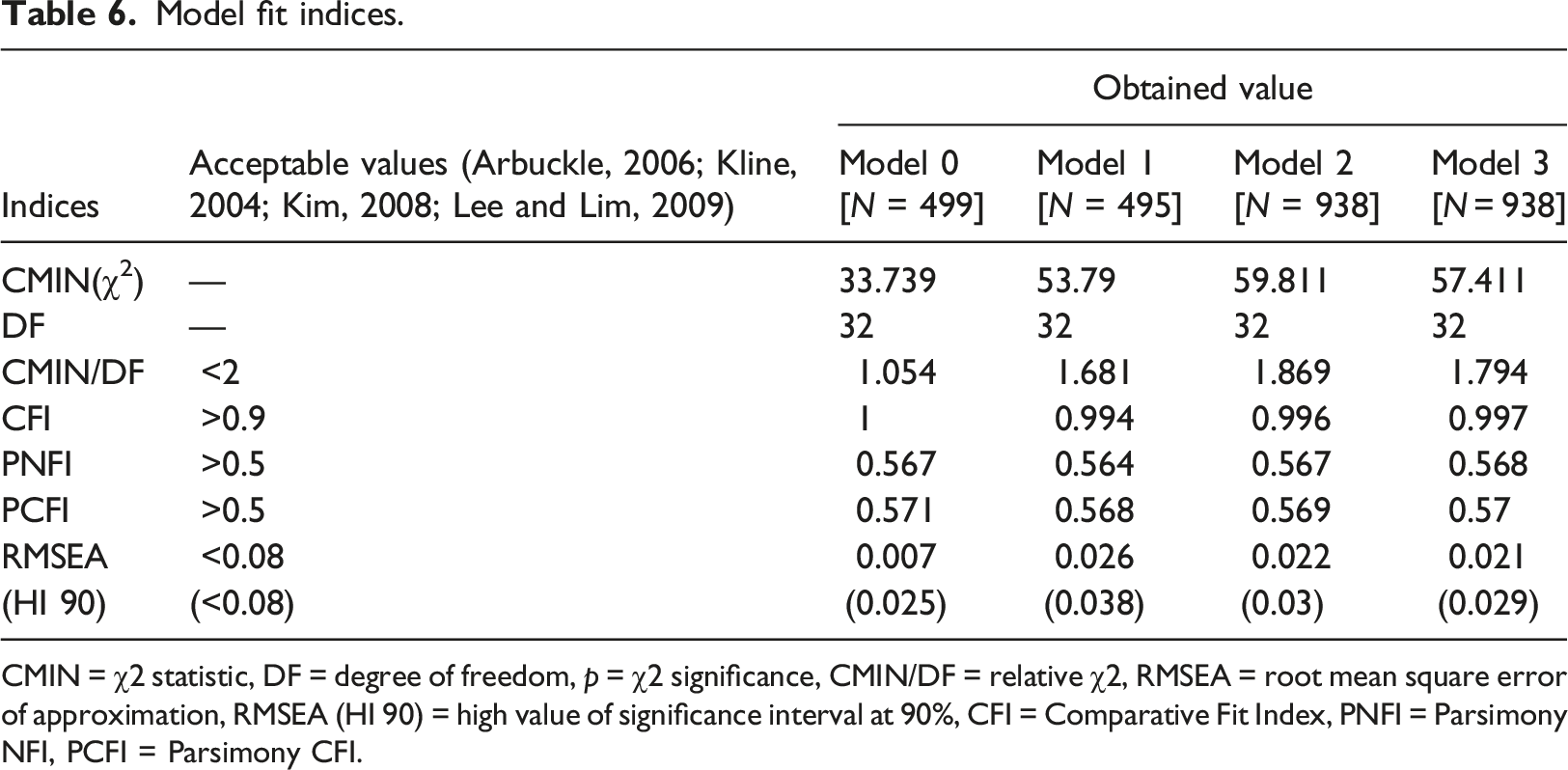
CMIN = χ2 statistic, DF = degree of freedom, p = χ2 significance, CMIN/DF = relative χ2, RMSEA = root mean square error of approximation, RMSEA (HI 90) = high value of significance interval at 90%, CFI = Comparative Fit Index, PNFI = Parsimony NFI, PCFI = Parsimony CFI.

Differences among models

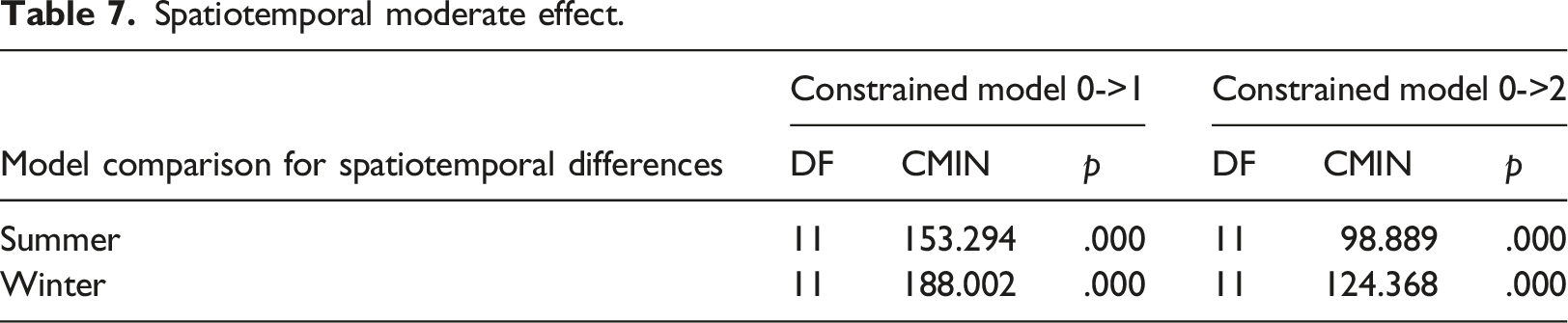
The differences between the CMIN values of the constrained and unconstrained models were statistically significant in both summer and winter (Table 7). This result means there is a difference in the path coefficient for each model, representing the temporal change in the data from Model 0 to Model 1 and the expansion of the spatiotemporal range from Model 0 to Model 2.

Table 7.

Spatiotemporal moderate effect.

Model comparison for spatiotemporal differences	Constrained model 0->1			Constrained model 0->2
Model comparison for spatiotemporal differences	DF	CMIN	p	DF	CMIN	p
Summer	11	153.294	.000	11	98.889	.000
Winter	11	188.002	.000	11	124.368	.000

Estimates of the standardized regression weights are shown in Table 8 and are represented in parentheses with statistical significance levels in the following text.

Table 8.

Estimates of standardized regression weights.

Exogenous variable	Endogenous variable	Estimates of standardized regression weights
Exogenous variable	Endogenous variable	Model 0 [N = 499]	Model 1 [N = 495]	Model 2 [N = 938]	Model 3 [N = 938]
Urb_density	Serv_acc	−0.016	−0.022	0.057*	0.057*
Urb_density	Job_opp	−0.621***	−0.478***	−0.408***	—
Res_density	Job_opp	0.22***	0.2***	0.254***	—
Urb_density	Res_Urb_R	—	—	—	0.932***
Res_density	Res_Urb_R	—	—	—	−0.908***
Job_opp	TCF	−0.054	−0.07	−0.034	—
Res_Urb_R	TCF	—	—	—	−0.121***
Serv_acc	TCF	−0.093**	−0.011	−0.058*	−0.059*
Income	TCF	0.221***	0.259***	0.225***	0.217***
Income	HCF	0.116***	−0.058	−0.028	−0.028
Income	HCFw	0.09**	−0.1**	−0.08**	−0.08**
Urb_density	TCF	−0.088*	−0.06	0.005	0.049
Res_density	HCF	−0.038	−0.053	−0.038	−0.038
Res_density	HCFw	−0.09**	−0.103**	−0.064**	−0.064**
TCF	CF	0.853***	0.774***	0.81***	0.81***
TCF	CFw	0.823***	0.699***	0.753***	0.754***
HCF	CF	0.473***	0.616***	0.559***	0.56***
HCFw	CFw	0.523***	0.707***	0.642***	0.643***

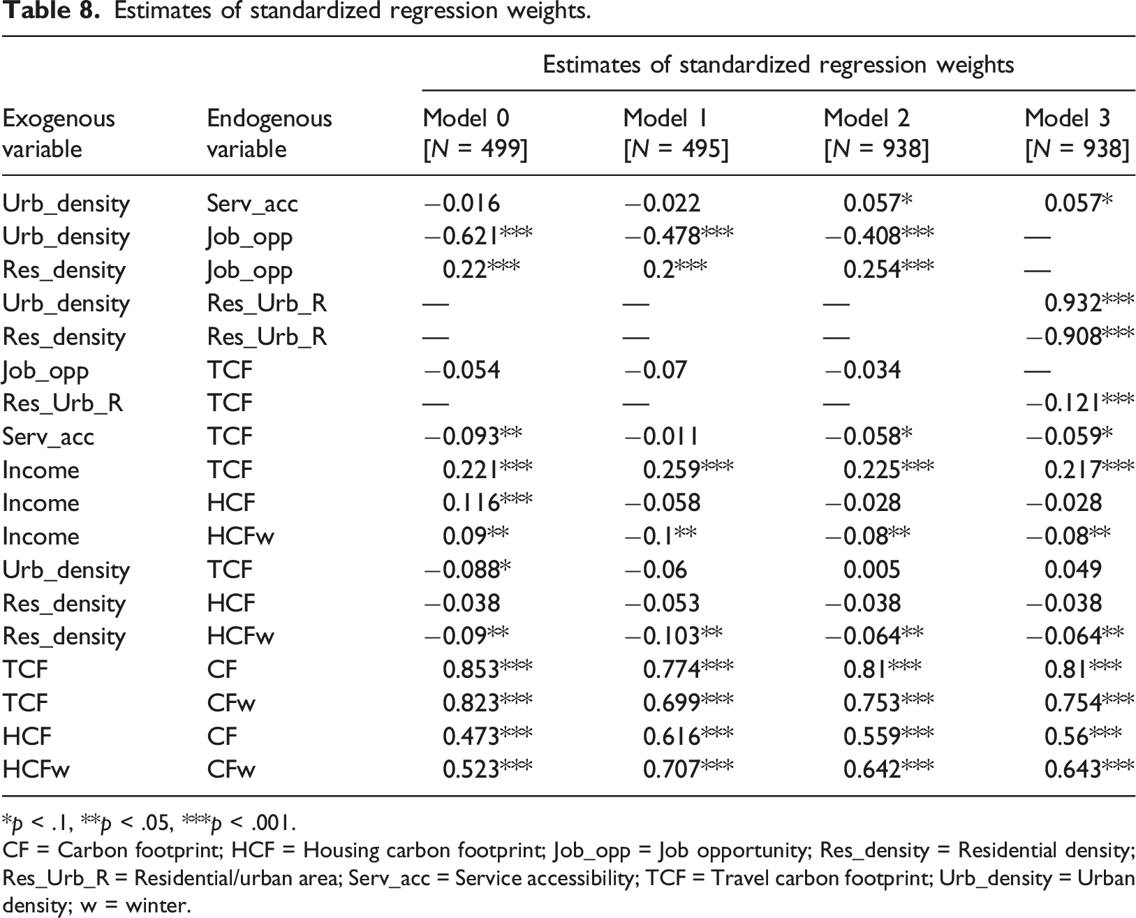
*p < .1, **p < .05, ***p < .001.

CF = Carbon footprint; HCF = Housing carbon footprint; Job_opp = Job opportunity; Res_density = Residential density; Res_Urb_R = Residential/urban area; Serv_acc = Service accessibility; TCF = Travel carbon footprint; Urb_density = Urban density; w = winter.

Spatiotemporal changes in urban density

While Model 0 showed that high urban density directly affected the reduction of TCF, the relationship between service accessibility and TCF became statistically insignificant in Model 1 (−0.011, p > .1) as the population density of Seoul decreased from 2009 to 2018. On the other hand, with the expansion of the spatiotemporal range, Model 2 demonstrated the indirect effect of high urban density on reducing TCF (−0.058*) by enhancing service accessibility (0.057*).

In dense urban areas, residents have a greater chance of accessing local services at walking distances, which may reduce the need for vehicle use. These significant relationships among the variables may have been influenced by suburbanization and population density growth in the suburbs between 2009 and 2018. Consequently, more urban areas with low TCFs for residents are likely to occur in the suburbs.

The impact of high urban density on reducing TCF contrasts with the urban heat island impact, which may increase HCF in conditions of high residential density, as other studies have shown. The trade-offs between the impacts of urban and residential densities on TCF and HCF are illustrated in the following sections.

Changes in parameters between urban density and TCF

Although the parameter Job opportunity was expected to affect the travel footprint, it had no statistically significant relationship with TCF in Models 0 (−0.054), 1 (−0.07), and 2 (−0.034). This seems to be because most of the respondents, 78.4% (392 out of 500) in 2009 Seoul and 77.1% (771 out of 1000) in Seoul and Gyeonggi in 2018, commuted to work or school in a different dong from the one in which they resided.

Therefore, in Model 3, the Job opportunity variable was replaced with the ratio of residential area to urban area (Figure 3).

Figure 3.

Model 3 results. (a) Summer. (b) Winter. CF = Carbon footprint; HCF = Housing carbon footprint; Res_density = Residential density; Res_Urb_R = Residential/urban area; Serv_acc = Service accessibility; TCF = Travel carbon footprint; Urb_density = Urban density; w = winter.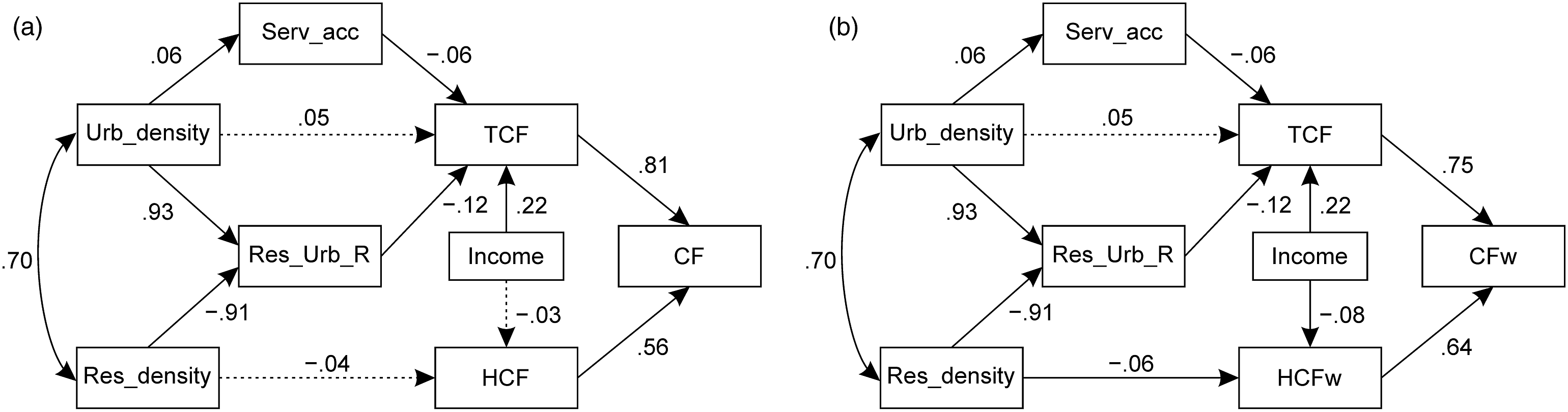

Different impacts of urban and residential densities on TCF

Areas with high urban density had high values of service accessibility (0.057*) and the ratio of the residential area to the urban area (0.932***) reduced TCF (−0.059*, −0.121***). In contrast, areas with high residential density eventually increased the TCF of residents because these areas had a low ratio of residential areas (−0.908***), which negatively impacted TCF (−0.121***). The standardized total effects of residential density on TCF, or combined indirect effects, showed a positive value (0.110), which means that high residential density increased TCF by 11%. This finding conflicts with the hypothesis that a higher population density in a city unit leads to a lower use of energy for travel.

When interpreting these results, it is necessary to understand the concept and spatial structure of a compact city that ‘reduces urbanized areas and increases the proportion of green areas through high-density development. This study shows the need for land-use planning that considers the intra-urban spatial structure, which is the ratio and density of residential areas within an urbanized area.

Impacts of the ratio of residential to urban areas on TCF and HCF

According to the results of the path analysis, high urban density may reduce the TCF per capita by increasing service accessibility or the ratio of residential areas. However, high urban and residential densities with an increase in population within the same urban and residential areas, for example, due to redevelopment with high-rise apartment buildings [(b)->(c)], may increase TCF and HCF but reduce HCFw (Table 3, Figure S1 in the Supplementary Material).

On the other hand, increasing residential density by lowering the ratio of residential areas within the same urban area [(b)->(a)] could increase TCF and HCFw and reduce HCF.

The seasonal difference in HCF between the example areas of (a) and (c) may be due to the urban heat island impact reducing the energy demand for heating in winter and requiring more energy demand for cooling in summer. The impact may be greater in areas such as (c) rather than in (a) because of the higher ratio of residential areas with dense residential buildings.

Existing studies provide evidence that a higher population density leads to lower energy use for travel (Holden and Norland, 2005; Kuzmyak et al., 2006; Lombardi et al., 2012; Williams et al., 2000), housing (Qin and Han, 2013), and both travel and housing (Lee and Lee, 2014). It is important to note that even the low residential density area (b) showed a low resident TCF because of the high ratio of residential to urban areas. On the contrary, the areas with a high residential density and a low ratio of residential to urban areas (a) could have a high TCF.

Kim and Kim (2013) assumed that the low ratio of residential to urban areas associated with a high mixture of different land uses reduces TCF. On the contrary, according to Model 3, urban areas with a high ratio of residential to urban areas can also have low TCF under certain conditions; notably, the even distribution of residential areas in urban areas with high service accessibility. These results have important implications for land-use planning and design in intra-urban spatial structures.

Seasonal differences of the effects of residential density and HCF

The difference in the fit (CMIN) of the constrained and non-constrained models, summer and winter, was statistically significant regarding the contribution of the HCF to the CF. However, there were no significant differences in the relationship between the residential density and HCF in Models 1, 2, and 3 (Table 9). These results are consistent with a previous study (Kim and Kim, 2013).

Table 9.

Seasonal moderate effect.

Model comparison for seasonal differences	Constrained model 1 (Res_density - > HCF)			Constrained model 2 (HCF - > CF)
Model comparison for seasonal differences	DF	CMIN	p	DF	CMIN	p
Model 1	1	0.756	.384	1	13.806	.000
Models 2, 3	1	0.371	.542	1	17.304	.000

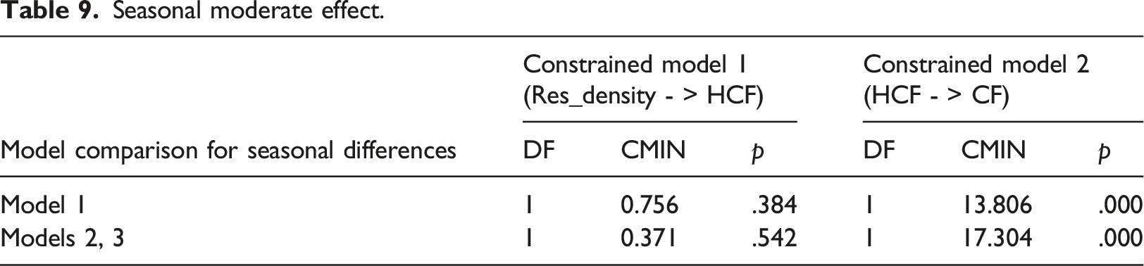
It is clear from all the models that, in contrast to summer, high residential density has a statistically significant relationship with low HCF in winter (Table 9). In addition, the share of the residential footprint affecting CF is greater in winter than in summer (HCF < HCFw in Models 0, 1, 2, and 3).

This result supports the need to analyze the relationship between density and CF with respect to different environmental and urban structural conditions, for example, temperature, humidity, rainfall, major housing types, and compactness of the city. In this study, the results suggest that it is necessary to focus on the energy demand for heating in winter rather than cooling in summer to reduce the carbon footprint in planning and design in cities such as Seoul and its metropolitan area. In winter, the individual HCF is lower in higher-income households. There was a positive relationship between household income, house size, and the number of people living together. It can be presumed that the individual HCF, which is divided from the HCF of an entire household, is relatively low because of multiple residents sharing the house and energy. Household income levels have a linear correlation with a household’s HCF, but the per capita HCF divided by the number of household members draws a parabola (Kim, 2015).

Conclusions

In this study, based on the results of the residents' carbon footprint surveys in the Seoul metropolitan area from 2009 to 2018, we analyzed how population density, job opportunities, land use, and service accessibility were related to the carbon footprints of residents.

This study fills a gap in previous studies that analyzed the relationship between urban spatial structure and residents’ carbon footprint by 1) verifying the difference in the relationship between variables temporarily, 2) expanding the spatial scope from the city boundary to the suburban areas, and 3) introducing a land-use variable, the ratio of residential to urban areas, to understand the relationship between energy use, density, and spatial structures. In addition, the study expanded the spatiotemporal scope of the analysis and revealed the relationship between urban spatial structure and housing carbon footprint through model specifications.

Consequently, spatiotemporal differences between the models were confirmed. Compared to a previous study by Kim and Kim (2013), service accessibility did not show the benefit of reducing TCF in 2018 in Seoul (Model 1). However, it was positively related to urban density and decreased the TCF in the greater metropolitan areas of Seoul and Gyeonggi. These differences derived from spatiotemporal changes among the models may reflect the impact of suburbanization on the relationships between the spatial structures and TCFs of residents. This implies that planning efforts to reduce TCF by enhancing service accessibility would be more effective in suburban areas than in the core city during suburbanization.

The results explain why the population density in urban and residential areas had opposite relationships to job opportunities and how job opportunities affect CFs. The proportion of residential land use in urban areas may be a key factor affecting CF.

Notably, a high residential to urban areas ratio is related to a low TCF, but its relationships with urban and residential densities show opposite outcomes. If urban areas have a low percentage of residential land use, the TCF of residents living in high-density residential areas is not necessarily low. Such a redevelopment replacing low-rise housing with high-rise apartment buildings without securing residential areas may increase total CF throughout the year due to the significant increase in TCF as well as the increase in HCF in summer, which offsets the slight decrease in HCF in winter.

The seasonal differences in the impact of residential density on HCF and their contribution to CFs were also significant. The impact of high residential density on reducing HCF was identified only in winter, and the contribution of HCF to CF was higher in winter. These values were constant in all models, regardless of the spatiotemporal changes. These results may support previous research (Ichinose et al., 1999), which verified the effects of urban heat islands in high-density cities, reducing housing energy demand in winter.

The compact city concept should be adopted carefully with respect to residential land use in intra-urban spatial planning due to trade-offs or co-benefits for HCF and TCF from particular urban forms and planning measures. Our study results have important implications for land-use planning and design in intra-urban spatial structures.

The study has some limitations, such as failure to survey the same respondents over time, limiting the study area to the metropolitan area of Seoul, and the inability to include other spatial variables, such as land-use complexity, in the models. In addition, structure equation modeling has limitations because it is dependent on a priori specification and cannot identify effects unless a pathway has been specified a priori (i.e., it can be misleading if the model specification is inaccurate).

Despite these limitations, this study can inform future research agendas. Our study showed the varied effects of urban structures on CFs. Different land-use types and structural densities can lead to contradictory results, even under the same population density. Attempts to reveal the effect of land-use complexity can be a starting point for analyses and can lead to other structural conditions. Future research agendas could be expanded to incorporate both locational and environmental conditions. Finding the optimal configuration of urban structures and density that lowers CFs would be a significant achievement for sustainable planning and urban design.

Supplemental Material

Supplemental Material - Planning factors affecting carbon footprints of residents: Density, land use, and suburbanization

Supplemental Material for Planning factors affecting carbon footprints of residents: Density, land use, and suburbanization by Taehyun Kim and Youngre Noh in Environment and Planning B: Urban Analytics and City Science

Footnotes

Declaration of conflicting interests

The author(s) declared no potential conflicts of interest with respect to the research, authorship, and/or publication of this article

Funding

The author(s) disclosed receipt of the following financial support for the research, authorship, and/or publication of this article: This paper is based on the findings of the research project “A Study on the Spatial Planning Factors of Smart Sustainable Cities Considering Ecological Footprints of Residents,” which was funded by the Korea Environment Institute (KEI) and “Analysis of Residents’ Ecological Footprint for Urban Restructuring in Low-growth Era,” (2017-029, 2018-018) which was conducted by the Korea Environment Institute (KEI) and funded by the Young Researcher Program (Project No. 2017R1C1B1012391) of the National Research Foundation of Korea.

ORCID iDs

Taehyun Kim

Youngre Noh

Supplemental Material

Supplemental material for this article is available online.

Taehyun Kim is a senior research fellow at Korea Environment Institute and was a visiting scholar at Texas A&M University and University of Arizona. His research interest focuses on sustainable and resilient environmental planning and design. His publications include applications of carbon footprint in urban planning and geography, assessments of local acceptance of radioactive waste facilities, spatio-temporal association of fossil fuel CO₂ emissions from crop production, relationship between pedestrian traffic volumes and built environment, and related topics.

Dr. Noh is an assistant professor at Texas A&M University. His research focuses on assessing the effects of physical planning on social equity, the environment, and housing by leveraging large data sets, including historical records. He has published several studies analyzing the long-term impact of planning decisions on housing values, evaluating various methods for measuring spillover effects, and exploring the cause and effect relationship between planning and the housing market.

References

Arbuckle

(2006) AMOS 7.0 User Guide. Chicago: SPSS.

Ashik

Rahman

Antipova

, et al. (2022) Analyzing the impact of the built environment on commuting-related carbon dioxide emissions. International Journal of Sustainable Transportation 17: 258–272.

Cao

Kang

, et al. (2019) Estimation and decomposition analysis of carbon emissions from the entire production cycle for Chinese household consumption. Journal of Environmental Management 247: 525–537.

Chen

Jia

Lau

SSY

(2008) Sustainable urban form for Chinese compact cities: Challenges of a rapid urbanized economy. Habitat International 32(1): 28–40.

Clarke

(2003) Urban planning and design. In: Thomas

(ed), Sustainable Urban Design: An environmental approach. London: Spon Press, pp. 14–24.

Dujardin

Marique

A-F

Teller

(2014) Spatial planning as a driver of change in mobility and residential energy consumption. Energy and Buildings 68(C): 779–785.

Ewing

Bartholomew

Winkelman

, et al. (2007) Growing Cooler: The Evidence on Urban Development and Climate Change. Washington, DC, Urban Land Institute

Ewing

Reed

Rizk

, et al. (2008) Calculation Methodology for the National Footprint Accounts. 2008 edition. Oakland: Global Footprint Network.

Ewing

Rong

(2008) The impact of urban form on U.S. residential energy use. Housing Policy Debate 19(1): 1–30.

10.

Ewing

Schmid

Killingsworth

, et al. (2003) Relationship between urban sprawl and physical activity, obesity, and morbidity. American Journal of Health Promotion 18(1): 47–57.

11.

Frenkel

Ashkenazi

(2008) The integrated sprawl index: measuring the urban landscape in Israel. The Annals of Regional Science 42(1): 99–121.

12.

GFN (2009) Ecological Footprint Standards 2009. Oakland: Global Footprint Network.

13.

Goldstein

Reames

Newell

(2022) Racial inequity in household energy efficiency and carbon emissions in the United States: An emissions paradox. Energy Research and Social Science 84: 102365. DOI: 10.1016/j.erss.2021.102365

14.

Gyeonggi-do Office (2021) Gyeonggi Statistics. Available at: stat.gg.go.kr (Accessed: 18 August 2021).

15.

Haddad

Aouachria

(2015) Impact of the transport on the urban heat island. International Journal of Environmental and Ecological Engineering 9(8): 968–973.

16.

Hamin

Gurran

(2009) Urban form and climate change: Balancing adaptation and mitigation in the U.S. and Australia. Habitat International 33: 238–245.

17.

B-J

Wang

Zhu

, et al. (2022) Beating the urban heat: Situation, background, impacts and the way forward in China. Renewable and Sustainable Energy Reviews 161: 112350. DOI: 10.1016/j.rser.2022.112350

18.

Holden

Norland

(2005) Three challenges for the compact city as a sustainable urban form: Household consumption of energy and transport in eight residential areas in the Greater Oslo Region. Urban Studies 42: 2145–2166. DOI: 10.1080/00420980500332064

19.

Hong

Hui

Lin

(2022) Relationship between urban spatial structure and carbon emissions: A literature review. Ecological Indicators 144: 109456. DOI: 10.1016/j.ecolind.2022.109456

20.

Huo

Cai

, et al. (2021) Will the urbanization process influence the peak of carbon emissions in the building sector? A dynamic scenario simulation. Energy and Buildings 232: 110590. DOI: 10.1016/j.enbuild.2020.110590

21.

Ichinose

Shimodozono

Hanaki

(1999) Impact of anthropogenic heat on urban climate in Tokyo. Atmospheric Environment 33(24): 3897–3909. DOI: 10.1016/S1352-2310(99)00132-6

22.

Jones

Kammen

(2014) Spatial Distribution of U.S. household carbon footprints reveals suburbanization undermines greenhouse gas benefits of urban population density. Environmental Science and Technology 48(2): 895–902. DOI: 10.1021/es4034364

23.

Kim

(2008) Amos A to Z. Paju: Hakhyunsa.

24.

Kim

(2015) Applications of carbon footprint in urban planning and geography. In: Muthu

(ed), The Carbon Footprint Handbook. Boca Raton: CRC Press, pp. 163–182.

25.

Kim

(2013) Analysis of the effects of intra-urban spatial structures on carbon footprint of residents in Seoul, Korea. Habitat International 38: 192–198.

26.

Kim

Ahn

, et al. (2010) Suppression of lipopolysaccharide-induced microglial activation by a benzothiazole derivative. Molecules and Cells 30: 51–57.

27.

Kim

T-K

Kim

H-K

Han

S-K

(2011) An analysis of the effects of spatial features of neighborhood on households’ energy use for food, housing and travel - focused on the ecological footprint survey in gyeonggi-do. Journal of the Korea Planners Association 46(1): 117–127.

28.

Kline

(2004) Principles and practice of structural equation modeling. New York: Guilford Press.

29.

Kovács

Harangozó

Szigeti

, et al. (2020) Measuring the impacts of suburbanization with ecological footprint calculations. Cities 101: 102715. DOI: 10.1016/j.cities.2020.102715

30.

Kuzmyak

Baber

Savory

(2006) Use of walk opportunities index to quantify local accessibility. Transportation Research Record: Journal of the Transportation Research Board 1977: 145–153.

31.

Lee

H-S

Lim

J-H

(2009) Structural Equation Modeling with AMOS 16.0. Paju: Bobmunsa.

32.

Lee

(2014) The influence of urban form on GHG emissions in the U.S. household sector. Energy Policy 68: 534–549.

33.

Liao

Zhang

Zhao

, et al. (2022) Built environment factors (bef) and residential land carbon emissions (RLCE). Buildings 12(5): 508. DOI: 10.3390/buildings12050508

34.

Lin

Yuan

Yang

, et al. (2019) Impact of extreme meteorological events on ozone in the Pearl River Delta, China. Aerosol and Air Quality Research 19(6): 1307–1324.

35.

Liu

Tang

Chen

, et al. (2022) Urban sprawl and carbon emissions effects in city areas based on system dynamics: a case study of Changsha City. Applied Sciences 12(7): 3244. DOI: 10.3390/app12073244

36.

Lombardi

Leach

Rogers

, et al. (2012) Designing Resilient Cities. Garston: IHS BRE Press.

37.

Wang

Liang

, et al. (2021) Changing effect of urban form on the seasonal and diurnal variations of surface urban heat island intensities (SUHIIs) in more than 3000 cities in China. Sustainability 13(5): 2877.

38.

Ministry of Environment (2021) Environmental Geographic Information Service (EGIS). Available at: egis.me.go.kr (Accessed: 18 August 2021).

39.

Muñiz

Dominguez

(2020) The impact of urban form and spatial structure on per capita carbon footprint in U.S. larger metropolitan areas. Sustainability 12(1): 389. DOI: 10.3390/su12010389

40.

Newman

(2006) The environmental impact of cities. Environment and Urbanization 18(2): 275–295. DOI: 10.1177/0956247806069599

41.

(2009) Policies and technical guidelines for urban planning of high-density cities - air ventilation assessment (AVA) of Hong Kong. Building and Environment 44(7): 1478–1488.

42.

Oke

Mills

Voogt

(2017) Urban Climates. Cambridge, UK: Cambridge University Press.

43.

Owens

(1986) Energy, Planning and Urban Form. London, UK: Taylor and Francis.

44.

Owens

(1990) Land use planning for energy efficiency. In: Cullingworth

(ed), Energy, land and public policy. New Brunswick, NJ: Transaction Publishers.

45.

Owens

(1992) Energy, environmental sustainability and land-use planning. In: Breheny

(ed), Sustainable Development and Urban Form. London, UK: Pion, pp. 79–105.

46.

Qin

Han

(2013) Planning parameters and household carbon emission: evidence from high- and low-carbon neighborhoods in Beijing. Habitat International 37: 52–60. DOI: 10.1016/j.habitatint.2011.12.017

47.

Ramírez-Aguilar

Lucas Souza

(2019) Urban form and population density: influences on urban heat island intensities in Bogotá, Colombia. Urban Climate 29: 100497. DOI: 10.1016/j.uclim.2019.100497

48.

Rong

Zhang

Qin

, et al. (2020) Spatial differentiation of carbon emissions from residential energy consumption: a case study in Kaifeng, China. Journal of Environmental Management 271: 110895. DOI: 10.1016/j.jenvman.2020.110895

49.

Salamanca

Georgescu

Mahalov

, et al. (2014) Anthropogenic heating of the urban environment due to air conditioning. Journal of Geophysical Research: Atmospheres 119(10): 5949–5965. DOI: 10.1002/2013Jd021225

50.

Seoul Metropolitan Government (2021) Seoul Open Data Plaza. Available at: data.seoul.go.kr (Accessed: 18 August 2021).

51.

Schumacker

Lomax

(2004) A Beginner’s Guide to Structural Equation Modeling. Hillsdale, NJ: Lawrence Erlbaum.

52.

Shen

Y-S

Lin

Y-C

Cui

, et al. (2022) Crucial factors of the built environment for mitigating carbon emissions. Science of The Total Environment 806: 150864. DOI: 10.1016/j.scitotenv.2021.150864

53.

Shi

Liu

Cui

, et al. (2023) What urban spatial structure is more conducive to reducing carbon emissions? A conditional effect of population size. Applied Geography 151: 102855. DOI: 10.1016/j.apgeog.2022.102855

54.

Statistics Korea (2021a) e-National Indicators. Available at: www.index.go.kr (Accessed: 18 August 2021).

55.

Statistics Korea (2021b) Statistical Geographic Information Service (SGIS). Available at: sgis.kostat.go.kr (Accessed: 18 August 2021).

56.

Thornbush

Golubchikov

(2019) Sustainable Urbanism in Digital Transitions: From Low Carbon to Smart Sustainable Cities. Berlin: Springer.

57.

Wang

You

, et al. (2022) Gravity center change of carbon emissions in Chinese residential building sector: differences between urban and rural area. Energy Reports 8: 10644–10656. DOI: 10.1016/j.egyr.2022.08.208

58.

Wang

Zhan

, et al. (2019) Structural decomposition analysis of carbon emissions from residential consumption in the Beijing-Tianjin-Hebei region, China. Journal of Cleaner Production 208: 1357–1364. DOI: 10.1016/j.jclepro.2018.09.257

59.

Wiedenhofer

Smetschka

Akenji

, et al. (2018) Household time use, carbon footprints, and urban form: a review of the potential contributions of everyday living to the 1.5°C climate target. Current Opinion in Environmental Sustainability 30: 7–17. DOI: 10.1016/j.cosust.2018.02.007

60.

Wiedmann

Minx

(2008) A Definition of ‘Carbon Footprint’. In: Pertsova

(ed.) Ecological Economics Research Trends. Hauppauge NY, USA: Nova Science Publishers, 1–11.

61.

Williams

Burton

Jenks

(2000) Achieving Sustainable Urban Form. London: E and FN Spon.

62.

Williams

Joynt

JLR

Hopkins

(2010) Adapting to climate change in the compact city: the suburban challenge. Built Environment 36(1): 105–115. DOI: 10.2148/benv.36.1.105

63.

Frazier

(2021) Spatiotemporal variation and driving factors of carbon emissions in three industrial land spaces in China from 1997 to 2016. Technological Forecasting and Social Change 169: 120837. DOI: 10.1016/j.techfore.2021.120837

64.

Yang

Meng

(2020) Analysis of the decoupling effect and eco-economic coordination of the resident energy carbon footprint: a case study of Caijiapo Town, a national key town in western China. Environmental Science and Pollution Research 27(7): 6936–6949. DOI: 10.1007/s11356-019-07350-w

65.

Yang

Zhou

(2020) Using decision tree analysis to identify the determinants of residents’ CO2 emissions from different types of trips: a case study of Guangzhou, China. Journal of Cleaner Production 277: 124071. DOI: 10.1016/j.jclepro.2020.124071

66.

Zhang

Yuan

, et al. (2015) Mass human migration and Beijing’s urban heat island during the Chinese new year holiday. Science Bulletin 60(11): 1038–1041.

67.

Zhang

ZhouMohibi

DingVasilatis

, et al. (2022) Effects of the built environment on travel-related co2 emissions considering travel purpose: a case study of resettlement neighborhoods in Nanjing. Buildings 12(10): 1718–1726. DOI: 10.3390/buildings12101718

68.

Zheng

Huang

Sun

(2022) Effects of urban form on carbon emissions in china: implications for low-carbon urban planning. Land 11(8): 1343. DOI: 10.3390/land11081343

69.

Zhou

Rybski

Kropp

(2017) The role of city size and urban form in the surface urban heat island. Scientific Reports 7(1): 4791.

70.

Zhu

Chen

, et al. (2022) The spatial-temporal patterns and multiple driving mechanisms of carbon emissions in the process of urbanization: a case study in Zhejiang, China. Journal of Cleaner Production 358: 131954. DOI: 10.1016/j.jclepro.2022.131954

71.

Zubelzu

Álvarez Fernández

(2016) Carbon Footprint and Urban Planning: Incorporating Methodologies to Assess the Influence of the Urban Master Plan on the Carbon Footprint of the City. Cham, Switzerland: Springer International Publishing AG.

Supplementary Material

Please find the following supplemental material available below.

For Open Access articles published under a Creative Commons License, all supplemental material carries the same license as the article it is associated with.

For non-Open Access articles published, all supplemental material carries a non-exclusive license, and permission requests for re-use of supplemental material or any part of supplemental material shall be sent directly to the copyright owner as specified in the copyright notice associated with the article.

0.00 MB

0.08 MB

Planning factors affecting carbon footprints of residents: Density,land use,and suburbanization

Abstract

Keywords

Introduction

Urban density and residents’ CFs

Methods

Results and discussion

Descriptive statistics

Model fit

Differences among models

Spatiotemporal changes in urban density

Changes in parameters between urban density and TCF

Different impacts of urban and residential densities on TCF

Impacts of the ratio of residential to urban areas on TCF and HCF

Seasonal differences of the effects of residential density and HCF

Conclusions

Supplemental Material

Supplemental Material - Planning factors affecting carbon footprints of residents: Density, land use, and suburbanization

Footnotes

Declaration of conflicting interests

Funding

ORCID iDs

Supplemental Material

References

Supplementary Material