Sage Journals: Discover world-class research

Abstract

Implementing carbon mitigation through urban spatial optimisation is a possible solution for alleviating global warming. However, the relationship between urban carbon emissions and urban spatial structure has not been well clarified, as adequate mapping of high-spatial-resolution urban carbon emissions from different sectors (particularly residential sectors), a precondition to solving the problem, has yet to be achieved. This study proposes a hybrid method of mapping the spatial distribution of urban residential carbon emissions on a 1 km × 1 km scale using multi-source data and exemplifies it via a case study of the Chinese city of Suzhou. The purpose of using this method is to differentiate residential carbon emissions by commuter population and home-based population, as the time they spend at home differs. The mobile signalling data of Suzhou were used to identify commuter and home-based populations. The number and spatial distribution of these two groups were then calibrated by referring to land use and O-D data. Using calibrated data, the proportion of electricity consumed by the two groups in different residential districts across the city was calculated. Total urban residential carbon emissions were then proportionally allocated to 1 km × 1 km grids. By validating estimated data against the data from the Statistical Yearbook, we found that the proximity level is higher than 93%. Furthermore, comparing these outcomes against the results estimated by using NTL data and the size of the identified population as the proxy data, it was observed that the results estimated by the hybrid method are of higher accuracy and stability.

Keywords

High-spatial resolution mapping residential carbon emissions hybrid method mobile signalling data

Introduction

Carbon emissions are a key cause of global warming. Therefore, carbon mitigation is regarded as an imperative human action to alleviate the pressing global warming challenge. Large-scale human activity since industrialisation has consumed massive amounts of energy in a relatively short time, which has contributed tremendously to global carbon emissions, resulting in global warming (IPCC, 2014). Mapping the spatial distribution of carbon emissions with a high-spatial accuracy is a prerequisite for exploring the relationship between carbon mitigation and urban spatial restructuring. However, the primary means of achieving this thus far have been studies or policy implications that focus on the interpretation of aggregate carbon emissions on a national, provincial, or city scale, rather than the optimisation of the spatial subunits of cities from which emissions are generated. The challenge in formulating mitigation policies from the latter perspective is a lack of deep understanding of how urban spatial structures shape carbon emissions. This is a result of the fact that the spatial distribution of carbon emissions within a city cannot be easily mapped without large-scale, resource-consuming investigations (Bai et al., 2018). Therefore, it is necessary to explore modelling methods for mapping urban carbon emissions with higher spatial resolution and accuracy to circumvent this difficulty.

The primary methods of spatial mapping of urban carbon emissions fall into two types: top-down and bottom-up modelling. Regarding top-down modelling, the goal is to decompose the aggregate carbon emissions of the city into portions and allot them to smaller land plots proportionately by referring to a certain plot attribute. The data used to describe the plot attributes are called proxy data. The advantage of top-down modelling is its ability to save time and resources. To apply this approach, it is essential to ensure that the proxy data is accurate enough that it can denote the percentage of carbon emissions from the concerned plot as closely as possibly to reality. In contrast, the bottom-up approach requires a large-scale dataset of emission sources and their locational information. The total amount of emissions from each emission source is then calculated by considering the real energy consumed. For example, some scholars have used the statistics of the energy use intensity of different buildings to map building carbon emissions across a city, whereas others have used point emission source, gridded emission, and supplementary socioeconomic data to spatially map carbon emissions across China (Cai et al., 2018a, 2018b; Wu et al., 2018; Jing et al., 2018; Sharifi, A., et al., 2018). Generally, spatial mapping of urban carbon emissions based on this approach is highly accurate (Cai et al., 2018a, 2018b). However, constrained by the unavailability of detailed energy consumption data for specific emission resources, the bottom-up modelling approach cannot be implemented without large-scale surveys which can be unaffordable (Jing et al., 2018).

Based on the various types of human activities, carbon emissions can be generalised into four categories: industrial, commercial, transport, and residential. As industrial carbon emissions are determined by the technical processes of production lines, it is possible to use the energy consumption data of point-based sources directly to map emissions (Cai et al., 2018). Commercial carbon emissions can be estimated and spatially mapped by referring to large-scale building datasets because the commercial functionality of buildings is highly homogeneous in terms of energy consumption (Wu et al., 2018). Similarly, by using detailed traffic flows on city roads, transport carbon emissions can be well modelled and spatially mapped (Cai et al., 2020). By combining these two approaches, the UK 1 km × 1 km resolution emission map (https://naei.beis.gov.uk/data/) and the China High Resolution Emission Database (CHRED) have been developed. Their modelling methods are similar; for large industrial and commercial sources, emissions are compiled from surveys or a variety of official regulatory sources. For diffuse emission sources, distribution maps are generated using the appropriate surrogate statistics for each sector. The experiences of the United Kingdom and China indicate that the choice of surrogate statistics is the key to the accuracy of the distributed emission map, which influences the accuracy of the final emission map.

The estimation and spatial modelling of residential carbon emissions are commonly performed using building data and night-time light images as proxy data (Zhuo et al., 2015; Shi et al., 2016; Meng et al., 2014). However, the phenomenon of a high housing vacancy rate should not be overlooked because estimating carbon emissions by assuming that all XXX buildings are fully occupied is unreliable. Additionally, when modelling carbon emissions by referring to the digital number (the value of dn) extracted from night-time light images, the value of dn does not change proportionately with the density of light when it reaches its maximum. This means that the carbon emissions of sites with an excessive intensity of energy consumption cannot be estimated correctly. More importantly, night-time light images can only represent energy consumption during the night; the main drawback being that the energy used by home-based populations in daylight is not well represented (Xie and Weng., 2016; Cai et al., 2021).

One solution to the abovementioned issues is to use the spatial distribution of residents as the proxy data to estimate and model residential carbon emissions across the city (Cai et al., 2018). Compared to the methods presented above, this approach generally has better performance in terms of accuracy and stability. However, it is worth noting that the percentage of general commuters in daylight could vary, which may lead to differences in carbon emissions among different resident groups of the same size. As residential carbon emissions largely come from the energy (e.g. electricity or gas) used by people when they are at home, the quantity of residential carbon emissions needs to be estimated not only by the size of the population but also by the time they spend at home. The key to spatially mapping residential carbon emissions with higher accuracy is to differentiate time spent at home among different groups.

In summary, effective top-down modelling approaches have been proposed for spatially mapping industrial, commercial, and transport carbon emissions. Regarding the approach to mapping residential carbon emissions, what has been proposed is acceptable, but higher accuracy in both quantity and spatial resolution can be achieved if we can use the real time that people spend at home as proxy data in combination with specific locational information of the population. This study proposes a hybrid modelling method to spatially map residential carbon emissions using multi-source data, including mobile signalling data. The key is to identify home-based residents and regular commuter-working residents within all identified residential districts so that the time these two groups spend at home can be well differentiated. Taking Suzhou as an example, this study also illustrates how this method can be applied in practice and the level of accuracy and stability that it can achieve.

Materials and methods

Study area and data

The city selected for this case study is Suzhou, which is located in the Yangtze Delta and is expected to have a population of more than 10 million permanent residents in 2021. It consists of 6 districts (Figure S1 in the Supplementary Material). In 2021, the urbanisation rate was 81.93%. It has a comparatively competent economy, with a total GDP of 334.14 billion dollars and a per capita GDP of 26,231 dollars.

The key data used in this research included mobile signalling data covering a consecutive month, June 2019, in Suzhou, land-use data of Suzhou extracted from the China land-use dataset, night-time light image data (raster data with a resolution of 30 m × 30 m) of Suzhou in 2019, and other socioeconomic data from the Statistical Yearbook of Suzhou (2020) (Table 1). The mobile signalling data with personal information erased was pre-processed before we received it. The following rules of processing were applied: 8:00 a.m. to 8:00 p.m. was considered working time, 8:00 p.m. to 8:00 a.m. was considered rest time, the base station that the user stopped at for the longest working time (8 h) in a day and repeated for more than 9 days was identified as the working place of the user, and the base station that the user stopped at for the longest rest period (8 h) in a day and repeated for more than 9 days was identified as the residence of the user. Each signalling dataset contains the location number and corresponding coordinates of the base station at the workplace, location number and corresponding coordinates of the base station at the residence, statistical number of people sharing the same workplace, base station at the residence, and other information. For people without a fixed workplace (such as couriers and insurance workers), only the location of the base station at the residence was recorded. Ultimately, 9.0253 million individuals were identified. This dataset was used to identify the total number of residents and regular commuter-working residents in each district (Gong et al., 2020; Lai et al., 2022; Zhang et al., 2020). Considering that the population of Suzhou is approximately 10 million, it is reasonable to assert that the use of mobile signalling data to identify the population and their location is highly representative. The land-use data includes five land-use types in Suzhou: residential, commercial, industrial, transport, and public administration and services. These details were used to calibrate the total number of residents and regular commuter-working residents, as identified using mobile signalling data at the first step in each statistical unit. By referring to the Statistical Yearbook, the electricity consumed by the urban and rural residents of each municipal district and county in Suzhou in 2019 was acquired. It is worth noting that statistical data of domestic gas consumption at a regional or smaller scale could not be obtained, and the results could not be verified; therefore, the gas data were not included in the model. However, because most residential carbon emissions come from electricity consumption by people staying at home, it is reasonable to use the percentage of electricity consumed by a person to denote the percentage of residential carbon emissions generated by that person. A night-time light image of Suzhou was used to map residential carbon emissions, against which the accuracy and stability of the mapping results obtained by the hybrid method were checked. It is also worth noting that the final spatial resolution of the mapped residential carbon emissions is 1 km × 1 km. The reason for this is that most communication base stations in Suzhou are 4G base stations with a signal coverage range of approximately 200–1200 m. Therefore, merging all the data into 1 km × 1 km grids can help improve the accuracy of the locational information of the identified population as well as residential carbon emissions.

Table 1.

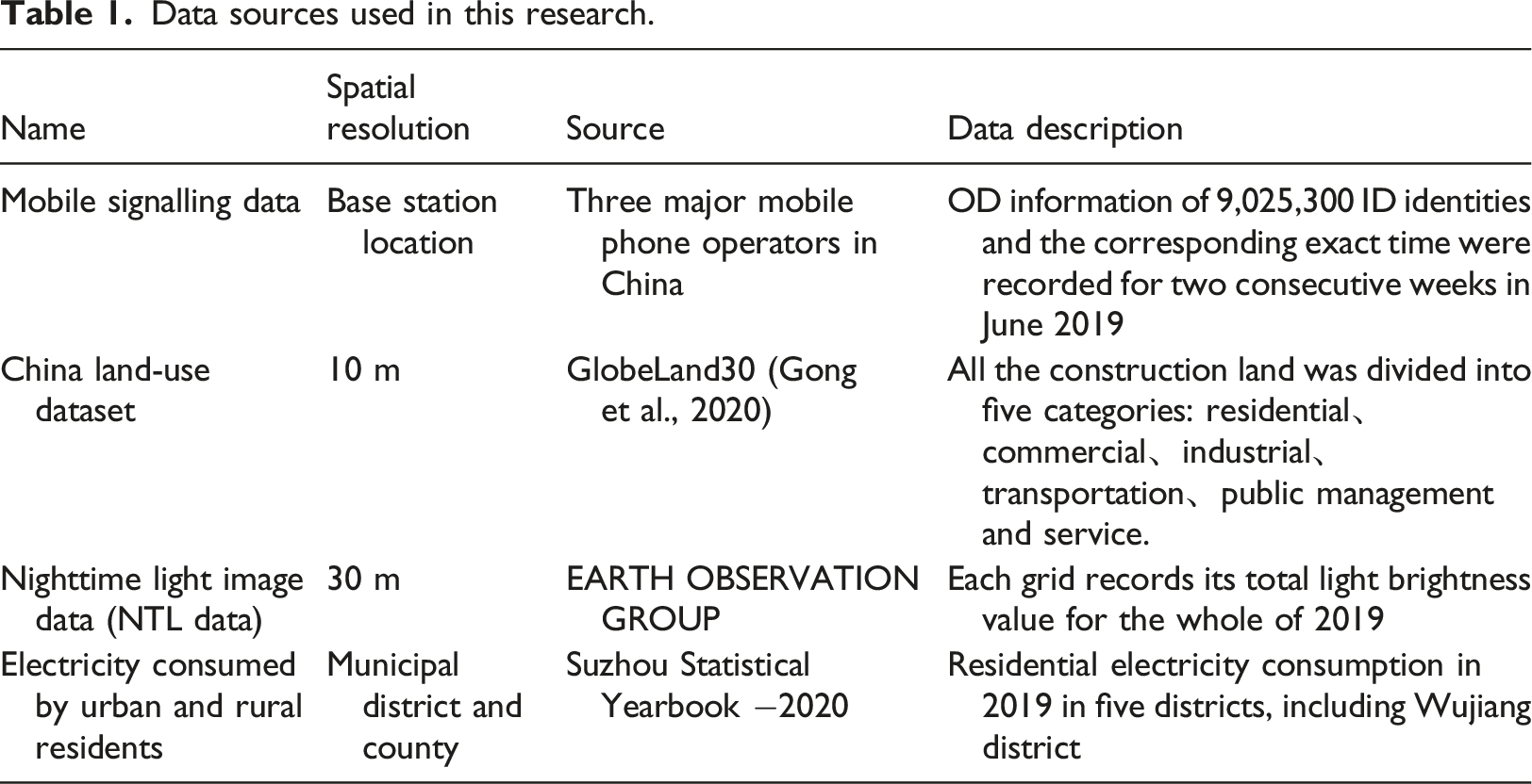
Data sources used in this research.

Name	Spatial resolution	Source	Data description
Mobile signalling data	Base station location	Three major mobile phone operators in China	OD information of 9,025,300 ID identities and the corresponding exact time were recorded for two consecutive weeks in June 2019
China land-use dataset	10 m	GlobeLand30 (Gong et al., 2020)	All the construction land was divided into five categories: residential、commercial、industrial、transportation、public management and service.
Nighttime light image data (NTL data)	30 m	EARTH OBSERVATION GROUP	Each grid records its total light brightness value for the whole of 2019
Electricity consumed by urban and rural residents	Municipal district and county	Suzhou Statistical Yearbook −2020	Residential electricity consumption in 2019 in five districts, including Wujiang district

Research framework

The research framework for this study is illustrated in Figure 1. The key to the hybrid modelling method is to determine the correct proxy data so that the total residential carbon emissions can be reasonably decomposed and assigned to each spatial grid. Therefore, the first step in this research was to calculate the proxy data, that is, the time spent at home by home-based residents (N_home) and regular commuter-working residents (N_commute). To do this, first the spatial distribution of the population within Suzhou was identified using the mobile signalling data. This population distribution map was then calibrated by referring to the land-use map of Suzhou so that the number of home-based residents and regular commuter-working residents in each grid could be differentiated and acquired. Assuming that the time spent at home by these two groups differed, the total time spent by all residents at home in each grid (1 km × 1 km) was calculated. The total time was then used to estimate the percentage of residential carbon emissions that each grid took up. Therefore, the total residential carbon emissions for the entire city of Suzhou can be decomposed and assigned to each grid proportionately according to the corresponding percentage that it shares.

Figure 1.

The research framework.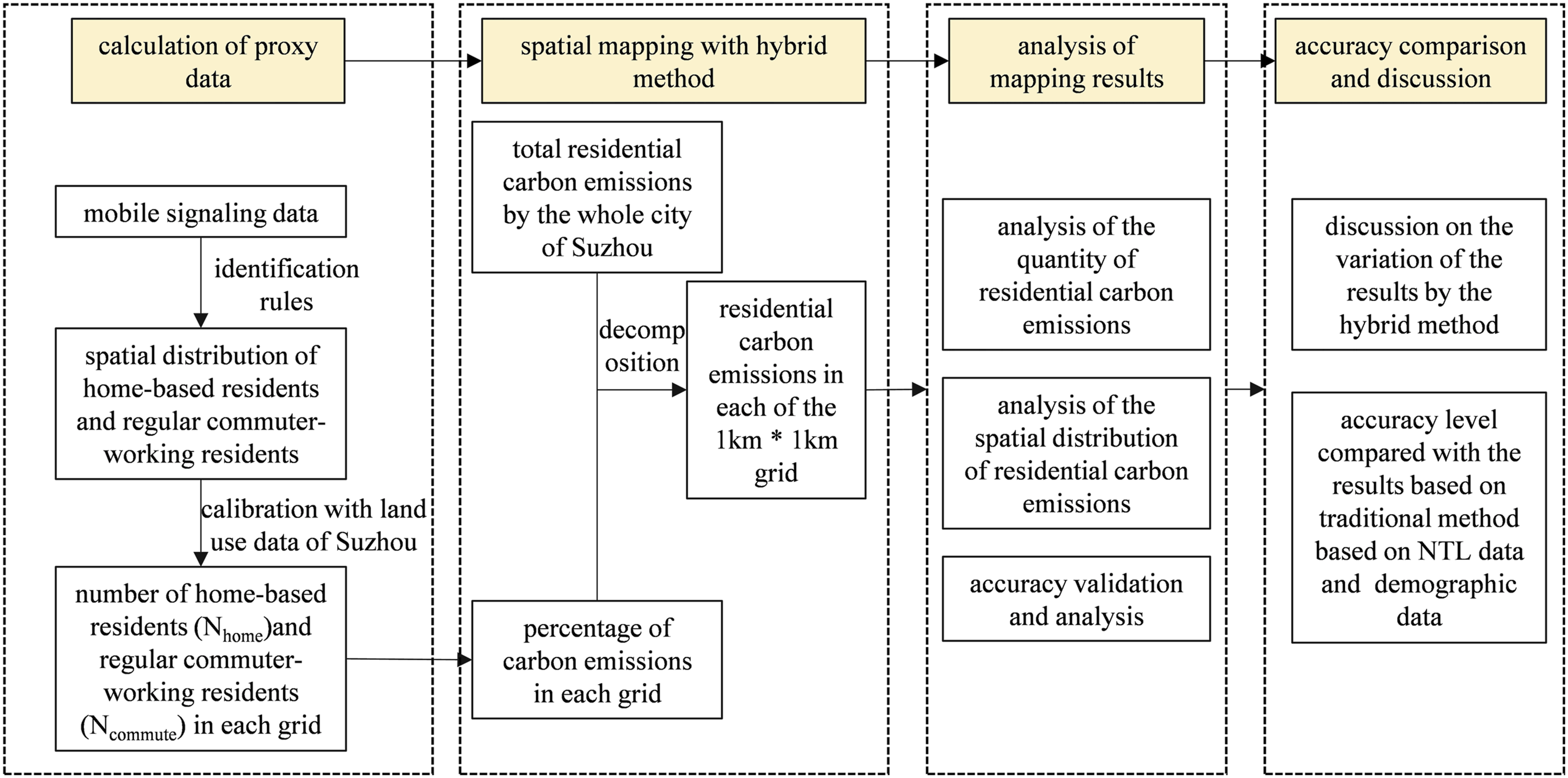

The emission data of all grids were then visualised in ArcGIS, which generated a residential carbon emission map of Suzhou with a spatial resolution of 1 km × 1 km. Based on the mapping results, the quantity and spatial distribution of residential carbon emissions in Suzhou were analysed. Additionally, to justify accuracy, the total amount of residential carbon emissions from each municipal district and/or county was calculated by combining the residential carbon emissions from all grids within each administrative district. The resulting emissions figure in each administrative district was then checked against the data, as stated in the Statistical Yearbook of Suzhou (2020), to determine the difference between the two.

To highlight the merits of the hybrid modelling method, we used demographic and NTL data as proxy data to map the residential carbon emissions of Suzhou. The mapped results based on these two conventional methods were compared with the results of the hybrid approach. One dimension was to ascertain which of the three results was closer to the data, as stated officially in the Statistical Yearbook, and the other was to ascertain which method can produce a more stable estimation (i.e. closeness to the real data with less variance).

The hybrid mapping model

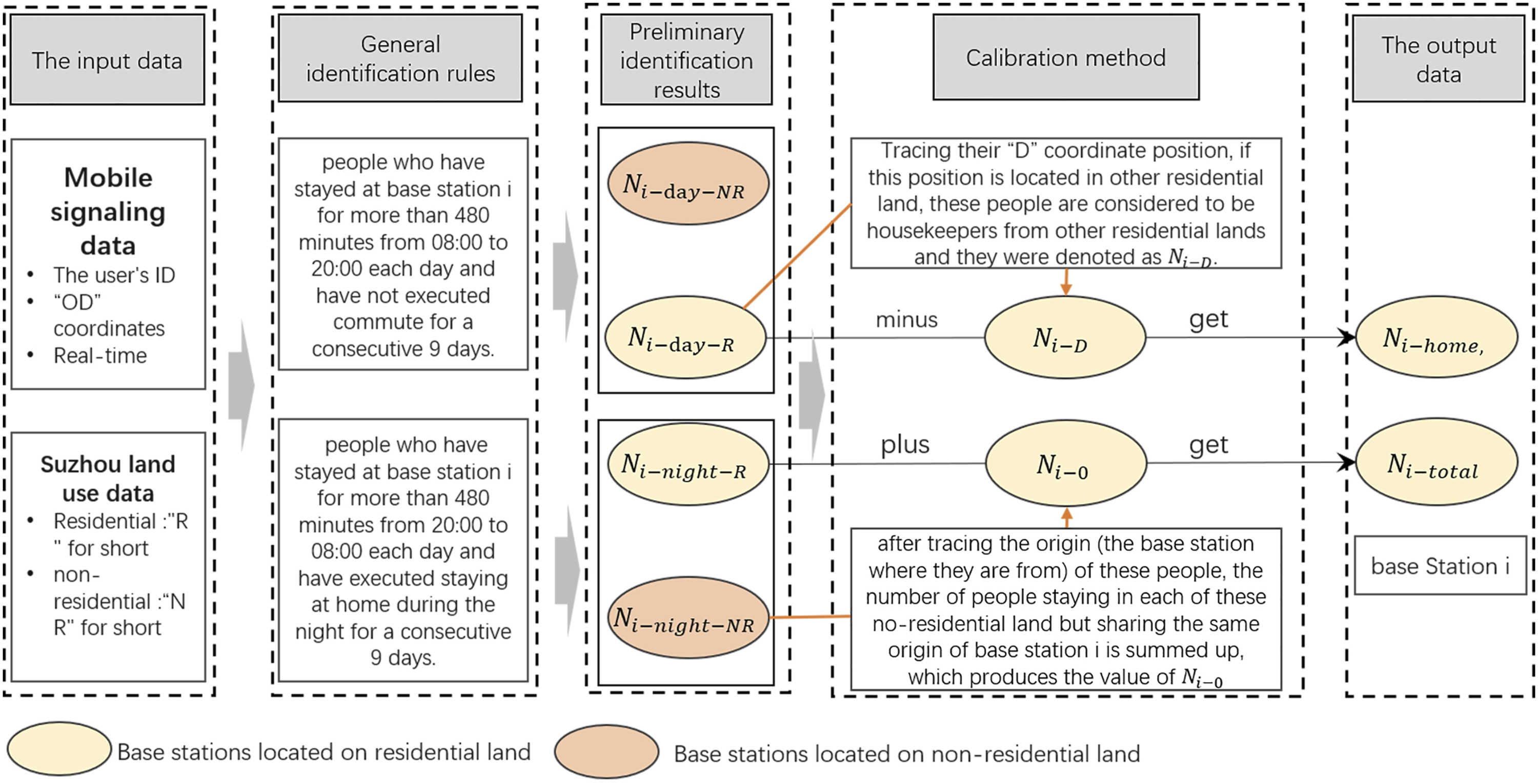
Identification of the home-based residents and regular commuter-working residents

To facilitate the explanation of the identification method (Figure 2), it was assumed that we were dealing with the identification and differentiation of home-based and regular commuter-working residents recorded by a base station located on residential land. Generally, by using mobile signalling data covering the timespan from 08:00 to 20:00, we can directly acquire the total population recorded by base station i during daylight, denoted as $N_{i - d a y - R}$ . However, considering that there are many housekeepers from other residential lands (origin) who are employed by householders to work on residential land within the coverage of base station i (destination) during the day, the number of home-based residents (denoted as $N_{i - h o m e}$ ) should be $N_{i - d a y - R}$ - $N_{i - D}$ rather than $N_{i - d a y - R}$ , where $N_{i - D}$ represents the number of housekeepers working on that residential land in daylight (Formula (1)). Similarly, using mobile signalling data covering the timespan from 20:00 to 08:00, we can directly acquire the population recorded by base station i during the night, denoted as $N_{i - n i g h t - R}$ . Again, $N_{i - n i g h t - R}$ cannot be used to represent the real total number of residents living on residential land where base station i is located because some residents from this residential land work the night shift on other lands. If we denote the number of residents who work night shifts on residential land within the coverage of base station i as $N_{i - t o t a l}$ , this should be equal to $N_{i - n i g h t - R}$ + $N_{i - O}$ (Formula (2)). With these data, the number of regular commuter-working residents on residential land within the coverage area of base station i (denoted as $N_{i - c o m m u t e}$ ) should be equal to $N_{i - t o t a l}$ - $N_{i - h o m e}$ (Formula (3)). Finally, we obtained the real $N_{i - c o m m u t e}$ , $N_{i - h o m e}$ , and $N_{i - t o t a l}$ for the residential land covered by base station i as follows

N_{i - h o m e} = N_{i - d a y - R} - N_{i - D}

(1)

N_{i - t o t a l} = N_{i - n i g h t - R} + N_{i - O}

(2)

N_{i - c o m m u t e} = N_{i - t o t a l} - N_{i - h o m e}

(3)

In Formula (1),

N_{i - d a y - R}

represents the total number of people who have stayed on residential land within the coverage area of base station i for more than 480 min from 08:00 to 20:00 each day and have not commuted for nine consecutive days.

N_{i - D}

denotes the number of people who have stayed on residential land within the coverage of base station i for more than 480 min from 08:00 to 20:00 but have commuted for nine consecutive days, which can be identified by tracing the origins of their travel using mobile signalling data. In Formula (2),

N_{i - n i g h t - R}

denotes the number of people who stayed on residential land within the coverage of base station i for more than 480 min from 20:00 to 08:00 each day and stayed at home during the night for nine consecutive days.

N_{i - O}

represents the number of residents who should have stayed on residential land within the coverage of base station I, but not because of their work on the night shift in other land plots. First, the people who stayed in each of the non-residential lands during the night (20:00–08:00) were identified. Then, after tracing the origin of these people (the base station from which they are from), the number of people staying in each of these non-residential lands but sharing the same origin as base station i was summed up, which produced the value of

N_{i - O}

Figure 2.

Identification and calibration methods.

By combining the number of identified populations in each of the residential grids contained in each administrative district, we acquired the total identified population of each administrative district, as shown in Table 2. The total population of Suzhou, as stated in the Statistical Yearbook is approximately 10.75 million. In contrast, the identified total population was approximately 7.57 million, accounting for 70.4% of the total population. The number of identified regular commuter-working residents was 5.44 million, accounting for 71.8% of the identified total population. Moreover, for each administrative district, the ratio of identified regular commuter-working residents to the total identified population of Suzhou was close to that of the employed population to the total population of Suzhou, according to the Statistical Yearbook. For example, the identified regular commuter-working residents in the urban areas took up 51.87% of the total number of the identified regular commuter-working residents in Suzhou. In contrast, the percentage of the employed population to the total employed population, as presented in the Statistical Yearbook is 50.27%. Generally, the difference between the identified data and officially stated data in percentage was extremely low in Taicang, Wujiang, and Zhangjiagang, whereas in the urban area and Kunshan, this difference was slightly higher. The insignificance of this nuance implied that the data identified using the hybrid method were highly representative and credible.

Table 2.

Comparison between the identified population and the population from statistical book.

Groups		Identified total population	Number of identified regular commuter-working residents	Total population by statistical yearbook	Employed population by statistical yearbook
Inner urban area	Total	378.83	251.08	557.6	348.2
Inner urban area	Percentage	50.04%	51.87%	46.19%	50.27%
Inner urban area (Wujiang)	Total	95.58	72.24	131.26	86.16
Inner urban area (Wujiang)	Percentage	12.63%	12.21%	13.29%	12.44%
Changshu	Total	96.69	75.35	151.89	104.38
Changshu	Percentage	12.77%	14.13%	13.86%	15.07%
Zhangjiagang	Total	77.33	62.2	126.4	77.1
Zhangjiagang	Percentage	10.21%	11.76%	11.44%	11.13%
Kunshan	Total	154.13	107.78	166.92	117.11
Kunshan	Percentage	20.36%	15.53%	21.66%	16.91%
Taicang	Total	50.09	37.21	72.12	45.81
Taicang	Percentage	6.62%	6.71%	6.84%	6.61%

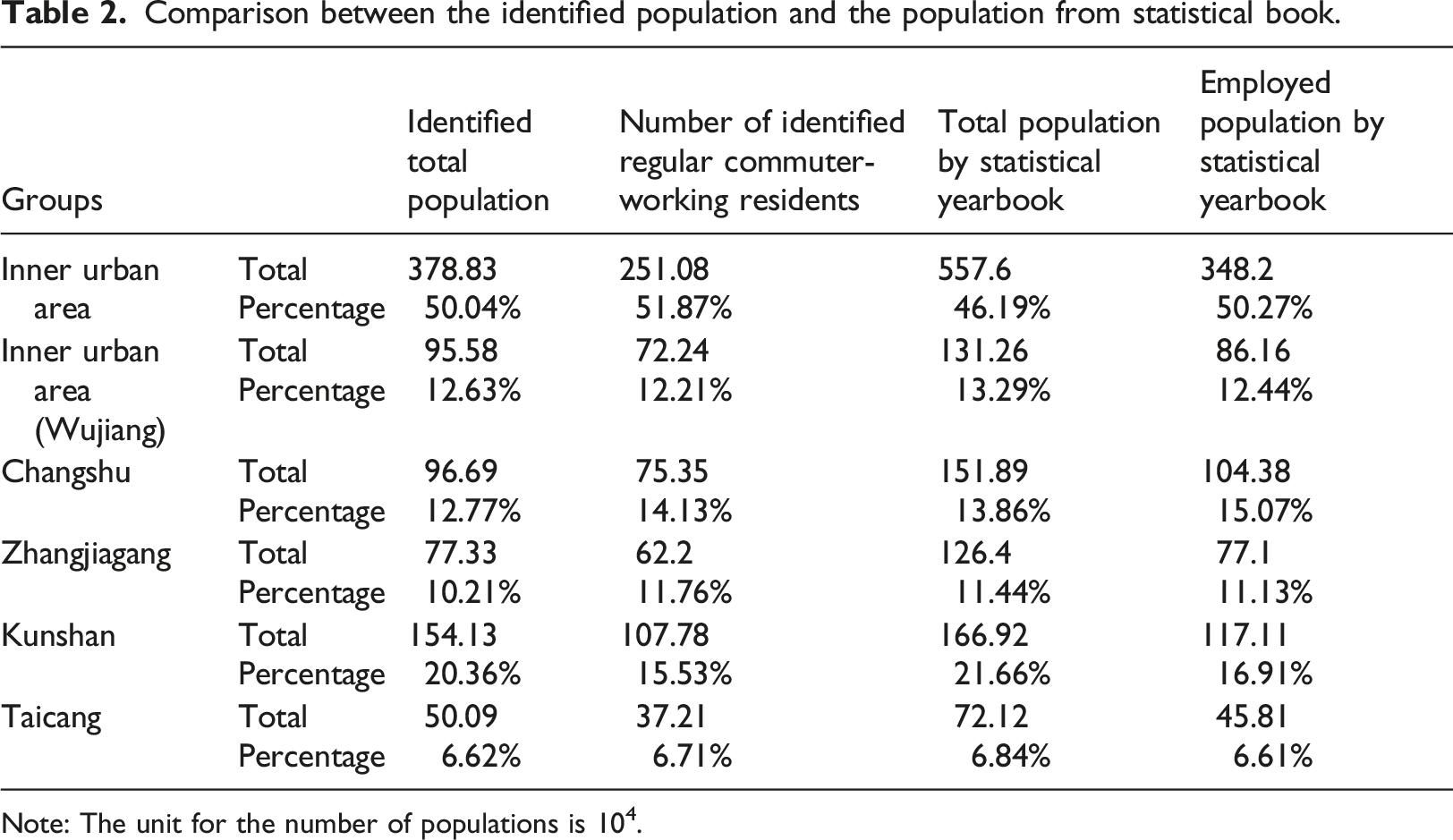
Note: The unit for the number of populations is 10⁴.

Calculation and mapping of the residential carbon emissions

To achieve a high-spatial-resolution simulation, the entire city of Suzhou was first gridded with a spatial resolution of 1 km × 1 km using ArcGIS. Then, by overlap analysis, the grids subject to or containing residential land-use plots were identified, through which 2186 grids were selected as the statistical units. Then, $N_{j - c o m m u t e}$ , $N_{j - h o m e}$ , and $N_{j - t o t a l}$ in grid j were obtained by summarising the calibration population data ( $N_{i - c o m m u t e}$ , $N_{i - h o m e}$ , and $N_{i - t o t a l}$ ) recorded by the base station located in the grid.

In this study, it was assumed that the time spent at home by home-based residents is 24 h and that spent by regular commuter-working residents is 12 h. Therefore, the total hours spent by residents consuming energy at home in grid j ( $w_{j}$ ) can be calculated using equation (4)

w_{j} = N_{j - c o m m u t e} * 12 + N_{j - h o m e} * 24

(4)

Assuming that each resident consumes the same amount of energy per hour, the total residential carbon emissions in grid j ( $C_{j}$ ) can be calculated using equation (5)

C_{j} = \frac{w_{j}}{\sum w_{j}} \cdot C_{P} \cdot μ

(5)

where

C_{P}

is the total household electricity consumption of Suzhou and

μ

is the carbon emissions factor of electricity as stated by IPCC (

μ = 0.785

Results

Estimation accuracy level

To justify the estimation accuracy of the proposed hybrid method, we propose the statistic $H_{k}$ which can be calculated using Formula (6)

H_{k} = (1 - \frac{| Σ C_{k j} - C_{k p} |}{C_{k p}}) \cdot 100 %

(6)

where

H_{k}

is the proximity level;

C_{k j}

is the residential carbon emissions by grid j in administrative district k, which can be calculated by Formula (5);

Σ C_{k j}

is the sum of the residential carbon emissions from all the grids in administrative district k; and

C_{k p}

is the total residential carbon emissions of administrative district k, which is stated in the Statistical Yearbook.

As illustrated in Figure S2 in the Supplementary Material, the estimated results show that urban areas have the highest residential carbon emissions, reaching 5548.10 kt annually, followed by Kunshan. In contrast, Taichang had the lowest annual residential carbon emissions, with annual emission of 689.83 kt. Regarding the accuracy of the estimation, each of the six administrative districts had percentages higher than 93%. Changshu had the highest accuracy level at 98.22%, implying that the hybrid mapping model as proposed in this study is highly reliable.

Total residential carbon emissions

The mapping results show that residential carbon emissions from inner urban areas accounted for more than half of the total emissions in Suzhou. More importantly, approximately 39.56% of the residential carbon emissions are contributed by the centre-most area of Suzhou (the inner urban area without Wujiang district), where high a density of human activities occurs. In contrast, Taicang and Zhangjiagang contributed the lowest percentage of residential carbon emissions to the total emissions of the city.

Regarding the quantitative distribution feature, and by taking the residential grid as the statistical unit, the Pareto plot of the residential carbon emissions revealed that for the entire city of Suzhou, 30.92% of the residential sites have contributed 80% of the total residential carbon emissions. However, as shown in Figure S3 in the Supplementary Material, there were variations among the six administrative districts. Changshu and Taicang had the lowest percentages at 18.94% and 21.31%, respectively, which closely conforms to the Pareto principle. In contrast, the remaining districts, including the inner urban area, Wujiang, Zhangjiagang, and Kunshan, had a percentage higher than 30%, with Zhangjiagang having the highest. This means that residential carbon emissions are more evenly distributed in these districts than in Changshu and Taicang.

Spatial distribution of residential carbon emissions

Figure 3 illustrates the mapping results for residential carbon emissions. Each of the six administrative districts had a clustered area with high residential carbon emissions. Generally, these clustered areas are the centres of the districts. However, Kunshan and the inner urban areas displayed distinctiveness. For example, the spatial distribution of residential carbon emissions in Kunshan has shown residential carbon emission corridors extending from the centre of Kunshan towards the metropolitan area of Shanghai, located to the southeast. Additionally, it has also formed an emissions corridor connected to the core urban area (as shown encircled by the red line in Figure 3), which accounts for approximately 60% of the residential carbon emissions of Suzhou. This coincides with the fact that numerous residential buildings are occupied by a large number of citizens along traffic arteries between the core urban area and centre of Kunshan.

Figure 3.

The mapping results of 1 km * 1 km resolution residential carbon emission (unit: kt).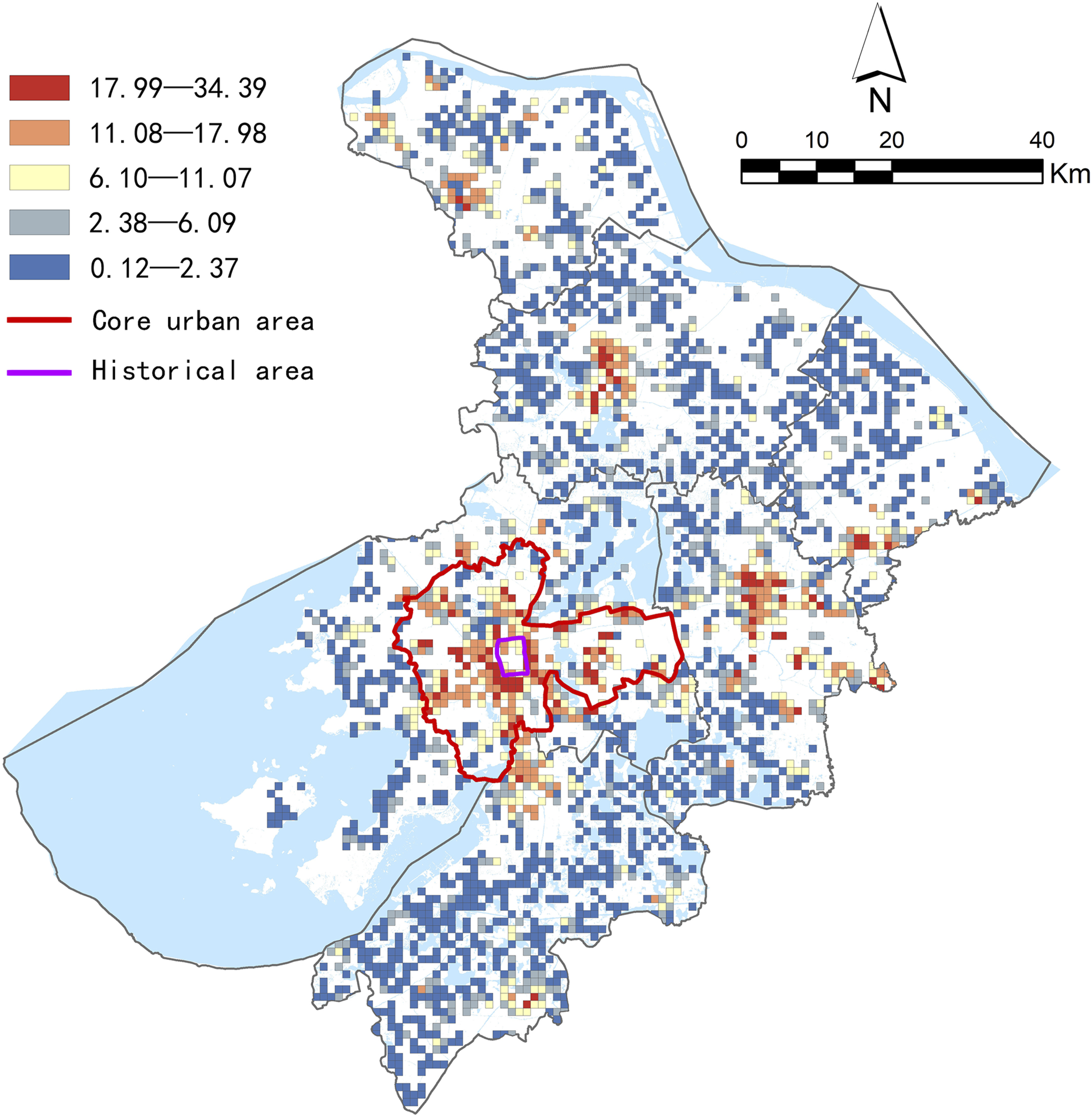

In inner urban areas, sites with high residential carbon emissions also showed a clustering pattern. In contrast to the other districts, these sites of high emissions are not collocated within a small area but dispersed within the core urban area. Notably, it displays a low-high-low pattern from the core to the outside. Additionally, it featured a radiative pattern with some high-emission corridors extending from the historical area towards its fringe. It is worth noting that the low emission density site is located in the old historical urban area (encircled by the purple line). The sites of high-density emissions come close to the historical urban area, with some residential grids in particular featuring the highest density located near its south. This outcome aligns with the fact that the old historical urban area is being strictly preserved and housing around it is being favoured by citizens, particularly the rising middle class (He and Liu, 2010).

Discussion

Nuance between the estimated values and those from the Statistical Yearbook

Despite the high proximity level of the estimated values to the data from the official Statistical Yearbook, there is still a need for further exploration. The largest difference in the official values and the estimated values is approximately 6%. One cause for this nuance could be the supposition that all residents in Suzhou share the same amount of energy consumption per capita. In a general sense, it is very likely that people with higher incomes have a higher level of per capita energy consumption at home and, thus, a higher level of per capita residential carbon emissions. This might explain why the estimated residential carbon emissions in the inner urban area were slightly lower than the values from the Statistical Yearbook. In general, the average income of residents in the inner urban area was higher than that in other districts. Therefore, the average per capita energy consumption was higher in the inner urban areas. However, the estimation assumes the same per capita energy consumption, which will assuredly lead to underestimation of residential carbon emissions in the inner urban area.

It is also possible that the total population in the residential grids was overestimated using mobile signalling data, which could consequently lead to an overestimation of the total amount of residential carbon emissions. In practice, industrial grids may surround residential grids. In this circumstance, if the mobile phone base station is located precisely in these grids, then those workers in the industrial grids could be counted as residents subject to the residential grids, which in certain cases will lead to an overestimation of residential carbon emissions. As these possibilities are commonly observed in Kunshan, Zhangjiagang, and Taicang, the estimated values for these three districts are slightly higher than those shown in the Statistical Yearbook.

The supposition that the time spent at home by regular commuter-working residents at home is 12 h and that of home-based residents is 24 h could also lead to this nuance. To justify this point, the time spent by regular commuter-working residents was taken as an example for further analysis, when the time spent by home-based residents at home was still supposed to be 24 h. We re-estimated the residential carbon emissions of each grid by changing the assumed time to 6 h, 7 h, 8 h, 9 h, 10 h, 11 h, and 13 h. The results show that with the supposition of 7 h, the estimated values for almost all six administrative districts, reached the highest accuracy level with the highest average proximity level, 98.38%. In particular, the proximity level for Changshu reached 99.80% (Table S1 in the Supplementary Material). Although this result does not appear reasonable, as 7 h of home time is very small, it is enough to show how much overtime Chinese people work and how busy their lives really are.

Advantages of the hybrid modelling method

To justify the advantage of the proposed hybrid modelling method over conventional approaches, we estimated residential carbon emissions using NTL data (denoted method A) and the identified total population as proxy data (denoted method B). By referring to previous studies (Zhuo et al., 2015), grids (1 km × 1 km) with a proportion of residential land-use greater than 50% were identified as residential grids. It was found that 1398 grids were residential grids. Regarding Method A, the residential carbon emissions of each of the identified residential grids were calculated using Formula (5), treating $w_{i}$ as the brightness of the grid. For Method B, Formula (5) was also used, but the value of $w_{i}$ was the size of the identified population represented by $N_{i - t o t a l}$ in Formula (2). It is worth noting that the size of the identified population was calibrated by considering residents on the night shift, which partially improved the estimation accuracy.

With the estimated residential carbon emissions, it was possible to calculate the proximity levels of both method for each of the six administrative districts. As illustrated in Figure S4 in the Supplementary Material, the average proximity level of Method A was 85.54%, with 67.82% as the lowest level and 96.64% as the highest. In contrast, the highest proximity level for Method B was 93.98%, whereas the lowest was 91.26%. This implies that, generally, the accuracy level of the modelling method, considering the size of the identified population as proxy data, is higher than that using NTL as proxy data. In particular, neither Method A nor Method B have an accuracy level higher than that of the hybrid modelling method, which takes the total time at home as proxy data. Moreover, considering the deviation in the proximity level, the hybrid method has the lowest deviation, whereas Method B has a slightly higher deviation, and Method A has a much higher deviation. This indicates that the estimation of residential carbon emissions based on the hybrid method was more stable and reliable.

Conclusions

In this study, we propose a hybrid modelling method to map urban residential carbon emissions with a spatial resolution of 1 km × 1 km using multi-source data. The central idea is to use the total time spent at home by residents as proxy data rather than the number of identified residents or the brightness of the grid based on NTL data, which are commonly adopted in conventional modelling approaches. Therefore, a clear identification of regular commuter-working residents and home-based residents is key because their time spent at home differs. To do this, we used land-use data in conjunction with mobile signalling data to identify the residents on night shifts and those possibly working as housekeepers during the day. With these data, it was possible to calculate the number of home-based residents and regular commuter-working residents in each 1 km × 1 km residential grid.

Assuming that home-based residents spend 24 h at home and regular commuter-working residents spend 12 h at home, we produced a high-spatial resolution map of the urban residential carbon emissions of Suzhou. The results show that more than half of the residential carbon emissions originated from the inner urban area (core urban area plus Wujiang). Additionally, residential carbon emissions were roughly clustered at the centre of each of the six districts. In contrast to the other districts, residential carbon emissions in the inner urban area displayed a low-high-low spatial pattern from the centre towards the fringe, with some high-emission corridors extending outwards from the historical area.

By comparing the estimated results with the data stated in the official Statistical Yearbook, the average proximity level is greater than 96.37%, which implies that estimation of the residential carbon emissions based on the hybrid method is highly accurate. It is worth noting that the results would be more accurate if there were real statistics for a certain number of grids to be verified. It was also found that by the hybrid method, the average proximity level can reach up to 98.38% if we assume that the regular commuter-working resident spends 7 h at home. To justify the advantage of the hybrid method, we also calculated the proximity level of the method using the size of the identified population as the proxy data and the brightness based on the NTL data as proxy data. It was revealed that the estimated results based on the hybrid approach had the highest accuracy and lowest deviation, whereas the performance of the method based on NTL data was the worst.

In this study, high-resolution spatial mapping of residential carbon emissions was obtained using a hybrid approach of 1 km × 1 km grids, which helped achieve high-resolution spatial mapping of citywide sectoral carbon emissions. This is important for gaining understanding of the complex socio-ecological system and implementing sectoral and space-based strategies for carbon mitigation (Duit et al., 2010). The hybrid modelling method can also be used to map residential carbon emissions by sector, such as transport and commercial activities. However, this hybrid approach cannot be executed or applied to other cases without the availability of long-term (at least 1 week) mobile signalling data and detailed land-use data. Additionally, if we can acquire detailed data on the energy consumed by each residential district/household, then there is no need to use this approach, and the residential carbon emissions from each residential grid can be easily calculated. However, in practice, this type of data cannot be easily acquired because of privacy protection issues. Therefore, the hybrid approach proposed here is still a viable choice, as it not only overcomes the privacy issue but also has prominent performance in terms of estimation accuracy and stability.

Supplemental Material

Supplemental Material - Hybrid method of mapping urban residential carbon emissions with high-spatial resolution: A case study of Suzhou, China

Supplemental Material for Hybrid method of mapping urban residential carbon emissions with high-spatial resolution: A case study of Suzhou, China by Junyang Gao, Helin Liu, Yongwei Tang and Mei Luo in Environment and Planning B: Urban Analytics and City Science

Footnotes

Declaration of conflicting interests

The author(s) declared no potential conflicts of interest with respect to the research, authorship, and/or publication of this article.

Funding

The author(s) disclosed receipt of the following financial support for the research, authorship, and/or publication of this article: This work was supported by The Natural Science Foundation of Hubei Province; 2021CFB012, National Natural Science Foundation of China; 52278063, 41901390.

ORCID iD

Helin Liu

Supplemental Material

Supplemental material for this article is available online.

Junyang Gao is currently a doctoral student of the School of Architecture and Urban Planning of Huazhong University of Science and Technology. His research interests are in low carbon spatial planning, and computational modelling of urban and regional planning based on big data. He holds degrees from Huazhong University of Science and Technology (BEc. and MEc.). Email: jy425@hust.edu.cn. Postal address: South Building 2, No.1037 Luoyu Road, Hongshan District, Wuhan, Hubei Province, China. (430074).

Helin Liu is currently professor of planning and is working in the School of Architecture and Urban Planning, Huazhong University of Science and Technology, China. His research interests are in computational modelling of urban and regional planning based on big data and artificial intelligence, climate change mitigation and adaptive planning. He holds degrees from Nanjing University (BSc. and MSc.) and the University of Cambridge (Ph. D).Academic title: Professor. Email: hl362@hust.edu.cn. Phone: +86 15527719130. Postal address: Room309, South Building 2, No.1037 Luoyu Road, Hongshan District, Wuhan, Hubei Province, China. (430074).

Yongwei Tang is currently a doctoral student of the School of Architecture and Urban Planning of Huazhong University of Science and Technology, and a registered urban and rural planner. His research interests are in urban and rural planning and design decision-making based on data support, focusing on urban spatial structure research, innovation economy, and urban spatial planning strategies. He holds degrees from Lanzhou University (BSc. and MSc.). Email: D202181219@hust.edu.cn. Postal address: South Building 2, No.1037 Luoyu Road, Hongshan District, Wuhan, Hubei Province, China. (430074).

Mei Luo is currently a doctoral student of the School of Architecture and Urban Planning of Huazhong University of Science and Technology, and a student of Hubei Engineering Technology Center and the key Laboratory of Urban Simulation for Ministry of natural resources. Her research interests are in low carbon spatial planning, and regional planning. She holds degrees from Huazhong agricultural university (BSc. and MSc). Email: D202081117@hust.edu.cn. Postal address: South Building 2, No.1037 Luoyu Road, Hongshan District, Wuhan, Hubei Province, China. (430074).

References

Bai

Dawson

Ürge-Vorsatz

, et al. (2018) Six research priorities for cities and climate change. Nature Publishing Group 55: 23–25.

Cai

Dhakal

, et al. (2018a) Source data supported high resolution carbon emissions inventory for urban areas of the Beijing-Tianjin-Hebei region: spatial patterns, decomposition and policy implications. Journal of Environmental Management 206: 786–799.

Cai

Liang

Zhou

, et al. (2018b) China high resolution emission database (CHRED) with point emission sources, gridded emission data, and supplementary socioeconomic data. Resources, Conservation and Recycling 129: 232–239.

Cai

Shi

Ren

, et al. (2021) The need for urban form data in spatial modeling of urban carbon emissions in China: a critical review. Journal of Cleaner Production 319: 128792.

Cai

Shi

Ren

(2020) Developing a high-resolution emission inventory tool for low-carbon city management using hybrid method-A pilot test in high-density Hong Kong. Energy and Buildings 226: 110376.

Duit

Galaz

Eckerberg

, et al. (2010) Governance, complexity, and resilience. Global Environmental Change 20: 363–368.

Gong

Chen

, et al. (2020) Mapping essential urban land use categories in China (EULUC-China): preliminary results for 2018. Science Bulletin 65: 182–187.

Liu

(2010) Mechanism and consequences of china’s gentrification under market transition. Geographic Science 30: 496–502.

IPCC (2014) IPCC, 2014: climate change 2014: synthesis report. In: Contribution of Working Groups I II and III to the Fifth Assessment Report of the Intergovernmental Panel on Climate Change. Geneva, Switzerland, Jun: IPCC.

10.

Jing

Bai

Luo

, et al. (2018) A top-bottom method for city-scale energy-related CO2 emissions estimation: a case study of 41 Chinese cities. Journal of Cleaner Production 202: 444–455.

11.

Lai

Chen

, et al. (2022) Exploring employment spatial structure based on mobile phone signaling data: the case of Shenzhen, China. Land 7(11): 983–997.

12.

Meng

Graus

Worrell

, et al. (2014) Estimating CO2 (carbon dioxide) emissions at urban scales by DMSP/OLS (defense meteorological satellite program’s operational linescan system) nighttime light imagery: methodological challenges and a case study for China. Energy 71: 468–478.

13.

Sharifi

Khamchiangta

, et al. (2018) Urban carbon mapping: towards a standardized framework. Energy Procedia 152: 799–808.

14.

Shi

Chen

, et al. (2016) Modeling spatiotemporal CO2 (carbon dioxide) emission dynamics in China from DMSP-OLS nighttime stable light data using panel data analysis. Applied Energy 168: 523–533.

15.

Sharifi

Yang

, et al. (2018) Mapping building carbon emissions within local climate zones in Shanghai. Energy Procedia 152: 815–822.

16.

Zhang

Fang

Zhou

, et al. (2020) Measuring megaregional structure in the Pearl River Delta by mobile phone signaling data: A complex network approach. Cities c(104): 102809–102820.

17.

Zhuo

Zheng

Zhang

, et al. (2015) An improved method of night-time light saturation reduction based on EVI. International Journal of Remote Sensing 36: 4114–4130.

Supplementary Material

Please find the following supplemental material available below.

For Open Access articles published under a Creative Commons License, all supplemental material carries the same license as the article it is associated with.

For non-Open Access articles published, all supplemental material carries a non-exclusive license, and permission requests for re-use of supplemental material or any part of supplemental material shall be sent directly to the copyright owner as specified in the copyright notice associated with the article.

0.00 MB

0.83 MB

Hybrid method of mapping urban residential carbon emissions with high-spatial resolution: A case study of Suzhou,China

Abstract

Keywords

Introduction

Materials and methods

Study area and data

Research framework

The hybrid mapping model

Identification of the home-based residents and regular commuter-working residents

Calculation and mapping of the residential carbon emissions

Results

Estimation accuracy level

Total residential carbon emissions

Spatial distribution of residential carbon emissions

Discussion

Nuance between the estimated values and those from the Statistical Yearbook

Advantages of the hybrid modelling method

Conclusions

Supplemental Material

Supplemental Material - Hybrid method of mapping urban residential carbon emissions with high-spatial resolution: A case study of Suzhou, China

Footnotes

Declaration of conflicting interests

Funding

ORCID iD

Supplemental Material

References

Supplementary Material