Sage Journals: Discover world-class research

Abstract

Identifying market segments can improve the fit and performance of hedonic price models. In this paper, we present a novel approach to market segmentation based on the use of machine learning techniques. Concretely, we propose a two-stage process. In the first stage, classification trees with interactive basis functions are used to identify non-orthogonal and non-linear submarket boundaries. The market segments that result are then introduced in a spatial econometric model to obtain hedonic estimates of the implicit prices of interest. The proposed approach is illustrated with a reproducible example of three major Spanish real estate markets. We conclude that identifying market sub-segments using the approach proposed is a relatively simple and demonstrate the potential of the proposed modelling strategy to produce better models and more accurate predictions.

Keywords

Hedonic prices market segments decision trees spatial econometrics reproducible research

Introduction

Hedonic price analysis is one of the most widely-used approaches for the study and valuation of properties in real estate markets. This approach is attractive due to its strong theoretical grounding and appealing interpretation (Rosen, 1974). Indeed, when hedonic price models are estimated using multiple linear regression the coefficients of the model are thought to capture the implicit prices of attributes in a bundled good. In this way, while a room may lack an explicit price in the valuation of a property, the coefficient of a hedonic price model quantifies its implicit value. Such decomposition of the price of a bundled good into the implicit prices of its constituent parts is important for multiple reasons: this analysis is the industry standard for property assessment for tax purposes (Morillo et al., 2017); these models are used to quantify the willingness to pay for non-market environmental amenities (Montero et al., 2018), including air quality and open spaces and similarly they can be used to assess the cost of disamenities (e.g., Von Graevenitz, 2018).

The need to assess property values in a transparent, accurate, and precise way has led to numerous developments. A strand of research has aimed at enhancing the performance of models by incorporating spatial information. Geographic Information Systems (GIS) in particular have been used to make explicit some attributes of properties and their environments that might otherwise be overlooked (Paterson and Boyle, 2002). The use of spatial data, in turn, has brought increased attention to the question of statistical sufficiency and therefore the need for approaches that appropriately consider the issues of spatial association and spatial heterogeneity in hedonic price analysis (Pace and Gilley, 1997; Paez et al., 2001). As a result, there has been a proliferation of studies that apply spatial statistical or econometric methods to the issue of property valuation (Paez, 2009). Recent applications include the use of hierarchical spatial autoregressive models (Cellmer et al., 2019), moving windows approaches (Páez et al., 2008), spatial filtering (Helbich and Griffith, 2016), and kriging techniques (Montero-Lorenzo et al., 2009), among others.

In addition to interest in spatial data, the application of machine learning techniques for hedonic price analysis has also become an active topic of research. There are at least two distinct ways in which machine learning can be used for hedonic price analysis. In some studies, the role of machine learning algorithms is to process information that would otherwise be difficult or impossible to obtain using non-automated means. The information obtained is then used as an input in econometric hedonic models. For example, Humphreys et al. (2019) and Nowak and Sayago-Gomez (2018) used machine learning classifiers to ethnically profile buyers and sellers based on last names to understand whether potential cultural biases and/or discrimination issues exist in property transactions. In other research, machine learning algorithms replace the conventional hedonic price model (Hu et al., 2019; Yoo et al., 2012; Füss and Koller, 2016). The evidence available shows that machine learning methods can perform remarkably well, but can also be seen as black boxes with low interpretability (see James et al., 2013).

Our objective in this paper is to introduce a novel approach that retains the interpretability of econometric approaches, but is enhanced by the identification of spatial market segments obtained from the use of machine learning techniques. We propose a two-stage approach. In the first stage, classification trees are implemented to identify homogeneous spatial market segments. The number of market segments is endogenous, and, compared to Füss and Koller (2016), the use of interactive basis functions (see Paez et al., 2019) can accommodate non-orthogonal and non-linear decision boundaries. The market segments are then introduced as covariates in an econometric model. This approach can potentially enhance the model without compromising its interpretability.

A reproducible case study of property values in three major markets in Spain helps to illustrate the proposed approach. Following recommendations for openness and reproducibility in geospatial research (Paez, 2021), this paper is accompanied by a fully documented and open data product (see Arribas-Bel et al., 2021), and the code is embedded in a self-contained R markdown document. The results show that modeling prices using the approach proposed to identify spatial market segments improves the fit of the models and can in addition enhance the quality of predictions.

Spatial market segmentation

The importance of housing submarkets has long been recognized in the literature (e.g., Rapkin et al., 1953). Market differentiation can be the result of a variety of processes operating separately or in conjunction, including substitution, differentiation, and variations in consumer preferences (Galster, 1996). In principle, this implies a degree of homogeneity within the market segment that differentiates it from other segments. According to (Thibodeau, 2003, pp. 4–5) a spatial housing submarket “defines a geographic area where the price of housing per unit of housing service is constant.” Given the non-tradeable nature of location, research has shown the relevance of spatial market segments (Bourassa et al., 2007; Royuela and Duque, 2013; Usman et al., 2020).

Submarket analysis is often implemented in a pragmatic way, encompassing regional boundaries, for instance those of metropolitan regions, cities, or municipalities. It has long been recognized, though, that submarkets may exist at smaller scales (e.g., Rapkin et al., 1953). In particular, the pioneering work of Alonso (Alonso, 1964) on urban structure led to the realization of the importance of geography in terms of differentiation of real estate property. Since then, vast amounts of empirical evidence have contributed to demonstrate just how commonplace differences in hedonic prices are at the intraurban scale. Concurrently, market segmentation has been shown to be not only a conceptually sound practice (see Watkins, 2001), but also conducive to higher quality models and improved predictive performance, in particular when geography is explicitly taken into consideration (Páez et al., 2008).

Numerous approaches have been proposed to identify market segments. Some are based on expert opinion, such as from appraisers (Wheeler et al., 2014). Many others are data-driven, using statistical or machine learning techniques (e.g., Helbich et al., 2013; Wu et al., 2018). Heuristic approaches also exist that exploit the latent homogeneity in values (Royuela and Duque, 2013). Implementation of market segments in hedonic price models can be accomplished by means of fixed effects (i.e., dummy variables) for sub-regions (e.g., Bourassa et al., 2007), spatial drift by means of a trend surface (e.g., Pace and Gilley, 1997), spatially autoregressive models (e.g., Pace et al., 1998), switching regressions (e.g., Islam and Asami, 2011; Paez et al., 2001), multilevel and/or Bayesian models (e.g., Wheeler et al., 2014), or by means of spatially moving windows or non-parametric techniques to obtain soft market segments (Páez et al., 2008; Hwang and Thill, 2009). As is commonly the case, there is no one technique that performs consistently better than the alternatives in every case, since performance depends to some extent on the characteristics of the process being modeled (Usman et al., 2020). It is therefore valuable to explore alternative approaches to identify and model market segments, to further enrich the repertoire of techniques available to analysts.

A recent proposal along these lines is due to Füss and Koller (2016), who suggest using decision trees to identify and model market segments. James et al. (2013) list some attractive features of decision trees. They are relatively simple to estimate and intuitive to interpret. They divide attribute space into a set of mutually exclusive and collectively exhaustive regions, and thus are ideally suited for market segmentation. By design, the regions generated are spatially compact and internally homogeneous. And they can outperform other regression techniques. Market segments derived from a decision tree can be used in combination with other modeling techniques, such as a second-stage tree regression (with fixed effects for the market segments from the preliminary tree regression), linear models, or models with spatial or spatio-temporal effects, such as space-time autoregression. Füss and Koller (2016) compare several different modeling techniques. Their findings confirm that introducing a form of market segmentation greatly improves prediction accuracy, and the use of tree-based market segments does so more than the use of an a priori zoning system defined by ZIP codes. Furthermore, accounting for residual spatial pattern in the form of a spatial autoregressive model further improves the accuracy of estimation.

The results reported by Füss and Koller (2016) are appealing. However, the modeling strategy that they implement inherits a limitation of tree regression, namely, the relatively inflexible way in which attribute space is partitioned using recursive binary splits. What this means is that market segments obtained in this way are limited to rectangular shapes (see page 1359 in Füss and Koller, 2016). While prediction accuracy reportedly improves with tree-based segmentation of the market, it might be desirable to define market segments more flexibly so that they are not constrained to rectangular shapes. Second, estimates of a regression tree are the mean of the values contained in the volume of a leaf, which means they are constants for each leaf. In a geographical application, the leaves are mutually exclusive and collectively exhaustive partitions of geographical space. Using the residuals in the second step of the modelling strategy induces spatial autocorrelation, since all properties in the same segment will be given estimated residuals that are constants in each market segment. The issue here is that by introducing spatial autocorrelation in the second step some of the spatial information about location is obscured since there is zero spatial variation in the estimated residuals for a given market segment.

We address these two issues by using interactive basis functions (Paez et al., 2019) to induce non-orthogonal and non-linear decision boundaries in our models of market segments. Further, by moving the analysis of market segments to the first stage of the analysis, we obtain market segments with good homogeneity properties, and any spatial autocorrelation is dealt with by means of the spatial econometric model in the second step. The modelling strategy is described in more detail next.

Modeling strategy and methods

Modeling strategy

We propose a two-stage modelling strategy, as follows:

1. Estimate a first stage classification tree using the prices and the coordinates of the observations only (similar to trend surface analysis, see Unwin, 1978).

• Map the regions R_m that result: these are the m = 1, …, M submarkets.

• Overlay the observations on the tree-based regions and create a set of m indicator variables for submarket membership: I_m = I(y_i ∈ R_m); when the argument of the indicator function is true (i.e., when observation y_i is in R_m) then I_m = 1, otherwise I_m = 0.

2. Estimate a second-stage hedonic price model that incorporates the indicator variables for submarkets obtained in first stage including spatial interaction effects and other relevant covariates.

Note that the modeling strategy proposed here differs from the one proposed by Füss and Koller (2016) in that the market areas are identified by these authors based on the residuals of a preliminary regression, whereas we identify them based on the prices directly. It is worth noting that these two strategies reflect different heuristics. Identification of market areas based on the prices implies that market areas are formed based on unitary properties before properties are assessed as bundles of attributes. Identification of market areas based on the residuals, on the other hand, implies that properties are first seen as bundles of attributes and that submarkets form based on other non-identified attributes.

Methods

Two methodologies are combined in the modeling strategy. For first-stage, we apply the well-known algorithm of classification trees with the objective of identify spatial submarkets. The algorithm is applied using the variation suggested by Paez et al. (2019) to obtain non-orthogonal and non-linear boundaries via interactive basis functions. A sort description of this methodology is present in the supplementary material. For the second-stage we apply spatial econometric methodologies to solve the presence of spatial autocorrelation in the residual of the classical hedonic models. Supplementary material available online describe the spatial econometric regression models estimate. These methods are implemented using several open-source R-packages. The tree R-package (Ripley, 2021) was used in first-stage and spsur (Lopez et al., 2020) and spatialreg (Bivand et al., 2013) in second-stage to estimate spatial regression models. Finally, with the objective of evaluate the forecasting accuracies of the different models and avoid overfitting the data set is split in training and test subsamples. The training subsample is used to obtain the model and the test subsample to evaluate the forecasting. The R-package spatialreg is used to get the out-of-sample predictions is a spatial econometric framework.¹

Data

The empirical examples to follow correspond to large cities in Spain. The real estate market is one of the most important sectors of the Spanish economy, and the largest urban areas in Spain are important points of reference for the real estate market in the country. The three largest markets are Madrid (the national capital with 3.2 million inhabitants), Barcelona (1.6 million), and Valencia (0.8 million inhabitants). The focus of our application is on property prices in these cities. Micro-data from official sources are not available in Spain; instead, we draw our data from an online real estate database, Idealista.com (the leading real estate portal in Spain).

The data are documented and prepared for sharing publicly in the form of an open data product (Arribas-Bel et al., 2021) under the structure of a R-package free available from a repository² and a data paper describe the full data set. The database is for postings during 2018, and the analysis uses the last quarter of the year. We use the asking price as a proxy for the selling price; this is common practice in many real estate studies (e.g., López et al., 2015; Chasco et al., 2018). For the three data sets we consider the most frequent type of property in Spain, namely, the flat (hereon termed “houses”); this excludes other types of properties, such as duplex, chalets, and attics, which conform separate real estate markets.

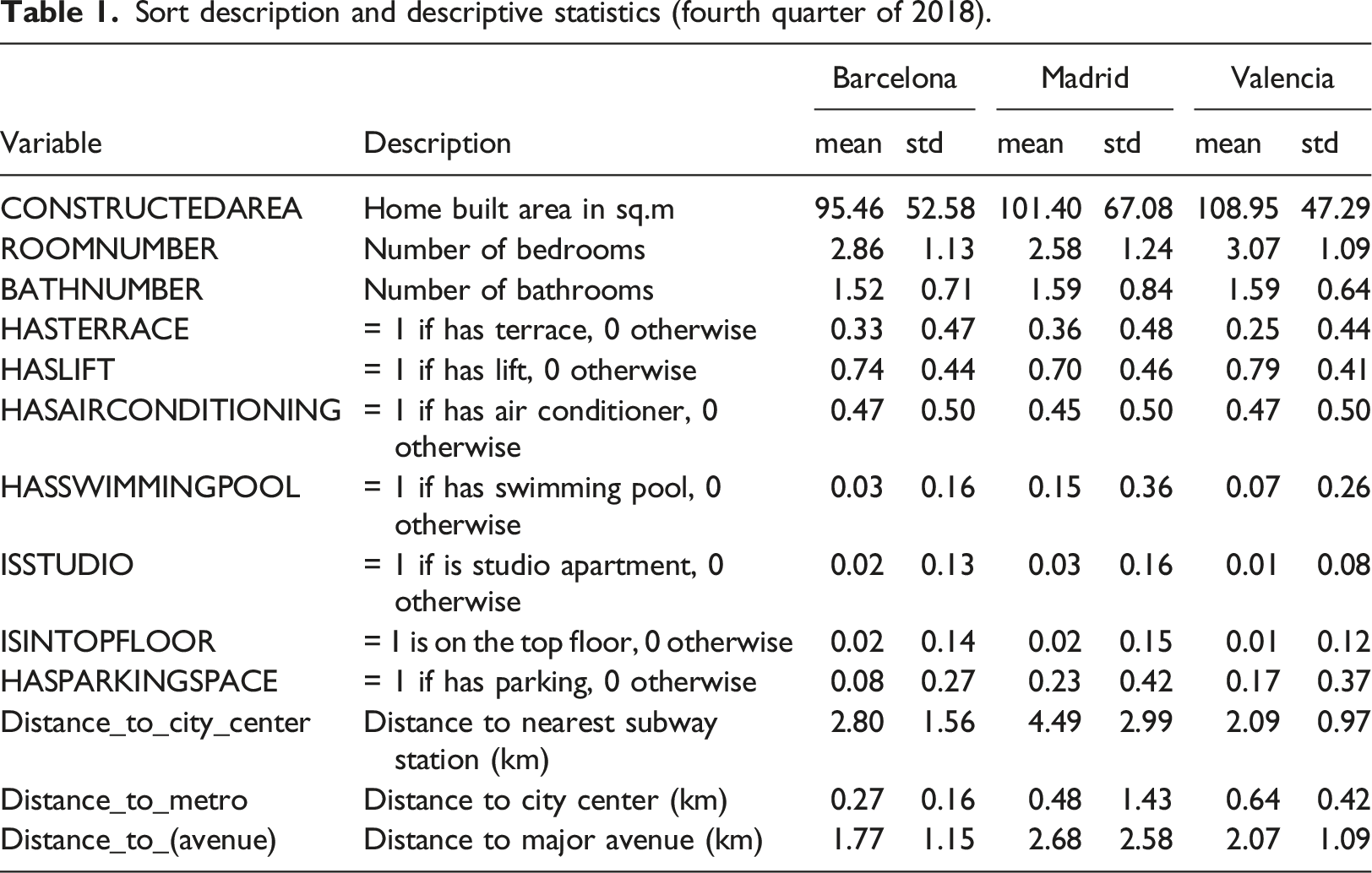
The data sets used in the analysis correspond to the last quarter of 2018 and include a total of n = 44,270 for Madrid, n = 23,334 for Barcelona, and n = 14,018 for Valencia. The distribution of prices displays a long tail in all three cities, and following conventional practice it is log-transformed. The coordinates are converted from latitude and longitude to northing and easting in meters, and then rescaled and centered using the corresponding city’s Central Business District as a false origin. These transformations have no impact on the analysis, and rescaling and centering of the coordinates is necessary for the correct implementation of the interactive basis functions in decision trees (see Paez et al., 2019: pp. 188–189).

For this research we select thirteen explanatory variables. Of these, ten attributes are data provided by Idealista.com and represent key structural attributes of the properties. These are whether the property is a studio (a small type of bachelor apartment), whether it is on the top floor of the building, and its built area, number of rooms, number of baths, and presence of a terrace. In addition, there are variables for elevator in the building, air conditioner, swimming pool, and parking spaces. We augment these attributes with locational variables derived from the coordinates of the property, including distance to nearest major transit station (metro), distance to the city center (central business district; CBD), and distance to major avenues. These locational attributes are frequently advertised by real estate agents and often capitalized in housing prices. Table 1 gives the definitions of these variables and the descriptive statistics of the data.

Table 1.

Sort description and descriptive statistics (fourth quarter of 2018).

Variable	Description	Barcelona		Madrid		Valencia
Variable	Description	mean	std	mean	std	mean	std
CONSTRUCTEDAREA	Home built area in sq.m	95.46	52.58	101.40	67.08	108.95	47.29
ROOMNUMBER	Number of bedrooms	2.86	1.13	2.58	1.24	3.07	1.09
BATHNUMBER	Number of bathrooms	1.52	0.71	1.59	0.84	1.59	0.64
HASTERRACE	= 1 if has terrace, 0 otherwise	0.33	0.47	0.36	0.48	0.25	0.44
HASLIFT	= 1 if has lift, 0 otherwise	0.74	0.44	0.70	0.46	0.79	0.41
HASAIRCONDITIONING	= 1 if has air conditioner, 0 otherwise	0.47	0.50	0.45	0.50	0.47	0.50
HASSWIMMINGPOOL	= 1 if has swimming pool, 0 otherwise	0.03	0.16	0.15	0.36	0.07	0.26
ISSTUDIO	= 1 if is studio apartment, 0 otherwise	0.02	0.13	0.03	0.16	0.01	0.08
ISINTOPFLOOR	= 1 is on the top floor, 0 otherwise	0.02	0.14	0.02	0.15	0.01	0.12
HASPARKINGSPACE	= 1 if has parking, 0 otherwise	0.08	0.27	0.23	0.42	0.17	0.37
Distance_to_city_center	Distance to nearest subway station (km)	2.80	1.56	4.49	2.99	2.09	0.97
Distance_to_metro	Distance to city center (km)	0.27	0.16	0.48	1.43	0.64	0.42
Distance_to_(avenue)	Distance to major avenue (km)	1.77	1.15	2.68	2.58	2.07	1.09

Empirical examples

Experimental design

Each city’s data set is split into a training sample and a testing sample using a 7:3 proportion. The training samples are used to estimate the models and the testing samples are used to assess the out-of-sample performance of the models.

We consider four models. First is a Base Model

y_{i} = \sum_{j = 1}^{k} β_{j} x_{i j} + ϵ_{i} (i = 1, \dots, n)

(1)

The second is a base model with market segments (Base Model + MS)

y_{i} = \sum_{m = 2}^{M} γ_{m} I (y_{i} \in R_{m}) + \sum_{j = 1}^{k} β_{j} x_{i j} + ϵ_{i} (i = 1, \dots, n)

(2)

The third is a spatial lag model (Spatial Model)

y_{i} = ρ \frac{1}{n_{i}} \sum_{j = 1}^{n_{i}} y_{j} + \sum_{j = 1}^{k} β_{j} x_{i j} + ϵ_{i} (i = 1, \dots, n)

(3)

And finally, the most general is a spatial lag model with market segments (Spatial Model + MS)

y_{i} = ρ \frac{1}{n_{i}} \sum_{j = 1}^{n_{i}} y_{j} + \sum_{m = 2}^{M} γ_{m} I (y_{i} \in R_{m}) + \sum_{j = 1}^{k} β_{j} x_{i j} + ϵ_{i} (i = 1, \dots, n)

(4)

Please note that all models nest in the Spatial Model + MS depending on what restrictions are placed on the parameters. In the Base Model

ρ = γ_{m} = 0 (\forall m)

(5)

In the Base Model + MS

ρ = 0

(6)

And in the Spatial Model

γ_{m} = 0 (\forall m)

(7)

Spatial weights matrices are constructed using a kth-nearest neighbor criterion, with k = 6 since this approximates the mean degree of connectivity in planar systems (Farber et al., 2009, Table 1). The spatial weights matrices are row-standardized before use in the models. With respect to the interactive basis functions for the decision trees, we consider the following functions (see supplementary material) with u and v as the planar coordinates of the observations, easting and northing, respectively

\begin{array}{c} u_{i} + v_{i} \\ u_{i}^{2} + v_{i}^{2} \\ u_{i} \cdot v_{i} \end{array}

(8)

We first look at the estimated models before discussing the in- and out-of-sample predictive performance of the models.

Modelling results

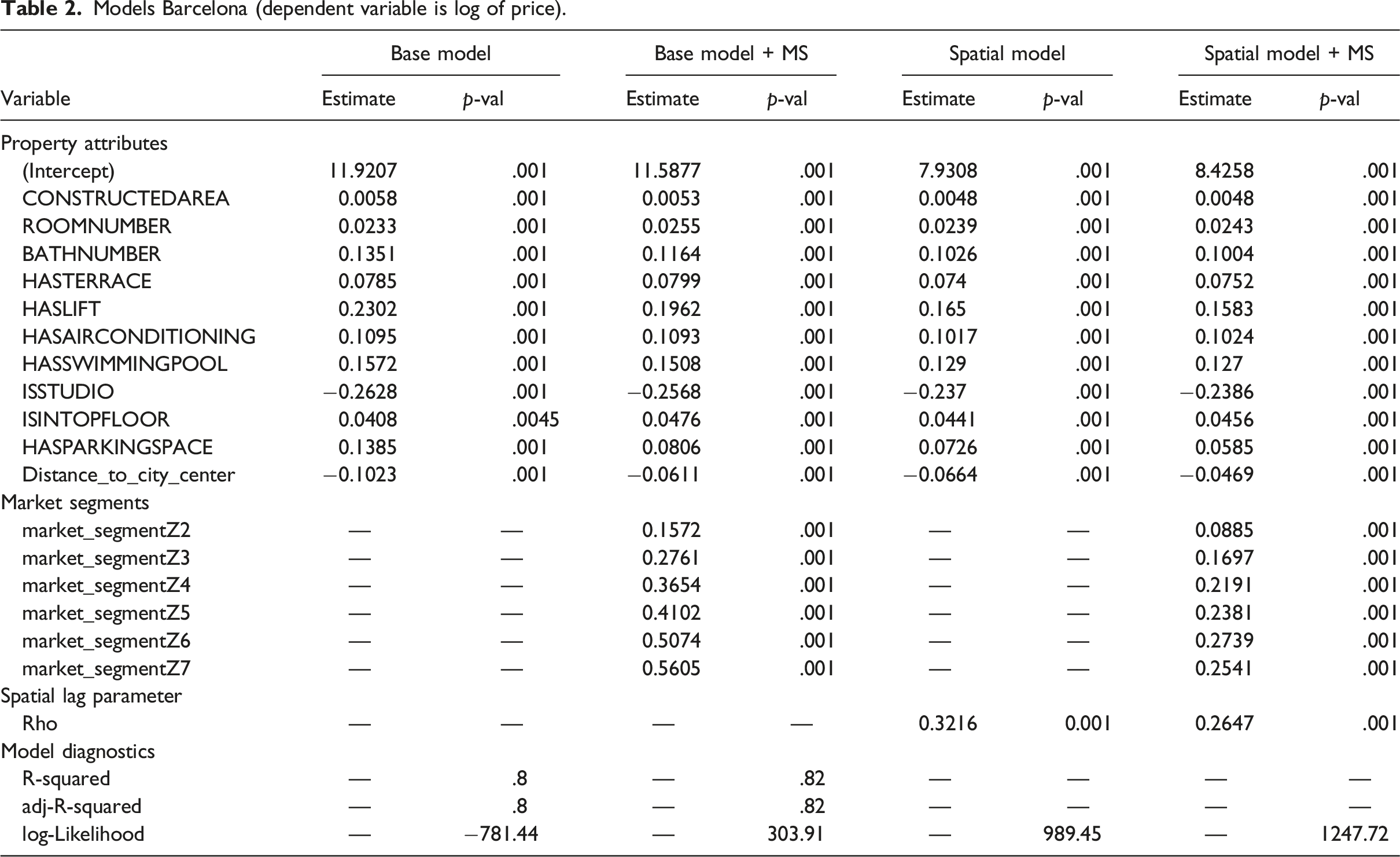
The first model in each of Tables 2 –4 is the Base Model. The fit of these models is reasonably high: the adjusted coefficients of determination are R² = 0.796, R² = 0.777, and R² = 0.795 for Barcelona, Madrid, and Valencia, respectively. These models are relatively naive in that they disregard both the possibility of spatial autocorrelation and spatial heterogeneity (in the form of spatial market sub-segments). They do provide a useful benchmark to compare the proposed modelling strategy.

Table 2.

Models Barcelona (dependent variable is log of price).

Variable	Base model		Base model + MS		Spatial model		Spatial model + MS
Variable	Estimate	p-val	Estimate	p-val	Estimate	p-val	Estimate	p-val
Property attributes
(Intercept)	11.9207	.001	11.5877	.001	7.9308	.001	8.4258	.001
CONSTRUCTEDAREA	0.0058	.001	0.0053	.001	0.0048	.001	0.0048	.001
ROOMNUMBER	0.0233	.001	0.0255	.001	0.0239	.001	0.0243	.001
BATHNUMBER	0.1351	.001	0.1164	.001	0.1026	.001	0.1004	.001
HASTERRACE	0.0785	.001	0.0799	.001	0.074	.001	0.0752	.001
HASLIFT	0.2302	.001	0.1962	.001	0.165	.001	0.1583	.001
HASAIRCONDITIONING	0.1095	.001	0.1093	.001	0.1017	.001	0.1024	.001
HASSWIMMINGPOOL	0.1572	.001	0.1508	.001	0.129	.001	0.127	.001
ISSTUDIO	−0.2628	.001	−0.2568	.001	−0.237	.001	−0.2386	.001
ISINTOPFLOOR	0.0408	.0045	0.0476	.001	0.0441	.001	0.0456	.001
HASPARKINGSPACE	0.1385	.001	0.0806	.001	0.0726	.001	0.0585	.001
Distance_to_city_center	−0.1023	.001	−0.0611	.001	−0.0664	.001	−0.0469	.001
Market segments
market_segmentZ2	—	—	0.1572	.001	—	—	0.0885	.001
market_segmentZ3	—	—	0.2761	.001	—	—	0.1697	.001
market_segmentZ4	—	—	0.3654	.001	—	—	0.2191	.001
market_segmentZ5	—	—	0.4102	.001	—	—	0.2381	.001
market_segmentZ6	—	—	0.5074	.001	—	—	0.2739	.001
market_segmentZ7	—	—	0.5605	.001	—	—	0.2541	.001
Spatial lag parameter
Rho	—	—	—	—	0.3216	0.001	0.2647	.001
Model diagnostics
R-squared	—	.8	—	.82	—	—	—	—
adj-R-squared	—	.8	—	.82	—	—	—	—
log-Likelihood	—	−781.44	—	303.91	—	989.45	—	1247.72

Table 3.

Models Madrid (dependent variable is log of price).

Variable	Base model		Base model + MS		Spatial model		Spatial model + MS
Variable	Estimate	p-val	Estimate	p-val	Estimate	p-val	Estimate	p-val
Property attributes
(Intercept)	11.8006	0.001	11.318	.001	5.9368	.001	8.1051	.001
CONSTRUCTEDAREA	0.0055	.001	0.0045	.001	0.0038	.001	0.0039	.001
ROOMNUMBER	−0.0068	.0087	0.0345	.001	0.0223	.001	0.0368	.001
BATHNUMBER	0.1653	.001	0.1163	.001	0.0999	.001	0.0958	.001
HASTERRACE	−0.0098	.0265	0.0459	.001	0.0202	.001	0.0436	.001
HASLIFT	0.3809	.001	0.2527	.001	0.2175	.001	0.2022	.001
HASAIRCONDITIONING	0.1036	.001	0.0878	.001	0.0871	.001	0.0841	.001
HASSWIMMINGPOOL	0.2119	.001	0.1961	.001	0.0895	.001	0.129	.001
ISSTUDIO	−0.1746	.001	−0.1827	.001	−0.1497	.001	−0.1671	.001
ISINTOPFLOOR	0.0256	.0565	0.0225	.0233	0.0361	.001	0.0296	.0012
HASPARKINGSPACE	0.0885	.001	0.1197	.001	0.0598	.001	0.0915	.001
Distance_to_metro	0.033	.001	−0.0414	.001	−0.0065	.001	−0.0394	.001
Distance_to_city_center	−0.0474	.001	−0.0484	.001	−0.0301	.001	−0.0394	.001
Distance_to_castellana	−0.0631	.001	0.0195	.001	−0.0215	.001	0.0175	.001
Market segments
market_segmentZ2	—	—	0.0663	.001	—	—	0.047	.001
market_segmentZ3	—	—	0.2286	.001	—	—	0.1643	.001
market_segmentZ4	—	—	0.4721	.001	—	—	0.3385	.001
market_segmentZ5	—	—	0.4969	.001	—	—	0.3501	.001
market_segmentZ6	—	—	0.5343	.001	—	—	0.366	.001
market_segmentZ7	—	—	0.7173	.001	—	—	0.4814	.001
market_segmentZ8	—	—	0.7399	.001	—	—	0.4986	.001
market_segmentZ9	—	—	0.9617	.001	—	—	0.6203	.001
Spatial lag parameter
ρ	—	—	—	—	0.4789	0.001	0.275	.001
Model diagnostics
R-squared	—	0.78	—	0.88	—	—	—	—
adj-R-squared	—	0.78	—	0.88	—	—	—	—
log-Likelihood	—	−12,024.16	—	−2623.16	—	−4050.73	—	−338.92

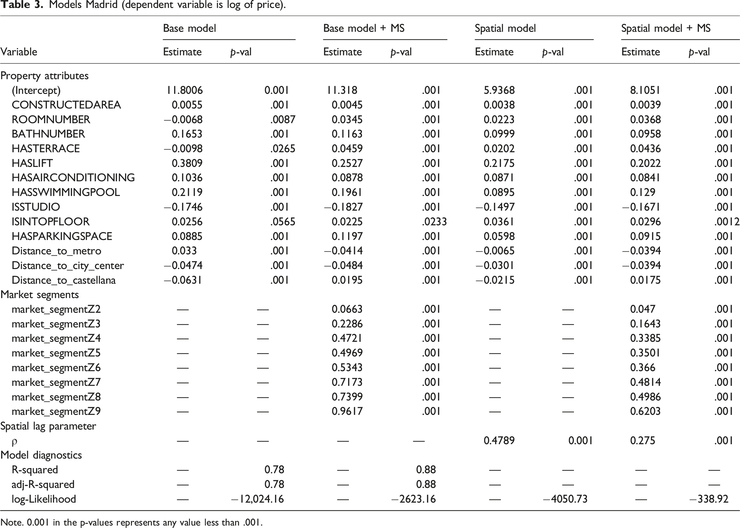
Note. 0.001 in the p-values represents any value less than .001.

Table 4.

Models Valencia (dependent variable is log of price).

Variable	Base model		Base model + MS		Spatial model		Spatial model + MS
Variable	Estimate	p-val	Estimate	p-val	Estimate	p-val	Estimate	p-val
Property attributes
(Intercept)	11.4979	.001	10.8973	.001	6.5688	.001	7.1013	.001
CONSTRUCTEDAREA	0.0066	.001	0.006	.001	0.0052	.001	0.0051	.001
ROOMNUMBER	−0.0528	.001	−0.0392	.001	−0.0393	.001	−0.0339	.001
BATHNUMBER	0.1619	.001	0.1461	.001	0.128	.001	0.1269	.001
HASTERRACE	0.0832	.001	0.0872	.001	0.0723	.001	0.0756	.001
HASLIFT	0.3022	.001	0.3118	.001	0.2231	.001	0.2457	.001
HASAIRCONDITIONING	0.1139	.001	0.1047	.001	0.096	.001	0.093	.001
HASSWIMMINGPOOL	0.3738	.001	0.3418	.001	0.1742	.001	0.1937	.001
ISSTUDIO	−0.0519	.1331	−0.0727	.0206	−0.042	.1493	−0.0589	.0342
ISINTOPFLOOR	0.074	.0023	0.092	.001	0.1104	.001	0.1157	.001
HASPARKINGSPACE	0.1301	.001	0.1482	.001	0.0961	.001	0.1135	.001
Distance_to_city_center	−0.1556	.001	−0.057	.001	−0.0695	.001	−0.0271	.001
Distance_to_metro	−0.1506	.001	−0.1061	.001	−0.0651	.001	−0.0585	.001
DISTANCE_TO_BLASCO	−0.1263	.001	−0.0806	.001	−0.0679	.001	−0.0514	.001
Market segments
market_segmentZ2	—	—	0.2071	.001	—	—	0.1018	.001
market_segmentZ3	—	—	0.3544	.001	—	—	0.2164	.001
market_segmentZ4	—	—	0.4348	.001	—	—	0.2514	.001
market_segmentZ5	—	—	0.3271	.001	—	—	0.164	.001
market_segmentZ6	—	—	0.6119	.001	—	—	0.3907	.001
market_segmentZ7	—	—	0.6346	.001	—	—	0.3635	.001
market_segmentZ8	—	—	0.7518	.001	—	—	0.3814	.001
Spatial lag parameter
ρ	—	—	—	—	0.4031	0.001	0.3314	.001
Model diagnostics
R-squared	—	0.79	—	0.83	—	—		—
adj-R-squared	—	0.79	—	0.83	—	—		—
log-Likelihood	—	−2282.65	—	−1343.2	—	−830.93		−449.46

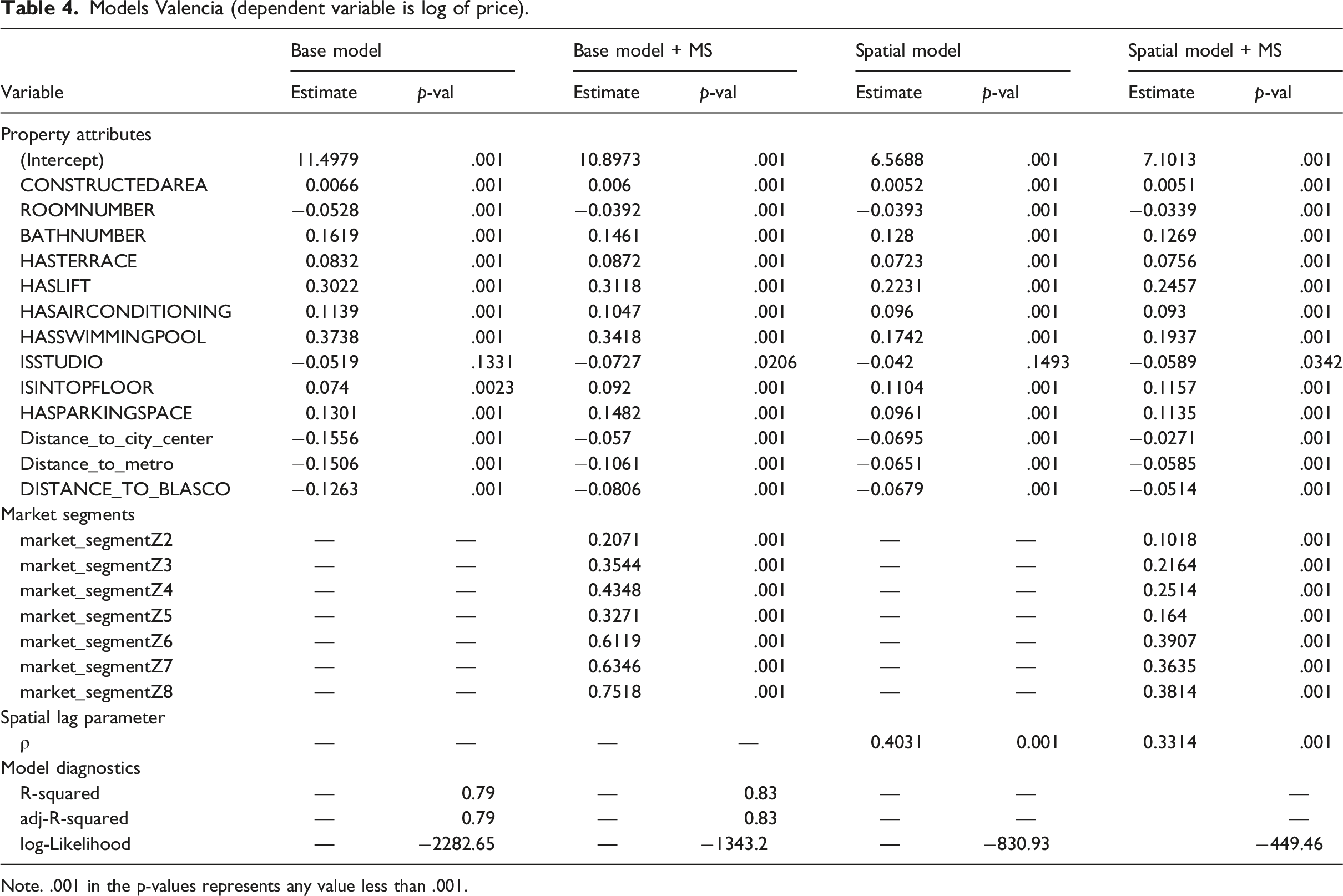
Note. .001 in the p-values represents any value less than .001.

Figure 1.

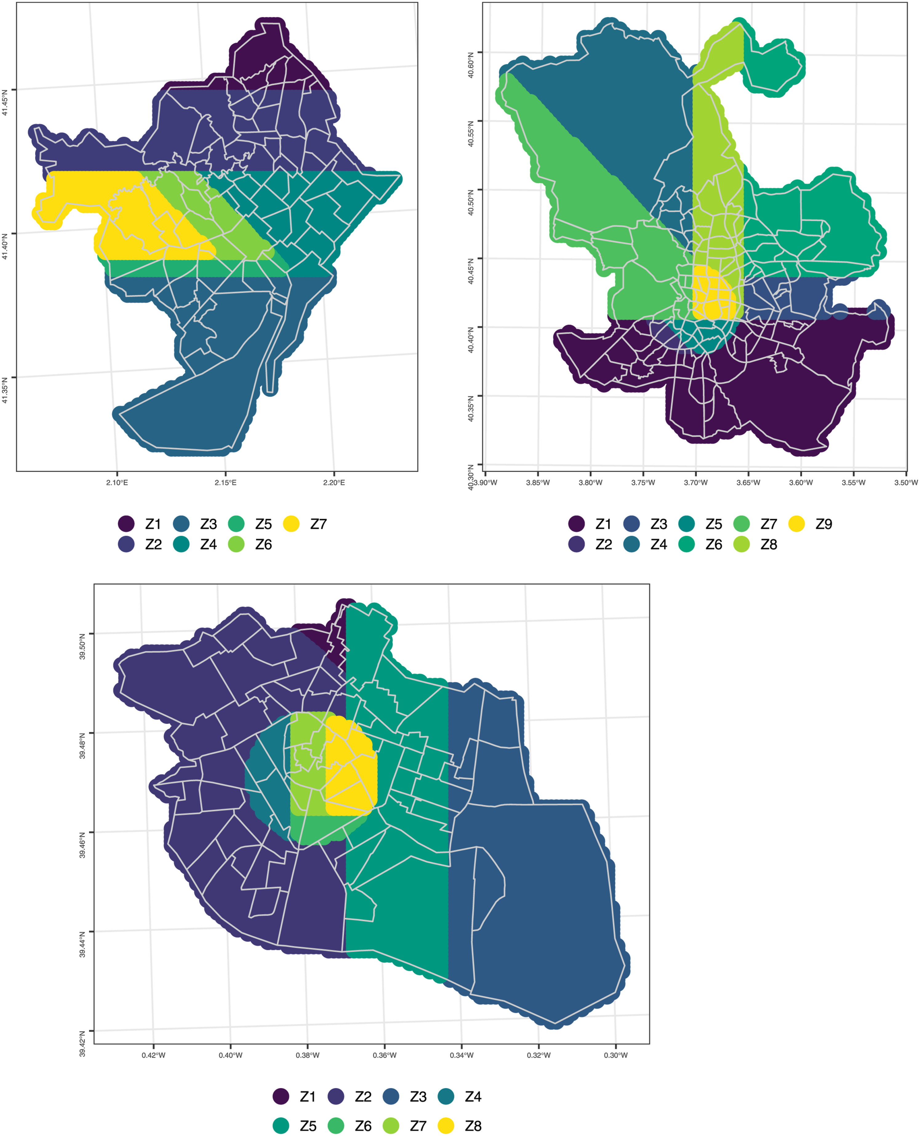
Spatial market segments according to Stage 1 classification tree. Barcelona (upper-left), Madrid (upper-right), and Valencia (bottom-center).

The first stage of the modelling strategy is to train a decision tree on the property values using only the coordinates of the observations. The spatial market sub-segments derived from the decision trees are shown in Figure 1. It can be seen there that the algorithm detects seven market sub-segments in Barcelona, nine market sub-segments in Madrid, and eight in Valencia. These submarkets are compact, mutually exclusive, and collectively exhaustive. The smallest market segment is found in Valencia and has 331 recorded transactions; the largest market segment, in contrast, has 7816 recorded transactions and is found in Madrid. The figures show how the use of interactive basis functions leads to flexible boundaries for the sub-markets. In the case of Barcelona, there are some distinctive diagonal shapes reminiscent of the street pattern in the city. In Madrid there is a clear distinction given by the M-30 orbital that surrounds the central almond of the city; in addition, there is Paseo de la Castellana, a major north-south avenue that crosses the city. This avenue divides two zones in the north that tend to include more expensive real estate, whereas the south tends to be lower income and less expensive. In Valencia, the sub-markets identify several zones in the historical center of the city, and then larger regional patterns depending on proximity to the waterfront to the west of the city.

The spatial market sub-segments are coded as dummy variables in the data sets before re-estimating the Base Model with market segments (Base Model + MS). The second model reported in Tables 2 –4 shows that the market segments tend to be highly significant, and also improve the fit of the model. In the case of Barcelona, the adjusted coefficient of determination changes to R² = 0.821, for a modest increase of 3.19%. The introduction of the market segments into the Base Model for Madrid results in an adjusted coefficient of determination of R² = 0.878, which represents a change of 13.09% relative to the adjusted coefficient of determination of the Base Model. In Valencia, the Base Model with market segments has an adjusted coefficient of determination of R² = 0.83, for an increase with respect to the Base Model of 4.49%.

It is well-known that spatial heterogeneity and association can co-exist (e.g., Bourassa et al., 2007; Paez et al., 2001). Sub-market identification can assist with spatial heterogeneity, but a process of spatial association could result from the common heuristic of comparative sales used by real estate agents. This process is appropriately represented by a spatial lag model. The third model reported in Tables 2 –4 is the Spatial Model, that is the Base Model with a spatial lag (i.e., Equation (3)). Spatial lag models, being non-linear, lack the coefficient of determination of linear regression. Instead, their goodness of fit is evaluated using likelihood measures. It can be seen that there is a substantial improvement in this regard in all three cities. The spatial lag parameter ρ represents the proportion of the mean of the neighboring prices that is reflected in the price of the property at i. In Barcelona, this parameter suggests that approximately 32.16% of the mean of the price of the k = 6 nearest neighbors is reflected in the price at i. This “comparative sales” effect is markedly stronger in Madrid, where it amounts to 47.89% of the mean price of the neighbors. In Valencia, this effect is 40.31%. The spatial lag parameter is significant in all three cases, and the results suggest that comparisons with other properties play a larger role in the determination of prices in Madrid.

The last model that we consider for these case studies is a spatial lag model with market segments. This is the most general of the four models, and we see that the combination of market segments and a spatial lag variable gives the best fit in terms of the log-likelihood, and also reduces the size of the spatial lag coefficient, shifting some of the spatial effect from spatial autocorrelation to spatial heterogeneity.

It is important to note that the coefficients of models with spatial lags cannot be interpreted as marginal effects due to the ripple effects of lagging variables. Instead, the direct, indirect, and total impacts need to be considered. The impacts of our best models (spatial models with market segments) are presented in Tables 5 –7.

Table 5.

Impacts spatial model + MS Barcelona (dependent variable is log of price).

Variable	Direct	p-val	Indirect	p-val	Total	p-val
Property attributes
CONSTRUCTEDAREA	0.005	.001	0.002	.001	0.007	.001
ROOMNUMBER	0.025	.001	0.009	.001	0.033	.001
BATHNUMBER	0.101	.001	0.035	.001	0.137	.001
HASTERRACE	0.076	.001	0.026	.001	0.102	.001
HASLIFT	0.160	.001	0.055	.001	0.215	.001
HASAIRCONDITIONING	0.103	.001	0.036	.001	0.139	.001
HASSWIMMINGPOOL	0.128	.001	0.044	.001	0.173	.001
ISSTUDIO	−0.241	.001	−0.084	.001	−0.324	.001
ISINTOPFLOOR	0.046	.001	0.016	.001	0.062	.001
HASPARKINGSPACE	0.059	.001	0.021	.001	0.080	.001
Distance_to_city_center	−0.047	.001	−0.016	.001	−0.064	.001
Market segments
market_segmentZ2	0.089	.001	0.031	.001	0.120	.001
market_segmentZ3	0.171	.001	0.059	.001	0.231	.001
market_segmentZ4	0.221	.001	0.077	.001	0.298	.001
market_segmentZ5	0.240	.001	0.083	.001	0.324	.001
market_segmentZ6	0.277	.001	0.096	.001	0.373	.001
market_segmentZ7	0.257	.001	0.089	.001	0.346	.001

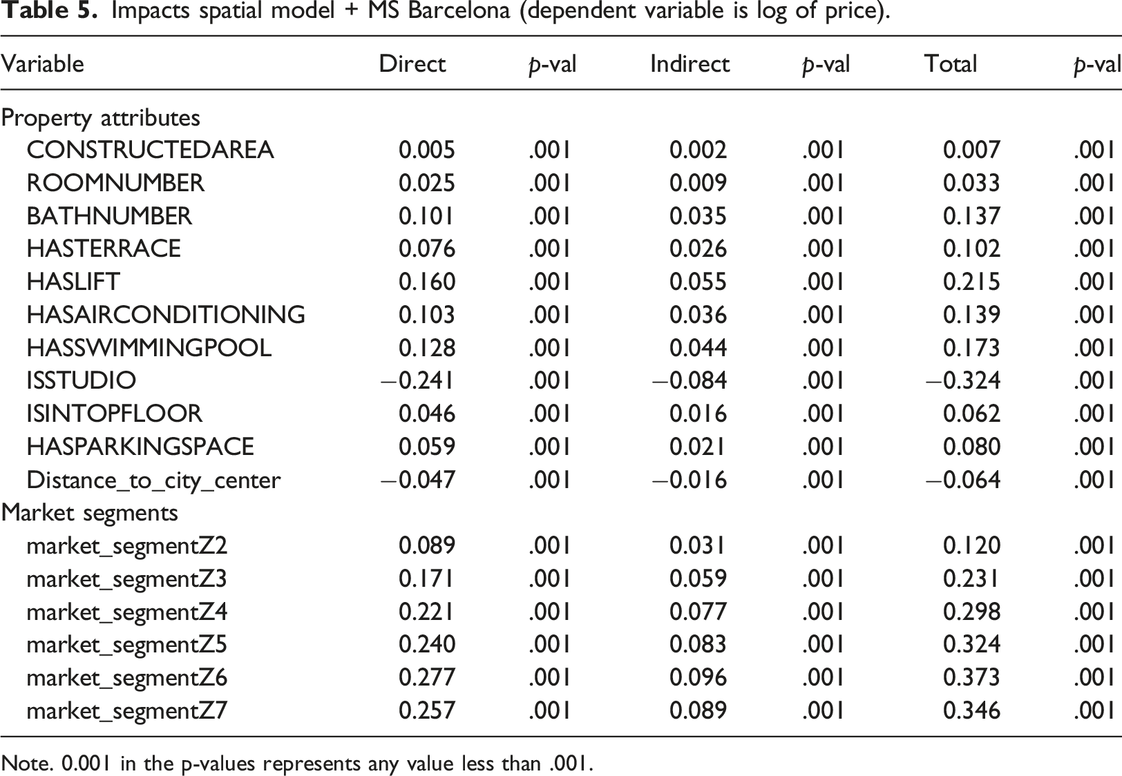
Note. 0.001 in the p-values represents any value less than .001.

Table 6.

Impacts Spatial Model + MS Madrid (dependent variable is log of price).

Variable	Direct	p-val	Indirect	p-val	Total	p-val
Property attributes
CONSTRUCTEDAREA	0.004	.001	0.001	.001	0.005	.001
ROOMNUMBER	0.037	.001	0.014	.001	0.051	.001
BATHNUMBER	0.096	.001	0.036	.001	0.132	.001
HASTERRACE	0.044	.001	0.016	.001	0.060	.001
HASLIFT	0.203	.001	0.076	.001	0.279	.001
HASAIRCONDITIONING	0.085	.001	0.031	.001	0.116	.001
HASSWIMMINGPOOL	0.130	.001	0.048	.001	0.178	.001
ISSTUDIO	−0.168	.001	−0.062	.001	−0.230	.001
ISINTOPFLOOR	0.030	.002	0.011	.002	0.041	.002
Hasparkingspace	0.092	.001	0.034	.001	0.126	.001
Distance_to_metro	−0.040	.001	−0.015	.001	−0.054	.001
Distance_to_city_center	−0.040	.001	−0.015	.001	−0.054	.001
Distance_to_castellana	0.018	.001	0.007	.001	0.024	.001
Market segments
market_segmentZ2	0.047	.001	0.018	.001	0.065	.001
market_segmentZ3	0.165	.001	0.061	.001	0.227	.001
market_segmentZ4	0.340	.001	0.127	.001	0.467	.001
market_segmentZ5	0.352	.001	0.131	.001	0.483	.001
market_segmentZ6	0.368	.001	0.137	.001	0.505	.001
market_segmentZ7	0.484	.001	0.180	.001	0.664	.001
market_segmentZ8	0.501	.001	0.186	.001	0.688	.001
market_segmentZ9	0.624	.001	0.232	.001	0.856	.001

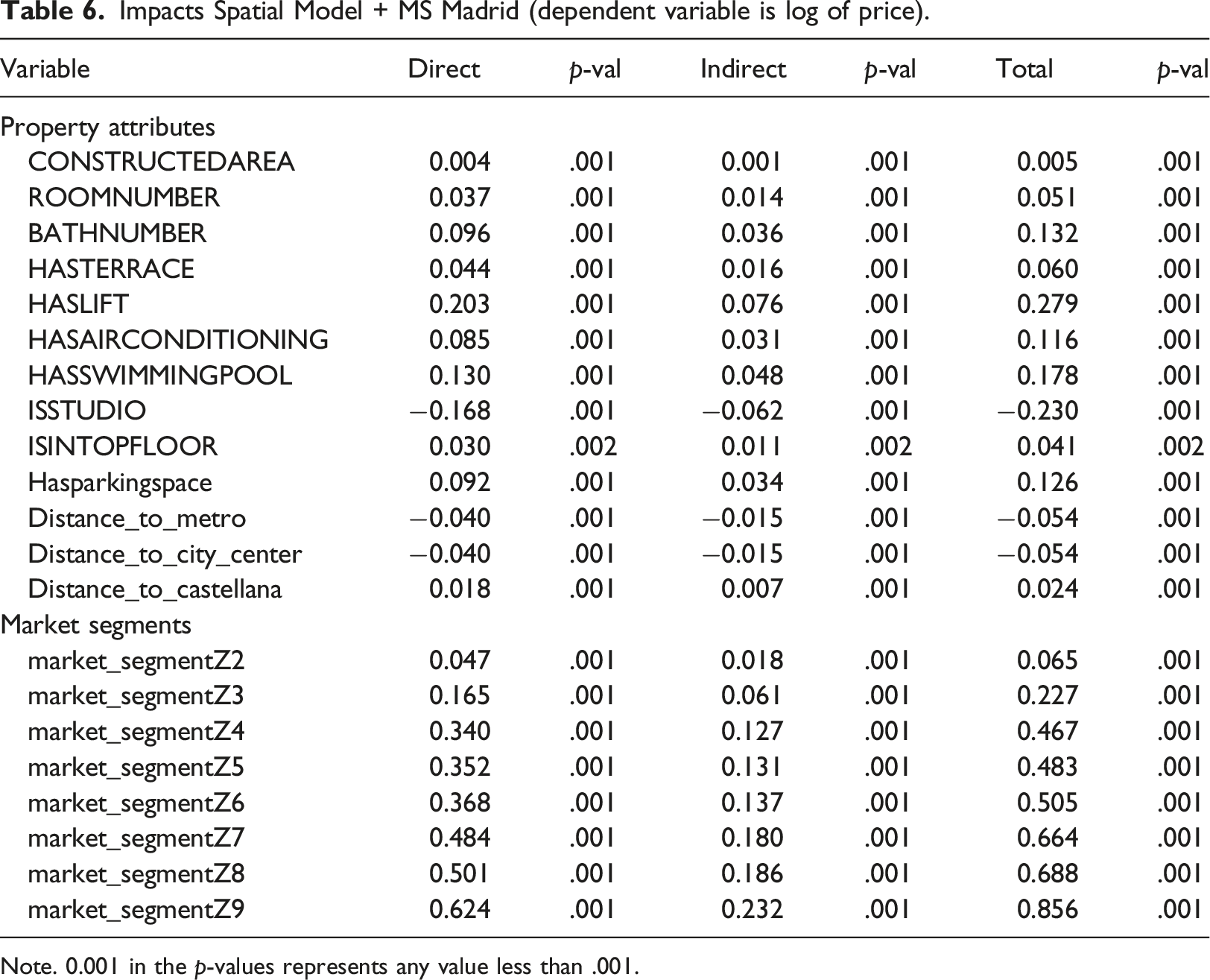
Note. 0.001 in the p-values represents any value less than .001.

Table 7.

Impacts spatial model + MS Valencia (dependent variable is log of price).

Variable	Direct	p-val	Indirect	p-val	Total	p-val
Property attributes
CONSTRUCTEDAREA	0.005	.001	0.002	.001	0.008	0.001
ROOMNUMBER	−0.035	.001	−0.016	.001	−0.051	0.001
BATHNUMBER	0.130	.001	0.060	0.001	0.190	0.001
HASTERRACE	0.078	.001	0.035	0.001	0.113	0.001
HASLIFT	0.252	.001	0.115	0.001	0.367	0.001
HASAIRCONDITIONING	0.095	.001	0.044	0.001	0.139	0.001
HASSWIMMINGPOOL	0.199	.001	0.091	0.001	0.290	0.001
ISSTUDIO	−0.060	.041	−0.028	0.041	−0.088	0.041
ISINTOPFLOOR	0.119	.001	0.054	0.001	0.173	0.001
HASPARKINGSPACE	0.116	.001	0.053	0.001	0.170	0.001
Distance_to_city_center	−0.028	.001	−0.013	0.001	−0.040	0.001
Distance_to_metro	−0.060	.001	−0.027	0.001	−0.087	0.001
Distance_to_blasco	−0.053	.001	−0.024	0.001	−0.077	0.001
Market segments
market_segmentZ2	0.104	0.001	0.048	0.001	0.152	0.001
market_segmentZ3	0.222	0.001	0.102	0.001	0.324	0.001
market_segmentZ4	0.258	0.001	0.118	0.001	0.376	0.001
market_segmentZ5	0.168	0.001	0.077	0.001	0.245	0.001
market_segmentZ6	0.401	0.001	0.183	0.001	0.584	0.001
market_segmentZ7	0.373	0.001	0.171	0.001	0.544	0.001
market_segmentZ8	0.391	0.001	0.179	0.001	0.570	0.001

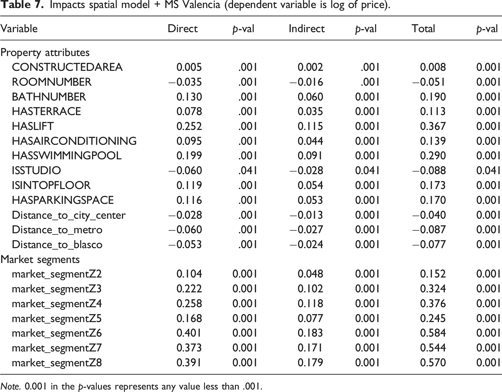
Note. 0.001 in the p-values represents any value less than .001.

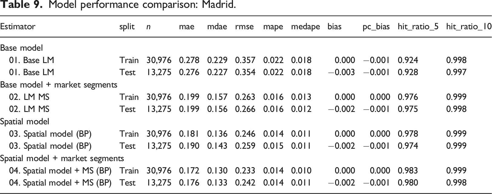
Predictive performance: comparison of models

Prediction is a relevant concern in hedonic price analysis. Inspection of the results in Tables 2 –4 suggest that the introduction of spatial market segments leads to markedly improved model fits. The measures of performance reported in these tables are based on the training sample exclusively. To conclude this investigation, in this section the predictive performance of the models is compared based on their performance using training (in-sample) as well as testing (out-of-sample) data sets. It is important to recall at this point that test data were not used in the calibration of the models discussed in the preceding sections.

The models without a spatially lagged dependent variable assume that the process is not spatially autocorrelated and therefore prediction requires only observations of the exogenous explanatory variables for the property to be assessed, since the price setting mechanism does not include information about the neighbors. In contrast, prediction with the models with a spatial lagged dependent variable require information regarding neighboring dependent and explanatory variables. This increases the data requirements and increases the computational complexity of prediction. Several approaches to spatial prediction with models that include spatially autocorrelated components are discussed in the literature (e.g., Goulard et al., 2017); these are discussed briefly next.

In case of model (4) two types of prediction based on the data can be considered: in- and out-of-sample predictions. In this paper we follow Goulard et al. (2017) proposal, as follows: we can reorder the observations in equation (4) to obtain the block matrix form below, where the subscript S denotes in-sample (training) data, and the subscript O out-of-sample (testing) data

[\begin{array}{c} Y_{S} \\ Y_{O} \end{array}] = ρ [\begin{array}{c} W_{S S} & W_{S O} \\ W_{O S} & W_{O O} \end{array}] [\begin{array}{c} Y_{S} \\ Y_{O} \end{array}] + [\begin{array}{c} X_{S} \\ X_{O} \end{array}] β + [\begin{array}{c} ϵ_{S} \\ ϵ_{O} \end{array}]

(9)

The best predictor (BP) approach is

{\hat{Y}}_{S}^{B P} = {\hat{Y}}_{S}^{T C} - d i a g {({\hat{Q}}_{S S})}^{- 1} ({\hat{Q}}_{S S} - d i a g ({\hat{Q}}_{S S})) (Y_{S} - {\hat{Y}}_{S}^{T C})

(10)

where

{\hat{Q}}_{S S} = 1 / {\hat{σ}}^{2} (I - \hat{ρ} W_{S S}^{'}) (I - \hat{ρ} W_{S S})

\hat{ρ}

is the in-sample spatial dependence estimate parameter and

{\hat{σ}}^{2}

is the estimate variance.

There are four alternatives for out-of-sample prediction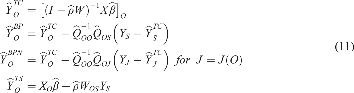

\begin{array}{c} {\hat{Y}}_{O}^{T C} = {[{(I - \hat{ρ} W)}^{- 1} X \hat{β}]}_{O} \\ {\hat{Y}}_{O}^{B P} = {\hat{Y}}_{O}^{T C} - {\hat{Q}}_{O O}^{- 1} {\hat{Q}}_{O S} (Y_{S} - {\hat{Y}}_{S}^{T C}) \\ {\hat{Y}}_{O}^{B P N} = {\hat{Y}}_{O}^{T C} - {\hat{Q}}_{O O}^{- 1} {\hat{Q}}_{O J} (Y_{J} - {\hat{Y}}_{J}^{T C}) f o r J = J (O) \\ {\hat{Y}}_{O}^{T S} = X_{O} \hat{β} + \hat{ρ} W_{O S} Y_{S} \end{array}

(11)

Of the four out-of-sample prediction methods we use the Best Predictor (BP) approach. Further detail on these alternatives can be found in Goulard et al. (2017). These prediction methods are implemented in the R package spatialreg (Bivand et al., 2013).

We use several metrics of performance for comparison. Tables 8 –10 report the mean absolute error (mae), median absolute prediction error (mdae), root mean squared error (rmse), mean absolute prediction error (mape), median absolute prediction error (medape), bias, percent bias (pc_bias), and hit rates. The latter are the proportion of predictions smaller than a given absolute deviation in percentage. For instance, the 5% hit rate (hit_rate_5) of the linear model for Barcelona is a 98%, therefore 98% of all observations have an absolute percent error smaller than a 5%.

Table 8.

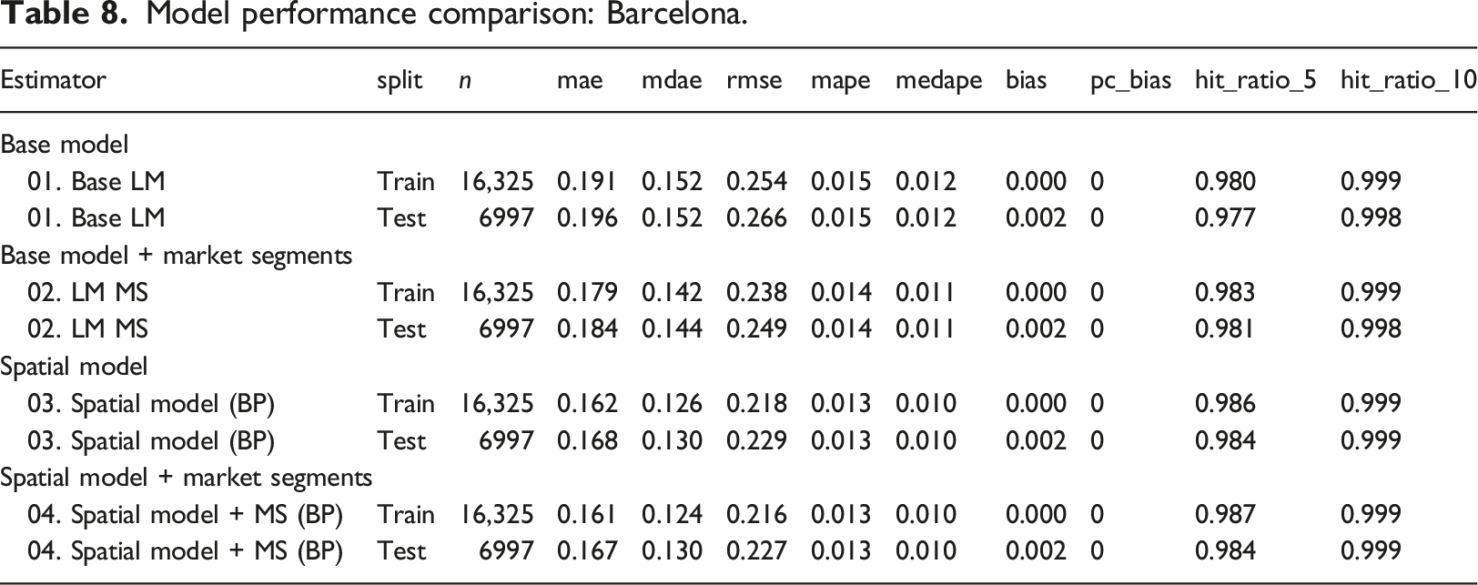
Model performance comparison: Barcelona.

Estimator	split	n	mae	mdae	rmse	mape	medape	bias	pc_bias	hit_ratio_5	hit_ratio_10
Base model
01. Base LM	Train	16,325	0.191	0.152	0.254	0.015	0.012	0.000	0	0.980	0.999
01. Base LM	Test	6997	0.196	0.152	0.266	0.015	0.012	0.002	0	0.977	0.998
Base model + market segments
02. LM MS	Train	16,325	0.179	0.142	0.238	0.014	0.011	0.000	0	0.983	0.999
02. LM MS	Test	6997	0.184	0.144	0.249	0.014	0.011	0.002	0	0.981	0.998
Spatial model
03. Spatial model (BP)	Train	16,325	0.162	0.126	0.218	0.013	0.010	0.000	0	0.986	0.999
03. Spatial model (BP)	Test	6997	0.168	0.130	0.229	0.013	0.010	0.002	0	0.984	0.999
Spatial model + market segments
04. Spatial model + MS (BP)	Train	16,325	0.161	0.124	0.216	0.013	0.010	0.000	0	0.987	0.999
04. Spatial model + MS (BP)	Test	6997	0.167	0.130	0.227	0.013	0.010	0.002	0	0.984	0.999

Table 9.

Model performance comparison: Madrid.

Estimator	split	n	mae	mdae	rmse	mape	medape	bias	pc_bias	hit_ratio_5	hit_ratio_10
Base model
01. Base LM	Train	30,976	0.278	0.229	0.357	0.022	0.018	0.000	−0.001	0.924	0.998
01. Base LM	Test	13,275	0.276	0.227	0.354	0.022	0.018	−0.003	−0.001	0.928	0.997
Base model + market segments
02. LM MS	Train	30,976	0.199	0.157	0.263	0.016	0.013	0.000	0.000	0.976	0.999
02. LM MS	Test	13,275	0.199	0.156	0.266	0.016	0.012	−0.002	−0.001	0.975	0.998
Spatial model
03. Spatial model (BP)	Train	30,976	0.181	0.136	0.246	0.014	0.011	0.000	0.000	0.978	0.999
03. Spatial model (BP)	Test	13,275	0.190	0.143	0.259	0.015	0.011	−0.002	−0.001	0.974	0.999
Spatial model + market segments
04. Spatial model + MS (BP)	Train	30,976	0.172	0.130	0.233	0.014	0.010	0.000	0.000	0.983	0.999
04. Spatial model + MS (BP)	Test	13,275	0.176	0.133	0.242	0.014	0.011	−0.002	−0.001	0.980	0.998

Table 10.

Model performance comparison: Valencia.

Estimator	split	n	mae	mdae	rmse	mape	medape	bias	pc_bias	hit_ratio_5	hit_ratio_10
Base model
01. Base LM	Train	9802	0.235	0.188	0.305	0.020	0.016	0.000	−0.001	0.950	0.998
01. Base LM	Test	4201	0.237	0.189	0.311	0.020	0.016	−0.001	−0.001	0.943	0.998
Base model + market segments
02. LM MS	Train	9802	0.212	0.170	0.278	0.018	0.014	0.000	−0.001	0.965	0.999
02. LM MS	Test	4201	0.216	0.176	0.285	0.018	0.015	0.000	−0.001	0.963	0.998
Spatial model
03. Spatial model (BP)	Train	9802	0.185	0.143	0.247	0.015	0.012	0.000	0.000	0.972	0.999
03. Spatial model (BP)	Test	4201	0.194	0.150	0.258	0.016	0.013	0.002	0.000	0.974	0.999
Spatial model + market segments
04. Spatial model + MS (BP)	Train	9802	0.183	0.143	0.243	0.015	0.012	0.000	0.000	0.976	0.999
04. Spatial model + MS (BP)	Test	4201	0.191	0.148	0.253	0.016	0.012	0.002	0.000	0.976	0.999

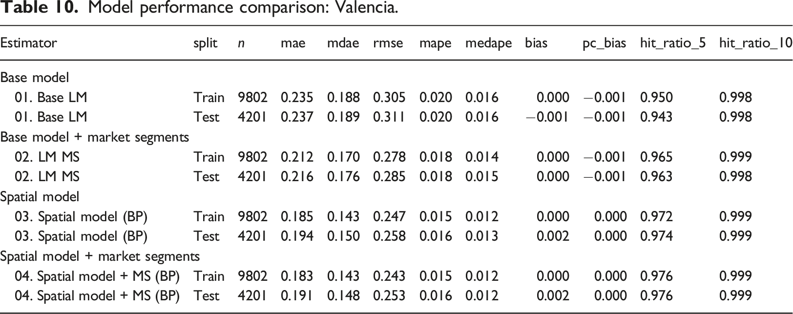
The results indicate that adding market segments and/or a spatially lagged variable improve the linear base model. The spatial model with market segments is comparable to or better than the spatial model without market segments. For example, the in- and out-of-sample predictions in Valencia perform very similarly in these two models. In Madrid and Valencia the results of the spatial model with market segment are superior for both the in-sample and the out-of-sample predictions.

Conclusions

Market segmentation is a topic of interest in the literature on real estate appraisal and valuation. In addition to being conceptually sound, numerous studies throughout the years have demonstrated that the practice of identifying market segments for hedonic price analysis can lead to higher quality models and enhanced performance.

The contribution of this paper has been to demonstrate a modelling strategy to obtain flexible tree-based market segments for use in spatial hedonic price modeling. Implementation of regression trees for market segmentation was proposed in a recent paper by Füss and Koller (2016). Our modelling strategy differs to the one proposed by these authors in two respects: 1) the use of decision trees with flexible (i.e., non-orthogonal and possibly non-linear market boundaries) and 2) the timing of the estimations of the market segments, which in the case of Füss and Koller (2016) is based on the residuals of an initial regression model, whereas in our case it is done in the first step of the modelling strategy.

The results using three large data sets from cities in Spain indicate that modelling the market segments can improve the fit of the models, as well as their predictive performance. The best model consistently included a spatially lagged dependent variable and market segments. The market segments in addition to improving the fit and the predictive performance also reduced the magnitude of the spatial lag parameter, thus allocating some of the spatial effect to regional heterogeneity that would otherwise be assumed to be micro-scale information spillovers. Overall, the results serve to demonstrate the potential of the proposed modelling strategy to produce better models and more accurate predictions.

One direction for future research is to investigate the temporal stability of spatial market segments. It is well known that there are seasonal effects in housing markets, but an open research question is whether spatial market segments experience seasonal variations, both in terms of their geographical extent as well as the magnitude of their effects. Another possibility is that there are longer term trends (e.g., gentrification) that could affect the spatial configuration of the market segments. Both seasonality and/or longer term trends would require multi-year data sets, compared to the single-year data set that we used for this research. For the time being, it is important to note that the results presented in this paper support the argument that the two-step method described in this paper performs well for now-casting or relatively short term forecasts. Given the dearth of information about seasonality and temporal stability of spatial market segments, any attempt to use them for longer term forecasts should be done with caution.

Finally, the study was designed as an example of reproducible research: all code and data used in this research is publicly available which should allow other researchers reproduce our results or expand them in other directions.

Supplemental Material

Supplemental Material - Using machine learning to identify spatial market segments. A reproducible study of major Spanish marketssj-pdf-1-epb-10.1177/2399808323116695

Using machine learning to identify spatial market segments. A reproducible study of major Spanish markets by David Rey-Blanco, Pelayo Arbues, Fernando Lopez and Antonio Paez in Environment and Planning B: Urban Analytics and City Science

Footnotes

Declaration of conflicting interests

The author(s) declared no potential conflicts of interest with respect to the research, authorship, and/or publication of this article.

Funding

The author(s) disclosed receipt of the following financial support for the research, authorship, and/or publication of this article: Fernando A. López acknowledge the financial support from project (PID2019-107800GB-I00).

ORCID iDs

David Rey-Blanco

Pelayo Arbués

Fernando A. López

Antonio Páez

Supplemental Material

Supplemental material for this article is available online.

Notes

David Rey currently works as Chief Data Officer at idealista, he is currently performing applied research in residential house price indices, as part of his Ph.D in economics work, at the UNED University in Spain. During the past twenty years, he has been working in several leading positions in technology and data science teams, along with launching several startups in the fields of advanced analytics and digital contents.

Pelayo Arbués is the Head of Data Science at idealista. He has a Ph.D. in Economics at the University of Oviedo. His research focuses on Transport Economics, Regional Science and Spatial Econometrics. He recieved the 2013 Juan Ramón Cuadrado Young Researchers Award.

Fernando A. López is a full professor at the Technical University of Cartagena (Spain). He focuses on spatial econometrics research, in which has published both methodological and applied paper. In the field of spatial econometric several topics has been analyzed: parametric instability of spatial regression models, clusters identification, spatial symbolic analysis and he has developed several tests of spatial dependence. Moreover, two R packages are available in CRAN to estimate spatial seemingly unrelated regression model (spsur) and for testing for spatial dependence in qualitative data (spqdep). Several of these works analyze spatial dependency structures in hedonic models.

Antonio Páez is a civil engineer by training and geographer by adoption. He is author or coauthor of more than 140 peer-reviewed papers in fields that include transportation, health geography, social networks, and regional science. He is co-author of Discrete Choice Analysis with R, published by Springer in its UseR! series.

References

Alonso

(1964) Location and Land Use. Cambridge: Harvard University Press.

Arribas-Bel

Green

Rowe

, et al. (2021) Open data products-a framework for creating valuable analysis ready data. Journal of Geographical Systems 23(4): 497–514.

Bivand

Pebesma

Gomez-Rubio

, et al. (2013) Applied Spatial Data Analysis with R. Berlin: Springer.

Bourassa

Cantoni

Hoesli

(2007) Spatial dependence, housing submarkets, and house price prediction. The Journal of Real Estate Finance and Economics 35(2): 143–160.

Cellmer

Kobylinska

Belej

(2019) Application of hierarchical spatial autoregressive models to develop land value maps in urbanized areas. Isprs International Journal of Geo-Information 8(4): 195.

Chasco

Le Gallo

López

(2018) A scan test for spatial groupwise heteroscedasticity in cross-sectional models with an application on houses prices in madrid. Regional Science and Urban Economics 68: 226–238.

Liu

(2019) Techniques for interpretable machine learning. Communications of the ACM 63(1): 68–77. DOI: 10.1145/3359786.

Farber

Paez

Volz

(2009) Topology and dependency tests in spatial and network autoregressive models. Geographical Analysis 41(2): 158–180.

Füss

Koller

(2016) The role of spatial and temporal structure for residential rent predictions. International Journal of Forecasting 32(4): 1352–1368.

10.

Galster

(1996) William grigsby and the analysis of housing sub-markets and filtering. Urban Studies 33(10): 1797–1805.

11.

Goulard

Laurent

Thomas-Agnan

(2017) About predictions in spatial autoregressive models: optimal and almost optimal strategies. Spatial Economic Analysis 12(2–3): 304–325.

12.

Helbich

Brunauer

Hagenauer

, et al. (2013) Data-driven regionalization of housing markets. Annals of the Association of American Geographers 103(4): 871–889.

13.

Helbich

Griffith

(2016) Spatially varying coefficient models in real estate: Eigenvector spatial filtering and alternative approaches. Computers Environment and Urban Systems 57: 1–11.

14.

Han

, et al. (2019) Monitoring housing rental prices based on social media: an integrated approach of machine-learning algorithms and hedonic modeling to inform equitable housing policies. Land Use Policy 82: 657–673.

15.

Humphreys

Nowak

Zhou

(2019) Superstition and real estate prices: transaction-level evidence from the us housing market. Applied Economics 51(26): 2818–2841.

16.

Hwang

Thill

(2009) Delineating urban housing submarkets with fuzzy clustering. Environment and Planning B: Planning and Design 36(5): 865–882.

17.

Islam

Asami

(2011) Addressing Structural Instability in Housing Market Segmentation of the Used Houses of Tokyo, Japan, Procedia Social and Behavioral Sciences. Amsterdam: Elsevier Science Bv.

18.

James

Witten

Hastie

, et al. (2013) An Introduction to Statistical Learning. Berlin: Springer,

19.

Knaus

Lechner

Strittmatter

(2021) Machine learning estimation of heterogeneous causal effects: empirical monte carlo evidence. The Econometrics Journal 24(1): 134–161. DOI: 10.1093/ectj/utaa014 DOI: 10.1093/ectj/utaa014.

20.

López

Minguez

Mur

(2020) Ml versus iv estimates of spatial sur models: evidence from the case of airbnb in madrid urban area. The Annals of Regional Science 64(2): 313–347.

21.

López

Chasco

Gallo

(2015) Exploring scan methods to test spatial structure with an application to housing prices in madrid. Papers in Regional Science 94(2): 317–346.

22.

Montero

Fernandez-Aviles

Minguez

(2018) Estimating environment impacts on housing prices. Environmetrics 29(5–6): e2453. DOI: 10.1002/env.2453.

23.

Montero-Lorenzo

Larraz-Iribas

Paez

(2009) Estimating commercial property prices: an application of cokriging with housing prices as ancillary information. Journal of Geographical Systems 11(4): 407–425.

24.

Morillo

García Cepeda

Martinez-Cuevas

(2016) The application of spatial analysis to cadastral zoning of urban areas: an example in the city of madrid. Survey Review 49(353): 1–10. DOI: 10.1080/00396265.2015.1113029.

25.

Murdoch

Singh

Kumbier

, et al. (2019) Definitions, methods, and applications in interpretable machine learning. Proceedings of the National Academy of Sciences of the United States of America 116(44): 22071–22080. DOI: 10.1073/pnas.1900654116 DOI: 10.1073/pnas.1900654116.

26.

Nowak

Sayago-Gomez

(2018) Homeowner preferences after september 11th, a microdata approach. Regional Science and Urban Economics 70: 330–351. DOI: 10.1016/j.regsciurbeco.2017.10.001.

27.

Pace

Barry

Clapp

, et al. (1998) Spatiotemporal autoregressive models of neighborhood effects. The Journal of Real Estate Finance and Economics 17(1): 15–33.

28.

Pace

Gilley

(1997) Using the spatial configuration of the data to improve estimation. The Journal of Real Estate Finance and Economics 14(3): 333–340.

29.

Paez

(2009) Recent research in spatial real estate hedonic analysis. Journal of Geographical Systems 11(4): 311–316.

30.

Paez

(2021) Open spatial sciences: an introduction. Journal of Geographical Systems 23(4): 467–476.

31.

Paez

López

Ruiz

, et al. (2019) Inducing non-orthogonal and non-linear decision boundaries in decision trees via interactive basis functions. Expert Systems with Applications 122: 183–206.

32.

Paez

Uchida

Miyamoto

(2001) Spatial association and heterogeneity issues in land price models. Urban Studies 38(9): 1493–1508.

33.

Paterson

Boyle

(2002) Out of sight, out of mind? using gis to incorporate visibility in hedonic property value models. Land Economics 78(3): 417–425.

34.

Páez

Long

Farber

(2008) Moving window approaches for hedonic price estimation: an empirical comparison of modelling techniques. Urban Studies 45(8): 1565–1581.

35.

Rapkin

Winnick

Blank

(1953) Housing Market Analysis. Washington: US Housing and Home Finance Agency.

36.

Ripley

(2021) Tree: Classification and Regression Trees. https://CRAN.R-project.org/package=tree. R package version 1.0-41.

37.

Rosen

(1974) Hedonic prices and implicit markets: product differentiation in pure competition. Journal of Political Economy 82(1): 34–55.

38.

Royuela

Duque

(2013) Housi: heuristic for delimitation of housing submarkets and price homogeneous areas. Computers Environment and Urban Systems 37: 59–69.

39.

Rudin

(2019) Stop explaining black box machine learning models for high stakes decisions and use interpretable models instead. Nature Machine Intelligence 1(5): 206–215. DOI:10.1038/s42256-019-0048-x.

40.

Thibodeau

(2003) Marking single-family property values to market. Real Estate Economics 31(1): 1–22.

41.

Unwin

(1978) An Introduction to Trend Surface Analysis, Concepts and Techniques in Modern Geography. Norwich: University of East Anglia.

42.

Usman

Lizam

Adekunle

(2020) Property price modelling, market segmentation and submarket classifications: a review. Real Estate Management and Valuation 28(3): 24–35.

43.

von Graevenitz

(2018) The amenity cost of road noise. Journal of Environmental Economics and Management 90: 1–22.

44.

Wager

Athey

(2018) Estimation and inference of heterogeneous treatment effects using random forests. Journal of the American Statistical Association 113(523): 1228–1242. DOI: 10.1080/01621459.2017.1319839.

45.

Watkins

(2001) The definition and identification of housing submarkets. Environment and Planning A: Economy and Space 33(12): 2235–2253.

46.

Wheeler

Paez

Spinney

, et al. (2014) A bayesian approach to hedonic price analysis. Papers in Regional Science 93(3): 663–683.

47.

Ren

, et al. (2018) Modified data-driven framework for housing market segmentation. Journal of Urban Planning and Development 144(4): 15.

48.

Yoo

Wagner

(2012) Variable selection for hedonic model using machine learning approaches: a case study in onondaga county, ny. Landscape and Urban Planning 107(3): 293–306.

Supplementary Material

Please find the following supplemental material available below.

For Open Access articles published under a Creative Commons License, all supplemental material carries the same license as the article it is associated with.

For non-Open Access articles published, all supplemental material carries a non-exclusive license, and permission requests for re-use of supplemental material or any part of supplemental material shall be sent directly to the copyright owner as specified in the copyright notice associated with the article.

0.00 MB

0.35 MB