History,neighborhood,and proximity as factors of land-use change: A dynamic spatial regression model

Abstract

Spatio-temporal land-use change (LUC) modeling provides vital information about land development dynamics. However, accounting for such dynamics faces methodological challenges. This research introduces a Dynamic Spatial Panel Data (DSPD) modeling framework for LUC, incorporating spatial and temporal dependencies. A continuous response variable is introduced to take advantage of traditional spatial regression models. The DSPD model is applied to balanced spatial panel data at the block-group level covering Florida between 2010 and 2019 and incorporating both new and previously used proxy variables. The urban growth impacts of site-specific, proximity, neighborhood, socio-economic, and transportation factors are investigated. This study contributes to the literature by providing extensive insights into spatial autocorrelation, spillover, heterogeneity, and temporal lag effects in urban growth. Also, the study reveals the importance of mobility and mortgage financing in land development. The proposed modeling framework achieves high accuracy. The dynamic structure of this model provides an opportunity to predict future urban growth without the need for a land development scenario. Such predictions provide insights about future land development to practitioners and policymakers.

Introduction

The main goal of land-use change (LUC) modeling is to mimic the complex land dynamics that lead to changes in urban and rural areas. Data-driven empirical approaches require extensive information to develop mathematical representations of urban and rural systems. Based on land economics theory, the current land-use status on a given parcel changes if the expected benefits from changing conditions minus the one-time conversion costs are larger than the benefits under current conditions. However, because the expected benefits cannot be directly estimated with the available information, proxy information is used to model these benefits. In earlier studies, LUC models have mainly included site-specific, proximity, neighborhood, socio-economic, and transportation factors, but there is no consensus regarding the selection of proxy information (Irwin and Geoghegan, 2001; Verburg et al., 2004). Bella and Irwin (2002) and Carrión-Flores and Irwin (2004) highlight the importance of spatially explicit LUC modeling using micro-level data. Carrión-Flores and Irwin (2004) control for the spatial autocorrelations in the error term. Nahuelhual et al. (2012) apply an autologistic regression approach to examine temporal dynamics in land development. Recent studies have also incorporated spatial and temporal dependencies because neighborhood and historical effects play critical roles in land dynamics (Deng and Srinivasan, 2016). Tepe and Guldmann (2017, 2020) introduce an autologistic regression methods explicitly accounting for spatial and temporal dependencies. Including these lags resolves the omitted variable bias problem in OLS regression-based LUC models.

The main goal of this study is to propose and estimate a Dynamic Spatial Panel Data (DSPD) model with both new and previously used proxy variables. This model explicitly quantifies spatial and temporal lagged relationships and incorporates site-specific, proximity, neighborhood, socio-economic, and transportation variables. Iacono et al. (2008) indicate that detailed characteristics of locations and residents should be included in LUC models because transportation impacts LUC through changes in accessibility and congestion. Also, traffic congestion creates negative externalities such as air and noise pollution in adjacent areas and endangers environmental systems. The model better represents human decision-making, using socio-economic indicators, such as population density, ethnicity, student and employment ratios, housing finance, and workers’ travel behaviors. Florida is selected as the case study area to evaluate the impacts of this proxy information. A balanced spatial panel data is derived from three primary data sources, and the details are presented in Section 4.

This study contributes to the existing literature in four ways by: (1) providing detailed insights about spatial and temporal lag effects in urban growth through the dependent variable, covariates, and residuals; (2) introducing a continuous response variable at the block-group (BG) level, in contrast to earlier discrete parcel information, thus enabling the implementation of traditional spatial regression modeling; (3) investigating the impacts of transportation infrastructure and mobility in land development by incorporating the distances to main roads and traffic volumes; (4) incorporating direct information about the demand for new real estate development, including mortgage financing and employment rates.

Literature review

The literature review on LUC modeling suggests that: (1) LUC results from the complex interactions between human activities and the built environment (Verburg et al., 2004); (2) Land-use models mimic complex land development dynamics (Noszczyk, 2019); (3) Incorporating spatial dependencies in LUC models is necessary to account for feedback mechanisms among neighbors (Munroe and Müller, 2007); (4) Historical trends are also essential in LUC models because certain historical conditions impact current and future land developments (Kim et al., 2022; Tepe and Guldmann, 2017, 2020; Tepe and Safikhani, 2023). The focus of this review is on recent statistical-based LUC models. Table 1 summarizes some details of recent studies, including data size, spatial and temporal components, geographical level, study area, and model accuracy.

Table 1.

Summary of LUC statistical models incorporating spatial and/or temporal components.

Study	Data size	Spatial	Temporal	Geographic levels	Study area	Model accuracy
Arsanjani et al. (2013)	N.A.	Yes	Not explicit	30 m × 30 m grid	Tehran, Iran	89.00%
Bhat et al. (2015)	2,383	Yes	Yes	0.25 mi × 0.25 mi grid	Austin, Texas	N.A.
Carrión-Flores and Irwin (2004)	4,000–6,000	Yes	Yes	Parcel	Medina, Ohio	85.2%, 85.4%, and 86.4%
Deng and Srinivasan (2016)	2,651	Yes	No	100 m × 100 m grid	Beijing, China	N.A.
Ferdous and Bhat (2013)	783	Yes	Yes	Parcel	Austin, Texas	N.A.
Gaur et al. (2020)	N.A.	Yes	Yes	30 m × 30 m grid	Subarnarekha basin, India	0.58–0.91% (AUC)
Hu and Lo (2007)	20,389	Yes	No	225 m × 225 m grid	Atlanta Metro, Georgia	85% (ROC)
Huang et al. (2009)	600–800	Yes	Not explicit	50 m × 50 m grid	New Castle, Delaware	68.52%, 71.13%, 75.62%
Irwin et al. (2003)	1,962	No	Yes	Parcel	Calvert County, Maryland	N.A.
Lavalle et al. (2011)	N.A.	Yes	No	100 m ×100 m grid	NUTS 2 regions, Europe	88.5%–96.5%
Liao and Wei (2014)	17,552	Yes	No	30 m × 30 m grid	Dongguan, China	81.9% (ROC)
Nahuelhual et al. (2012)	2,000	Yes	Not explicit	50 m × 50 m grid	South-Central Chile	69.20%
Tepe and Guldmann (2017)	72,069	Yes	Yes	Parcel	Delaware, Ohio	97.19%
Tepe and Guldmann (2020)	72,069	Yes	Yes	Parcel	Delaware, Ohio	91.40%

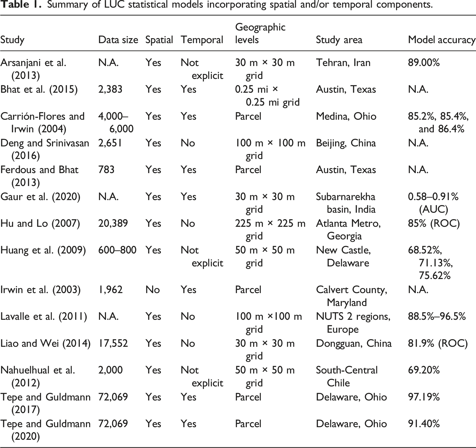
Spatial heterogeneity and clustering patterns are important driving factors in LUC (Arsanjani et al., 2013; Legendre and Legendre, 1998). Spatial dependencies must be controlled to improve model robustness and achieve efficient results. In some studies, spatial sampling is implemented to reduce spatial dependencies (Gaur et al., 2020; Hu and Lo, 2007; Jokar Arsanjani et al., 2013; Munroe and Müller, 2007). Bhat et al. (2015), Deng and Srinivasan (2016), and Hu and Lo (2007) use spatial lag components to control for spatial dependency. Similarly, temporal lagged components are used by Bhat et al. (2015), Huang et al. (2009), and Tepe and Guldmann (2017, 2020). Alternatively, Carrión-Flores & Irwin (2004) specify a simultaneous autoregressive process in the error terms of their residential land conversion model. Liao and Wei (2014) employ a logistic regression approach with spatially expanded coefficients to investigate the spatial complexities of urban growth in Dongguan, China. The EUCS100 model (Lavalle et al., 2011) implements a standard multinomial logit for simulating LUC dynamics in the European region but does not account for the endogeneity of the interactions among the land-use variables across spatial units.

Temporal dependencies are also crucial in LUC dynamics, but few studies have incorporated temporal dynamics in their models. Huang et al. (2009) apply a logistic regression for urban expansion and implement exponentially decreasing weights for older observations to integrate bi-temporal land-use models over three periods between the 1980s and 2000s. Carrión-Flores and Irwin (2004) apply a temporal lag to neighborhood-level land-use composition variables to resolve the potential endogeneity between surrounding development and open spaces in a probit model of residential land conversion in Ohio.

Finally, some studies incorporate spatial and temporal dynamics in their LUC models. Tepe and Guldmann (2017, 2020) include spatial-temporal autoregressive structures to account for the parcel dynamics in Delaware County, Ohio. Ferdous and Bhat (2013) account for both spatial and temporal dependency by applying a spatial lag specification on latent variables of decision-makers and including a temporal autoregressive error term in the spatial panel ordered response variable to uncover changes in land development intensity in Austin, Texas.

Some models presented in Table 1 are further explored by focusing on their proxy variables. Table S1 in the supplementary file (SF) summarizes the categories of predictor variables. Site-specific and proximity variables are included in most models, followed by socio-economic, neighborhood, and transportation variables. Site-specific characteristics, such as parcel size, frontage, and soil type, play an essential role, and so does the proximity to points of interest. Accessibility to various services impacts travel demand, as do the neighborhood characteristics, such as surrounding land uses. These variables provide insights into spatial clustering or dispersion patterns.

Socio-economic factors are also among the main drivers of LUC. Table S1 in the SF shows that many studies incorporate socio-economic indicators. Household characteristics are influential in shaping the urban landscape (Schirmer et al., 2014) and are commonly included in LUC models (Waddell et al., 2003), as they impact new land developments and land-use allocation (Verburg et al., 2004; Waddell, 2011). They typically include population characteristics, employment rates, student enrollments, education attainments, and access to job opportunities. However, such socio-economic factors as real estate financing, which directly affect land development, are rarely considered.

Transportation and land use mutually influence each other through feedback mechanisms (Kelly, 1994). The transportation network is believed to influence land use via improved accessibility, which increases land investment attractiveness. Accessibility, often measured by travel time (Iacono et al., 2008), is influenced by the conditions of the transportation network and the traffic volumes on transportation links. The literature on transportation demand models points out the effects of congestion – as more traffic uses a transportation link, travel speed declines, and travel time increases (Donnelly et al., 2010). Thus, congested travel time directly impacts locational accessibility and indirectly affects locational choices of activities and land investments. However, existing LUC models only consider proximity to transportation infrastructures, such as roads, railways, and airports, and rarely traffic volumes.

Methodology

This study uses balanced spatial panel data of annual characteristics at the block-group (BG) level for Florida from 2010 to 2019. BGs are statistical divisions of census tracts, as defined by the U.S. Bureau of the Census, and generally include 600 to 3,000 people. Spatial panel data models are used to control for spatial heterogeneity and correlation (Baltagi et al., 2003). Equations (1) and (2) represent such a model, including a spatial lag of the dependent variable and a spatial autoregressive disturbance (Millo and Piras, 2012). The dependent variable is the ratio of the number of developed parcels at time t to the total number of parcels in each BG. Figure S1 in the SF shows a sample BG with parcels and the computation method for the development ratio. Discrete-response regression models are commonly preferred in LUC modeling because of the nature of land use categories. However, the continuous response variable allows for the implementation of conventional spatial regression models.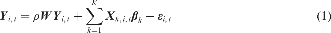

${\mathit{Y}}_{i,t}=\rho \mathit{W}{\mathit{Y}}_{i,t}+{\displaystyle \sum }_{k=1}^K{{\mathit{X}}_{k,i,t}\mathit{\beta }}_k+{\mathit{\epsilon }}_{i,t}$

(1)

where

• $i$ is the BG index $\left(1,\dots ,N\right)$ ;

• $t$ is the index of discrete-time points $\left(1,\dots ,T\right)$ ;

• $k$ is the index of exogenous variables $\left(1,\dots ,K\right)$ ;

• ${\mathit{Y}}_{i,t}$ is the ratio of developed parcels to the total number of parcels in BG _i at time t;

• ${\mathit{X}}_{k,i,t}$ is the $k$ th observation for BG _i at time t;

• $\mathit{W}$ is an $N\times N$ row-standardized spatial weight matrix assumed to be constant over time;

• $\rho$ is the spatial autoregressive coefficient;

• ${\mathit{\beta }}_k$ is the kth regression coefficient;

• $\mathit{\epsilon }$ is the vector of spatial autoregressive disturbances;

The disturbance vector consists of two error terms: (1) $\mathit{\epsilon }$ is a vector of spatially autocorrelated error terms, and (2) $\mathit{v}$ is a vector of independent and individually distributed (iid) error terms, with an expected value of zero and a constant variance

${\mathit{\epsilon }}_{i,t}=\lambda \mathit{W}{\mathit{\epsilon }}_{i,t}+{\mathit{v}}_{i,t}$

(2)

where $\lambda$ is the lag coefficient for the error term $\mathit{\epsilon }$ .

The static panel model in equations (1) and (2) can be modified to account for autoregressive temporal dynamics, whereby previous developments impact future land developments. Temporal lags of the dependent variable can be included in the model to obtain a dynamic model (also called the Autoregressive Regression model), which can be used to forecast future land development. Equations (2) and (3) represent such a DSPD model.

${\mathit{Y}}_{i,t}=\rho \mathit{W}{\mathit{Y}}_{i,t}+{\displaystyle \sum }_{k=1}^K{{\mathit{X}}_{k,i,t}\mathit{\beta }}_k+{\displaystyle \sum }_{s=1}^S{\mathit{Y}}_{i,t-s}\hspace{0.17em}{\mathit{\theta }}_s+{\mathit{\epsilon }}_{i,t}$

(3)

where

• $s$ is the temporal lag index $\left(1,\dots ,S\right)$ ;

• ${\mathit{Y}}_{i,t-s}$ is the sth temporal lag of the dependent variable;

• ${\theta }_s$ is the coefficient of sth temporal lag.

Similarly, a temporal lag of the covariates ( ${\mathit{X}}_{k,i,t-1}$ ) can be included in the model to account for delayed responses in land development dynamics (Eqs. (2) and (4)). This model enables forecasting future land development without the need of a contemporary covariate matrix.

${\mathit{Y}}_{i,t}=\rho \mathit{W}{\mathit{Y}}_{i,t}+{\displaystyle \sum }_{k=1}^K{{\mathit{X}}_{k,i,t-1}\mathit{\beta }}_k+{\displaystyle \sum }_{s=1}^S{\mathit{Y}}_{i,t-s}\hspace{0.17em}{\mathit{\theta }}_s+{\mathit{\epsilon }}_{i,t}$

(4)

The spatial autoregressive coefficient $\left(\rho \right)$ in equation (3) determines the relationship between the dependent variable and a linear combination of neighboring $\mathit{Y}$ values based on the predefined spatial neighborhood matrix $\mathit{W}$ (Anselin, 1988; Ord, 1975). The $\mathit{W}\mathit{Y}$ matrix accounts for spatial dependencies in the dependent variable. This model also controls spatial dependencies through its error term (equation (2)). However, spillover effects through covariates may also affect land development dynamics. The $\mathit{W}\mathit{X}$ matrix, also known as spatial lags of covariates, computes average values of neighboring land characteristics and accounts for spillover effects through the covariate matrix. The $\mathit{W}\mathit{X}\mathit{\gamma }$ is also known as the exogenous interaction effect (See more details in the SF). Adding such effects (while ignoring the temporal dependencies) leads to the Spatial Durbin Model (SDM). Adding the temporal lags to the SDM leads to equation (5)

${\mathit{Y}}_{i,t}=\rho \mathit{W}{\mathit{Y}}_{i,t}+{\displaystyle \sum }_{k=1}^K{{\mathit{X}}_{k,i,t}\mathit{\beta }}_k+{\displaystyle \sum }_{s=1}^S{\mathit{Y}}_{i,t-s}\hspace{0.17em}{\mathit{\theta }}_s+{\displaystyle \sum }_{k=1}^K\mathit{W}{\mathit{X}}_{k,i,t}{\mathit{\gamma }}_k+{\mathit{\epsilon }}_{i,t}$

(5)

where $\mathit{\gamma }$ is a $k\times 1$ vector of regression coefficients for spatially lagged covariates.

Equations (5) and (2) can be combined with

${\mathit{Y}}_{i,t}={\left[\mathit{I}-\mathrm{\rho }\mathit{W}\right]}^{-1}\hspace{0.17em}\left[{\displaystyle \sum }_{\mathrm{k}=1}^K{{\mathit{X}}_{k,i,t}\mathit{\beta }}_k+{\displaystyle \sum }_{\mathrm{s}=1}^S{\mathit{Y}}_{i,t-s}\hspace{0.17em}{\mathit{\theta }}_s+{\displaystyle \sum }_{\mathrm{k}=1}^K\mathit{W}{\mathit{X}}_{k,i,t}{\mathit{\gamma }}_{\mathit{k}}+{\left[\mathit{I}-\mathrm{\lambda }\mathit{W}\right]}^{-1}{\mathit{\epsilon }}_{i,t}\right]$

(6)

where $\mathit{I}$ is an identity matrix of dimension $N\times N$ . Equation (6) demonstrates the non-linear nature of the model.

Conceptualization of the spatial relationships

The DSPD model uses the spatial weight matrix W to conceptualize spatial relationships. Three main methods are used to construct spatial weight matrices: fixed distance, K-nearest neighbors, and contiguity. This study uses the K-nearest neighbors rule to test various spatial conceptualizations (Figure S2 in the SF). The inverse-distance-weight (IDW) method is used to account for potential distance-related spatial spillover effects. The row-standardization method is implemented for all spatial weight matrices to avoid the identification problem in regression models.

Computation of direct and indirect effects

Equation (6) presents the DSPD model incorporating both the spatial interactions of exogenous variables and spatial and temporal lags. Marginal effects based on the spatial structure are constant over time due to the non-varying spatial weight matrix. The marginal effects can be obtained by using the partial derivative of the dependent variable with respect to a given explanatory variable and temporal lags of the dependent variable at time t

$\frac{\partial {\mathit{Y}}_t}{\partial {\mathit{X}}_k}={\left[\mathit{I}-\rho \mathit{W}\right]}^{-1}\left({\mathit{\beta }}_k+{\mathit{W}\mathit{\gamma }}_k\right)$

(7)

$\frac{\partial {\mathit{Y}}_t}{\partial {\mathit{Y}}_{t-s}}={\left[\mathit{I}-\rho \mathit{W}\right]}^{-1}{\mathit{\theta }}_s$

(8)

where ${\mathit{X}}_k$ is the kth column of the covariate matrix $\mathit{X}$ at time t.

Using Equations (7) and (8), average direct, total, and indirect effects can be computed for a given year (LeSage and Pace, 2009; Park et al., 2021). Equations (9), (10), and (12) represent the average direct (ADE), total (ATE), and indirect (ANE) effects of the temporal lags of the dependent variable, respectively

$AD{E}_s={\mathfrak{t}}_{\gamma }\left({\left[\mathit{I}-\rho \mathit{W}\right]}^{-1}\right)\hspace{0.17em}{\mathit{\theta }}_s/N$

(9)

$AT{E}_s={\mathit{\iota }}^{\prime }{\left[\mathit{I}-\rho \mathit{W}\right]}^{-1}\hspace{0.17em}\mathit{\iota }{\mathit{\theta }}_s/N$

(10)

$AN{E}_s=AT{E}_s-AD{E}_s$

(11)

where $\mathit{\iota }$ is a $N\times 1$ vector of ones, ${\mathit{\iota }}^{\prime }$ is the transpose of $\mathit{\iota }$ , and ${\mathfrak{t}}_{\gamma }(.)$ is the trace operator.

Marginal effects for the independent variable can also be computed using the following equations

$AD{E}_k={[\mathfrak{t}}_{\gamma }\left({\left[\mathit{I}-\rho \mathit{W}\right]}^{-1}\right)\hspace{0.17em}{\mathit{\beta }}_k+{{\mathfrak{t}}_{\gamma }\left({\left[\mathit{I}-\rho \mathit{W}\right]}^{-1}\mathit{W}\right)\mathit{\gamma }}_k]/N$

(12)

$\mathit{A}\mathit{T}{\mathit{E}}_{\mathit{k}}={[\mathrm{\iota }}^{\prime }{\left[\mathit{I}-\mathrm{\rho }\mathit{W}\right]}^{-1}\mathrm{\iota }{\mathrm{\beta }}_{\mathrm{k}}+{\mathrm{\iota }}^{\prime }{\left[\mathit{I}-\mathrm{\rho }\mathit{W}\right]}^{-1}\mathit{W}\mathrm{\iota }{\mathrm{\gamma }}_{\mathrm{k}}]/\mathrm{N}$

(13)

$AN{E}_k=AT{E}_k-AD{E}_k$

(14)

The elasticities of the direct and indirect effects can be further computed by multiplying both sides of equation (6) by ${\mathit{X}}_k/{\mathit{Y}}_t$ . Equation (15) represents the elasticities for the kth variable at time t. A similar approach can be applied for the temporal lag of the dependent variable by multiplying both sides of equation (8) by ${\mathit{Y}}_{t-s}/{\mathit{Y}}_t$ . Equation (16) represents the elasticity for the sth temporal variable at time t.

$\frac{\partial {\mathit{Y}}_t}{\partial {\mathit{X}}_k}\hspace{0.17em}\frac{{\mathit{X}}_k}{{\mathit{Y}}_t}=\left[{\left[\mathit{I}-\rho \mathit{W}\right]}^{-1}\left({\mathit{\beta }}_k+{\mathit{W}\mathit{\gamma }}_k\right)\right]\cdot \frac{{\mathit{X}}_k}{{\mathit{Y}}_t}$

(15)

$\frac{\partial {\mathit{Y}}_t}{\partial {\mathit{Y}}_{t-s}}\frac{{\mathit{Y}}_{t-s}}{{\mathit{Y}}_t}={\left[\mathit{I}-\rho \mathit{W}\right]}^{-1}{\mathit{\theta }}_s\cdot \frac{{\mathit{Y}}_{t-s}}{{\mathit{Y}}_t}$

(16)

Data and study area

Florida is one of the fastest-growing U.S. states, with a population of 20.9 million in 2019. In this study, three primary data sources are used: (1) site-specific, proximity, and neighborhood characteristics are derived from the 2019 Florida Parcel Database, published by UF GeoPlan Center (“Florida Parcel Data Statewide,” 2019), where the database consists of 8,995,663 individual parcel records; (2) transportation characteristics are derived from the Florida Department of Transportation (FDOT) traffic records; (3) socio-economic characteristics at the BG level are obtained from the American Community Survey (ACS). These data sets are further discussed below.

Land development characteristics

Land development characteristics are derived from the actual construction year and land use information provided in the statewide parcel-level database. Figure S3 in the SF depicts the number of developed parcels in 2019 and their changes between 2010 and 2019 (an increase of 10.06%). Figure S4 in the SF illustrates the annual changes in the number of developed parcels in BGs by population density category between 2010 and 2019. BGs are grouped into 10 equally sized groups based on population density, where the least dense BGs are assigned to Category 1 and the densest BGs to category 10. Land development rates increased over these 10 years. Less dense BGs experienced higher land development intensity than denser BGs. The average lot size in Florida is 1.51 ha, the median is 0.09 ha, and the standard deviation is 31.62. The distribution of average lot size is heavily skewed to the left.

Proximity and neighborhood characteristics

Using the parcel data, Euclidean distances from parcel centroids to the nearest points of interest and amenities are calculated and averaged at the BG level to capture proximity characteristics (Figure S5 in the SF). In addition, the shares of various land uses within a 3.2 km (2-mile) circular buffer centered at each parcel centroid are also calculated and averaged at the BG level as proxies for neighborhood characteristics (Figure S6 in the SF).

The average distance to the nearest industrial facility from parcels was 1.37 km in 2010, decreasing by 2.47% over the 10 years. The average distance to the nearest educational building was 1.43 miles in 2010, decreasing by 1.89% over the decade. The average agricultural land share within a 3.2-km radius increased from 2.49% in 2010 to 2.63% in 2019. Similarly, the average share of recreational land rose from 1.9% to 1.98%. The average share of single-family residential land was 31.5% in 2019, increasing by 3.8%. Finally, the average percentage of mixed-use land rose from 0.28% in 2010 to 0.29% in 2019.

Traffic volume

Historical annual average daily traffic data between 2010 and 2019 were obtained from the Transportation Data and Analytics Office of the Florida Department of Transportation (FDOT). The perpendicular distance to the closest roadways and the average of Annual Average Daily Traffic (AADT) on the 100 closest road sections from a given BG centroid are computed using the annual data (Figure S7 in the SF). The average perpendicular distance to the nearest main road section was 0.87 km in 2010, and it declined by 36.5% over 10 years. The average AADT increased by almost 20% over the same period.

Socio-economic characteristics

The ACS 5-year estimates provide socio-economic information at the BG level. Socio-economic characteristics for a given year are retrieved from the 5-year ACS survey ending with that year. The average population density has increased from 16.76 to 18.10 (person per hectare). The ratio of minority populations, including African-Americans, Asians, and people of two or more races, also increased. The number of occupied housing units rose by 6.79%. The average student ratio decreased by 6.6%, from 22.2% to 20.1%. The average employment ratio increased by 4.3%. The average share of employees commuting by car declined by 1.4%. Finally, the share of financed housing units using mortgage loans decreased from 34.9% to 30.7%.

Descriptive statistics

Table S2 in the SF presents descriptive statistics for the variables used in the regression models over 2010–2019. The table reports mean and standard deviation statistics for each year. The only time-invariant variables are lot area and variance of lot areas. Therefore, these variables are not included in the table. The mean and standard deviation of the average lot area at the BG level are 8.73 and 369.8 ha, respectively. The average lot area variance is 4370.5 with a standard deviation of 190262.4.

Results

This section presents the statistical analysis results based on data covering 11,394 BGs in Florida, after removing BGs located in coastal areas and without any parcels and 21 BGs because of missing information. All statistical analyses are conducted using R software packages (spdep and splm). Spatially lagged covariates and temporally lagged dependent variables are prepared in the R software before inputting them into the spdep and splm packages. Before conducting regression analyses, pair-wise Pearson’s correlations are computed to identify moderate and strong linear associations between independent variables. Significant correlations among independent variables violate the independence assumption. Figure S8 in the SF presents the statistically significant pair-wise Pearson’s correlations for the independent variables. The home occupancy ratio, distance to industrial complexes, and distance to education facilities are moderately correlated with many variables. Therefore, these three variables are excluded from further statistical analysis. The only exception is made for the variance of parcel areas, which is strongly correlated with the average parcel area.

Testing different spatial weight matrix rules

Different spatial weight matrix rules based on the K-nearest neighbors method are tested using the DSPD model with a temporal lag to find the optimal spatial weights for further analysis after excluding the previously identified independent variables which are moderately correlated with many variables. The spatial autoregressive coefficient ( $\rho$ ), Bayesian Information Criteria (BIC), Akaike’s Information Criteria (AIC), Adjusted R², average Moran’s I test for residual spatial autocorrelation, and the number of statistically insignificant variables are presented in Table S3 in the SF for the tested models. The average Moran’s I test statistics are obtained by averaging the estimated Moran’s I test values over time. Based on the BIC and AIC values, the spatial weight matrix using the 200^th nearest neighbor rule (without IDW) is considered the most appropriate. This model has also the smallest spatial autocorrelation in the standardized residual.

Exploratory regressions

After identifying the appropriate spatial weight matrix, multiple model specifications are tested to determine the best-fit model for the data. Using the set of explanatory variables used in the previous section, different temporal and spatial configurations are tested during this exploratory regression analysis phase. Table S4 in the SF represents statistics from the tested models to evaluate the goodness-of-fit. Nonspatial and spatial models without temporal lag are tested to obtain a baseline for spatio-temporal models. Model combinations with contemporaneous or temporally lagged covariates, spatially lagged covariates, the number of temporal lags (up to 2), and spatial autocorrelation in the error term are tested.

AIC and BIC values close to zero indicate favorable model specifications. Models ignoring temporal or spatial lags perform poorly. Model 8 has AIC and BIC values closest to zero, and its adjusted R² value is 0.9909, slightly smaller than the maximum value. Model 8 has the smallest Moran’s I test value for standardized residual that is important for the model assumptions. Another important criterion is the number of insignificant variables. Model 8 estimates statistically significant relationships except for one parameter, whereas the other models often provide insignificant results. Therefore, Model 8 is further investigated. It accounts for temporally lagged covariates and two temporal lags. In this model, the coefficient of the lagged mixed-use land ratio variable is statistically insignificant. Therefore, this variable is dropped from the model, and the final results are presented in Table 2. Removing the insignificant variable does not significantly change the model’s goodness-of-fit. The lagged covariates indicate that previous characteristics impact contemporaneous land developments. The positive ρ of 0.0156 indicates that an increase in the land development ratios in neighboring BGs leads to a rise in the land development ratio of the given BG. Spatial and temporal lag coefficients reveal important land development dynamics. The one-lag spatial and temporal coefficient ( ${\theta }_1$ ) of 1.4339 shows that land developments that occurred in the previous year in neighboring BGs raise the potential land development in the given BG. However, the ${\theta }_2$ of −0.4485 indicates that land developments that occurred 2 years ago in neighboring BGs reduce the potential land development in the given BG. This suggests that the earlier development discourages new land development due to insufficient vacant land in the BG.

Table 2.

Model 8 results excluding the insignificant variable.

Variable	Estimate	Std. Error	t-value	Pr(>|t|)
(Intercept)	0.00230	0.00041	5.56047	<0.00001	***
Site-specific characteristics
Average lot area	>-0.00001	<0.00001	−3.48924	0.00048	***
Lot area variance	<0.00001	<0.00001	1.85349	0.06381
Socio-economic characteristics
Lagged population density	−0.00003	<0.00001	−11.50699	<0.00001	***
Lagged ratio of non-white population	−0.00191	0.00022	−8.69390	<0.00001	***
Lagged ratio of students	0.00196	0.00050	3.93283	0.00008	***
Lagged employment ratio	0.00267	0.00042	6.33579	<0.00001	***
Lagged ratio of financed units	0.00096	0.00029	3.26074	0.00111	**
Lagged ratio of workers commuting by car	−0.00078	0.00039	−1.96633	0.04926	*
Neighborhood characteristics
Lagged share of single-residential parcels	−0.00001	<0.00001	−2.06072	0.03933	*
Lagged share of recreational areas	0.00003	0.00002	1.90159	0.05723	.
Lagged share of agricultural lands	−0.00005	0.00001	−4.33691	0.00001	***
Transportation characteristics
Lagged perpendicular distance to a road	−0.00052	0.00007	−7.26635	<0.00001	***
Average of AADT	−0.01743	0.00282	−6.17406	<0.00001	***
Spatial and temporal lag coefficients
${\theta }_1$	1.43392	0.00344	416.774	<0.00001	***
${\theta }_2$	−0.44854	0.00341	−131.706	<0.00001	***
$\rho$	0.01560	0.00079	19.8010	<0.00001	***

 Significance levels: Model statistics:

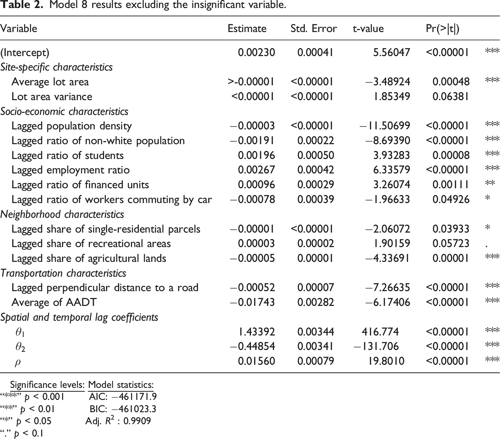
“***” p < 0.001   AIC: −461171.9

“**” p < 0.01    BIC: −461023.3

“*” p < 0.05    Adj. R² : 0.9909

“.” p < 0.1

Since the development ratio ranges between 0 and 1, this limited response variable may not be suitable for the DSPD model. To evaluate the impacts of this approach on parameter estimations and model statistics, the dependent variable is transformed using the logit function ( $\mathrm{l}\mathrm{o}\mathrm{g}\mathrm{i}\mathrm{t}\left[p\right]=\log \left[p/1-p\right]$ ). The logit transformation helps to expand the limited range 0–1 (Massey and Fong, 1990). During the transformation, an epsilon (0.0001) is added to zeros and subtracted from ones to avoid taking logarithms of 0. All regression analyses are repeated using the transformed dependent variable, and the results are presented in the SF (Tables S5 and S6). Model results based on the transformed response variable are similar to the initial results. The main difference is the statistical significance of a few variables (see Table S7 in the SF). Finally, the suitability of BG-level data for LUC modeling is further investigated by using subdivisions of BGs as spatial unit (Figure S9 in the SF). The results of the regressions with subdivision data are presented in Table S8 in the SF, and display a higher adjusted R² as compared to Model 8 due to a larger number of observations. However, parameters’ signs are the same in both analyses. Also, parameters’ significance and magnitudes are not changing drastically, which indicates that BG-level data is suitable for land use change modeling in Florida.

Direct and indirect effects

Model 8 results are further analyzed in this section. Table 3 presents the average elasticities of the explanatory variables’ direct, indirect, and total effects, including their significance levels. The dependent variable’s first temporal lag ( ${\theta }_1$ ) has the highest impact on a BG development potential. As the previous year’s ratio of developed parcels in a given BG increases by 1%, this ratio is expected to rise by 1.42%, with a minimal indirect impact. The second temporal lag ( ${\theta }_2$ ) is the second most influential factor: a 1% increase in the ratio of developed parcels 2 years earlier implies an expected decrease of 0.44%. These findings indicate that the most recent developments more strongly attract new developments. Note that a 1% increase in the ratio of developed parcels at the BG level represents approximately 8 parcels or 13 ha of land based on mean values of lot counts and sizes. A 1% increase in lot size results in a slight drop of 0.00051% in the expected ratio of developed land. A 1% raise in lot size variance results in a 0.00015% increase in the expected developed land ratio. These results indicate that smaller lot sizes and recent developments encourage new development.

Table 3.

Average elasticities of the direct, indirect, and total impacts based on Model 8 estimates between 2012 and 2018.

Variable	Direct	Indirect	Total
Site-specific characteristics
Average lot area	−0.00051**	<0.00001***	−0.00051***
Lot area variance	0.00013**	<0.00001***	0.00013***
Socio-economic characteristics
Lagged population density	−0.00055***	−0.00001***	−0.00056***
Lagged ratio of non-white population	−0.00063***	−0.00001***	−0.00064***
Lagged ratio of students	0.00062***	0.00001***	0.00063***
Lagged employment ratio	0.00166***	0.00002***	0.00168***
Lagged ratio of financed units	0.00044***	0.00001***	0.00045***
Lagged ratio of workers commuting by car	−0.00098***	−0.00001***	−0.00100***
Neighborhood characteristics
Lagged share of single-residential parcels	−0.00035***	−0.00001***	−0.00036***
Lagged share of recreational areas	0.00008***	0.00000***	0.00008***
Lagged share of agricultural lands	−0.00021***	<0.00001***	−0.00021***
Transportation characteristics
Lagged perpendicular distance to a road	−0.00111***	−0.00001***	−0.00112***
Average AADT	−0.00044***	−0.00001***	−0.00044***
Temporal lag coefficients
${\theta }_1$	1.41848***	0.02250***	1.44098***
${\theta }_2$	−0.44111***	−0.00700***	−0.44811***

 Significance levels:

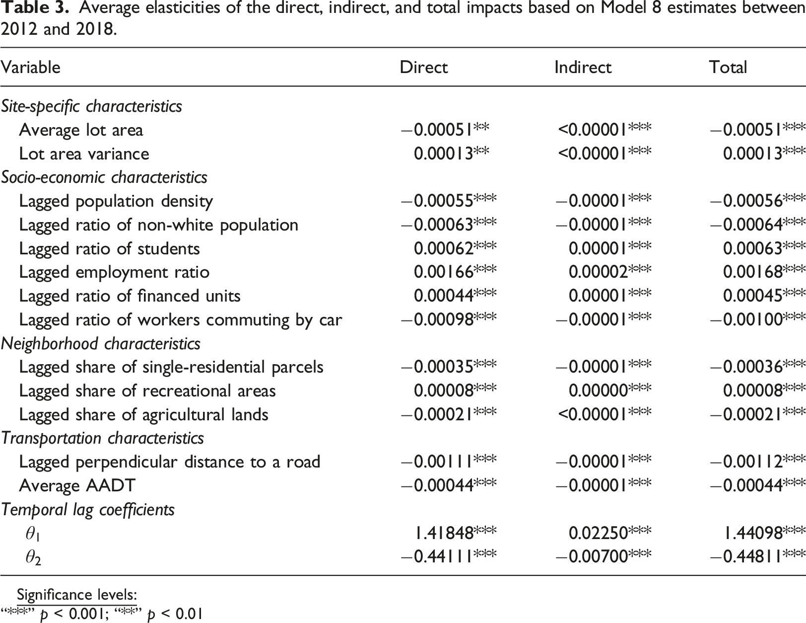
“***” p < 0.001; “**” p < 0.01

The model also captures other essential dynamics. Among the socio-economic factors, the lagged employment ratio most strongly affects the land development potential. A 1% rise in the previous year’s employment ratio increases the expected land development ratio by 0.0017%. At the same time, higher employment rates in neighboring BGs are also positively associated with land development but with a much weaker effect. On the other hand, a 1% change in the previous year’s student population ratio in each BG results in a 0.0006% rise in the expected development. In contrast, the expected development decreases slightly as the ratios of student population increase in neighboring BGs. A higher proportion of the employed and student populations supports an active real estate market. A 1% increase in the lagged non-white population ratio decreases the expected percentage of land development by 0.0006%. Because the non-white population ratio is generally related to income, areas with a larger non-white population are likely to have lower development potential. A 1% rise in the lagged population density results in a 0.0006% decline in the expected development ratio, but the same surge in neighboring BGs increases the development potential. This suggests that relatively less developed areas surrounded by denser populations are attractive locations for further development. A 1% increase in the lagged ratio of financed homes results in a 0.0004% rise in development, and there is also a positive indirect association between neighboring financed home ratios and land development. High rates of financed units are signs of active buyers in the market. Finally, a 1% increase in the lagged percentage of workers commuting by car decreases the expected ratio of developed land by 0.001%. Higher commuting rates by car may indicate potential traffic congestion, which may discourage new urban growth.

The model also captures the effects of specific neighborhood characteristics. A 1% increase in the lagged shares of single-family, agricultural, and recreational areas in each BG decreases the expected development by 0.0004% for single-family units and 0.0002% for agricultural development. However, it increases the expected development by 0.00008% for recreational areas. The corresponding indirect effects are much smaller than the direct effects. Considering the analyzed period, the existing agricultural lands are in peripheral regions, and such locations require longer commutes and are less desired for new land developments. An increase in the current single-family residential areas in BG areas reduces the potential for urban growth due to fewer available vacant lots. Finally, recreational lands benefit nearby areas, including landscape views, clean air, and activity spaces. Therefore, these areas are attractive places for new urban developments.

Finally, the model results underline the importance of transportation infrastructure and traffic volumes. A 1% decrease in the lagged distance from a given BG to the nearest road section increases the expected development by 0.0011%. This result confirms the importance of road accessibility for real estate development. However, a 1% increase in average traffic volume results in a 0.0004% decline in growth, suggesting that the adverse effects of high traffic volumes reduce development potential.

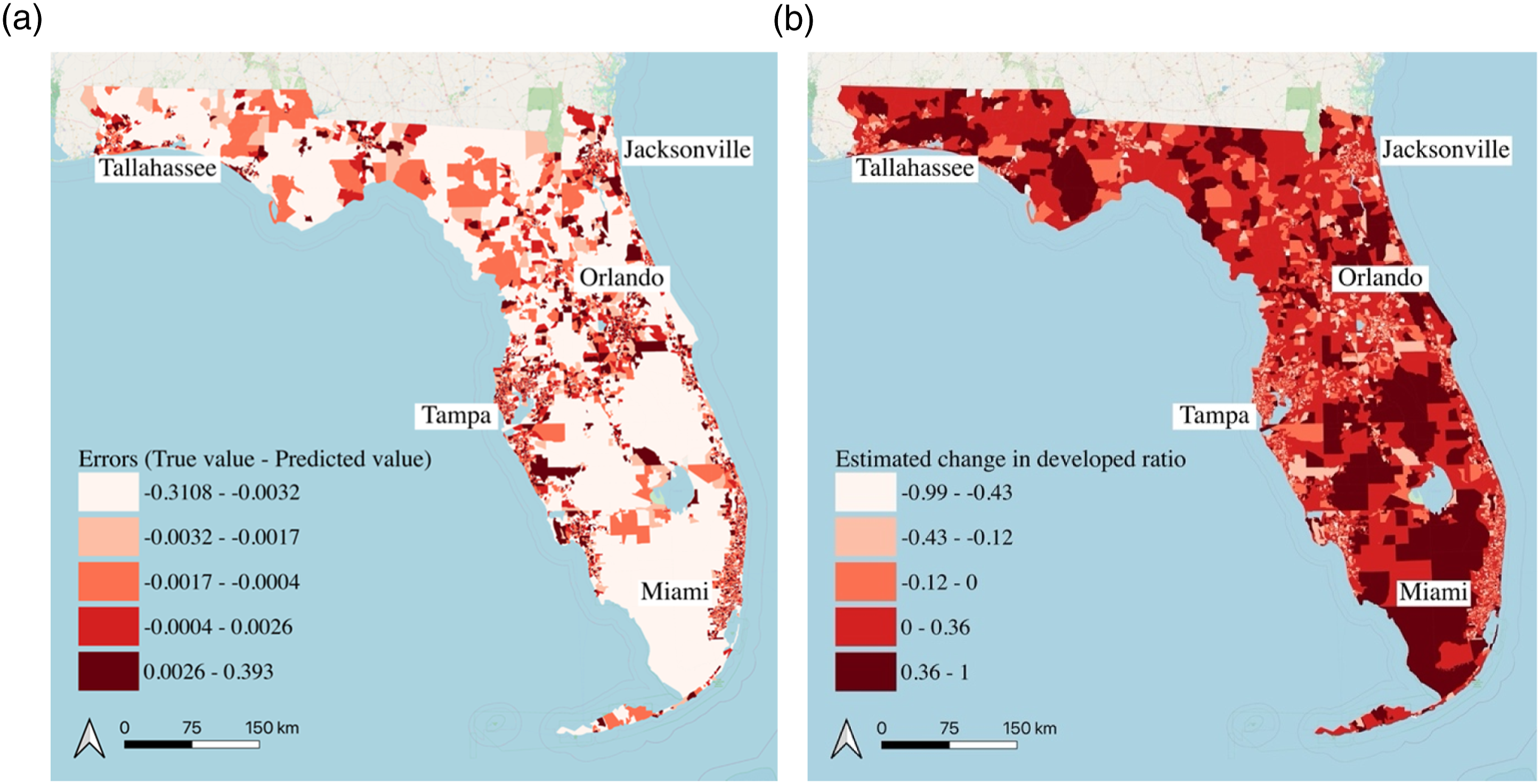
Predictive ability of the model

In this study, 2019-year data is used for model validation. Therefore, 2019-year data is not included in prior regression analyses. As LUC models can be used for predicting future land developments, Model 8 is used to predict growth in 2019 based on the situation in 2018. Equation (17) estimates the expected land development at time t+1 (2019) using the existing (2018) covariate matrix. Since the DSPD is a regression model, R² statistics can be used for prediction accuracy (equation (18)). The prediction accuracy is computed as 99.1%. Figure 1 presents (a) the difference between actual and estimated values and (b) estimated changes in the developed ratios in 2019. The model predicts fewer developments in dense urban areas like Jacksonville, Miami, Tampa, Orlando, and Tallahassee (Figure 1(b)). However, the model expects urban growth potential near environmentally sensitive areas south of Orlando and west of Miami.

${\widehat{\mathit{Y}}}_{i,t+1}={\left[\mathrm{I}-\mathrm{\rho }\mathit{W}\right]}^{-1}\hspace{0.17em}\left[{\displaystyle \sum }_{k=1}^{\mathrm{K}}{\mathit{X}}_{k,i,t}\hspace{0.17em}{\mathit{\beta }}_k+{\displaystyle \sum }_{s=1}^2{\mathit{Y}}_{i,t+1-s}\hspace{0.17em}{\mathit{\theta }}_s+{\mathit{\epsilon }}_{i,t+1}\right]$

(17)

$R^2=1-\frac{\frac{1}{N}{\displaystyle \sum }_i^N{({\mathit{Y}}_i-{\widehat{\mathit{Y}}}_i)}^2}{Var\left(\mathit{Y}\right)}$

(18)

Figure 1.

(a) Differences between actual and estimated values and (b) Changes in developed ratio from 2018 to 2019.

Discussion

In this section, the findings of this study are compared with those of previous studies to evaluate further the appropriateness of the proposed framework for urban growth modeling. Previous studies (see Table S9 in the SF) do not include the ratios of minorities and students, financed housing units, workers commuting by car, and average AADT (or any type of traffic variable). The impact of parcel size is estimated to be negative in this paper and studies by Carrión-Flores and Irwin (2004) and Tepe and Guldmann (2020), while Nahuelhual et al. (2012) and Tepe and Guldmann (2017) indicate a positive association between urban growth and parcel size. These contradictory results suggest non-linear relationships between parcel size and urban development. According to several previous studies, population density positively affects growth (Gaur et al., 2020; Huang et al., 2009; Jokar Arsanjani et al., 2013; Tepe and Guldmann, 2017). However, Carrión-Flores & Irwin (2004) and Hu and Lo (2007) indicate negative associations, as does this study. The employment ratio is consistently estimated to have a positive effect (Deng and Srinivasan, 2016; Hu and Lo, 2007).

The share of single-family residential areas is negatively associated with urban growth in this study and in the regression results of Arsanjani et al. (2013) and Tepe and Guldmann (2017), in contrast to the positive effects in Carrión-Flores and Irwin (2004) and Tepe and Guldmann (2020). Tepe and Guldmann (2020) provide insight into the impacts of the share of residential areas, where the percentage of residential areas is positively associated with single-family residential parcels and other residential units. However, the relationship is negative with other land uses. The impacts of recreational areas on land development are always positive (Jokar Arsanjani et al., 2013). In this study, the effect of the agricultural land share is assessed as negative, consistent with the results in Deng and Srinivasan (2016) and Tepe and Guldmann (2020). However, other studies display negative associations (Carrión-Flores and Irwin, 2004; Irwin et al., 2003; Liao and Wei, 2014). Irwin et al. (2003) state that the positive sign is unexpected. There is a consensus on the sign of distance to major roads among previous studies (Carrión-Flores and Irwin, 2004; Hu and Lo, 2007; Huang et al., 2009; Jokar Arsanjani et al., 2013; Lavalle et al., 2011; Liao and Wei, 2014; Nahuelhual et al., 2012; Tepe and Guldmann, 2017, 2020). Spatial autocorrelation and the first temporal lag coefficient are also positively associated with land developments in several studies (Bhat et al., 2015; Deng and Srinivasan, 2016; Ferdous and Bhat, 2013; Huang et al., 2009; Nahuelhual et al., 2012; Tepe and Guldmann, 2017, 2020).

In this study, spatial weight matrices are constructed based on a predefined rule conceptualizing spatial relationships, similar to the previous studies discussed in this section. There is no theoretical basis for creating spatial relationships in land-use change modeling. Therefore, the conceptualization rule is identified based on an empirical analysis that minimizes the spatial autocorrelations in the residual. The presence of spatial dependency in the residual violates the statistical independence of observations (LeSage and Pace, 2009).

Conclusions

A DSPD model has been proposed and applied, including site-specific, proximity, neighborhood, socio-economic, and transportation variables. This model explicitly accounts for spatial and temporal dependencies. The overall model accuracy is almost 99%, and the prediction accuracy is 99.3%. Using historical data and temporally lagged covariates allows this model to predict future urban growth. A robust land development model can provide essential information to practitioners and policymakers about potential urban expansions. Such information will enable them to mitigate unexpected outcomes and effectively manage resources appropriately. For instance, the proposed modeling framework can predict land developments near environmentally sensitive areas.

Computations of marginal effects provide insight into the commonly used proxy information in LUC models. Proximities to major road infrastructure and employment ratio are the most impactful factors in urban growth after historical conditions in neighboring BGs. The results further emphasize the importance of incorporating temporal dimensions in LUC models.

There are four significant limitations to the proposed model: (1) Inability to control more complex non-linear relationships in land development dynamics; (2) Use of only continuous response variables, while LUC models often contain discrete-response variables; (3) Scalability of the modeling framework because of computational challenges in computing the inverse of the spatial weight matrix, as required for parameter estimations and predicting future urban growth; (4) accounting for random and fixed effects in the DSPD modeling framework. These limitations provide future research opportunities to contribute to the existing literature.

Supplemental Material

Supplemental Material - History, neighborhood, and proximity as factors of land-use change: A dynamic spatial regression model

Supplemental Material for History, neighborhood, and proximity as factors of land-use change: A dynamic spatial regression model by Emre Tepe in Environment and Planning B: Urban Analytics and City Science.