
Abstract

Introduction (AC)
I translate the 1913 article Das Gesetz der Bevölkerungskonzentration by the German physicist Felix Auerbach to English. I also reproduce the figures of Auerbach with English explanations of some key information. 1 Although Auerbach’s path-breaking contribution to the field of human and economic geography has started to be widely recognized, 2 his article has never been translated before to the best of my knowledge.
In his article, Auerbach argues that the city size distributions of Germany, 3 Great Britain, the U.S.A. etc. approximately satisfy the equation pn p = k where k is a constant and n p is the rank of the city with population p when cities are ranked by population from largest to smallest. 4 Auerbach’s argument is based on a graph where he plots the rank-population product of cities pnp on the vertical axis against their rank n p on the horizontal axis and finds that, from some relatively small value for n p onward, pnp fluctuates within a narrow range around a constant value. Auerbach then points out that pn p = k implies that the number of cities of size larger or equal p is inversely proportional to p. This follows as the rank n p of a city with population p is also the number of cities with population larger or equal p and pnp = k implies n p = kp−1. In 1925, the mathematician and physical scientist Alfred J. Lotka rewrote the relationship n p = kp−1 proposed by Auerbach as log n p = log k−log p. 5 Lotka then reexamined Auerbach’s hypothesis for US cities in 1920 by plotting the log rank of cities on the vertical axis against their log size on the horizontal axis and calculating the ordinary-least-squares regression slope. His slope estimate is −0.93, close to the −1 implied by Auerbach’s hypothesis. The log-log formulation of Auerbach’s hypothesis is employed in the literature since then (e.g. Xavier Gabaix, Zipf’s Law for Cities: An Explanation, Quarterly Journal of Economics, 114(3), 739-767, 1999). In Appendix Figure 1, I reexamine Auerbach’s original data on German cities in 1910 using Lotka’s log-log approach and find an ordinary-least-squares regression slope of −1.15. 6
Later the relationship between n p and p documented by Auerbach became known as Zipf’s law for cities, named after the linguist and philologist George K. Zipf who discussed a wide range of applications of power laws—including their application to city size distributions (Zipf, 1949). 7 Interestingly, Auerbach, in his concluding paragraph, had already speculated that the law he proposed for city size might have applications in the natural sciences, geography, statistics, economics, etc., such as the distribution of wealth or mountain heights. Zipf recognized Auerbach’s earlier contribution, see the short biography of Auerbach by Diego Rybski (Rybski, 2013). 8
Translation of The Law of Population Concentration by Felix Auerbach
At first glance, the facts of human life do not seem to conform to specific general laws as the phenomena of nature do. But, as statistics teaches us, the difference—due to the more complex relationships driving the facts of human life— is just a minor one and one must only learn to read statistical data to be able to draw general conclusions. Sometimes this yields interesting and odd laws.
Such a law concerning population statistics will be presented here and illustrated with examples. This law makes it possible to characterize the distribution of the population within a geographic area—a country for example—in a new and, at least in some respects, more accurate way than possible up to now.
The population living within a geographic area may be distributed in many different ways. In some regions, the population lives in individual farms or small farming villages. Other regions may have larger villages, towns, cities, or even global cities. There is only a handful of global cities in the world and none in many countries, quite a few more major cities, and there is a large number of medium-sized cities. The number of towns, small towns, and villages goes into the hundreds and thousands. For example, in Germany, there is just one global city if one relies on administrative borders and two global cities if one considers their topographic extent; the number of big cities is around 50 and the number of small cities around 200; and there are more than 2000 country towns and nearly 100,000 villages.
Let us sort the places where people live in a country (or any geographic area, like a province or a continent) according to the number of inhabitants and give each place a rank number, starting with 1 for the place with the most inhabitants. Let us also assign to each place its number of inhabitants. Finally, let us multiply the rank number of each place with its number of inhabitants. To avoid unnecessarily large numbers, we can drop the last 5 digits, i.e. round the number down to the nearest hundred thousand. This number will be called the “characteristic product” of the place or the “absolute concentration” of the population—abbreviated by A.K. (The reasons for referring to the number as absolute concentration will become clear soon.)
Population and absolute concentration across German cities.
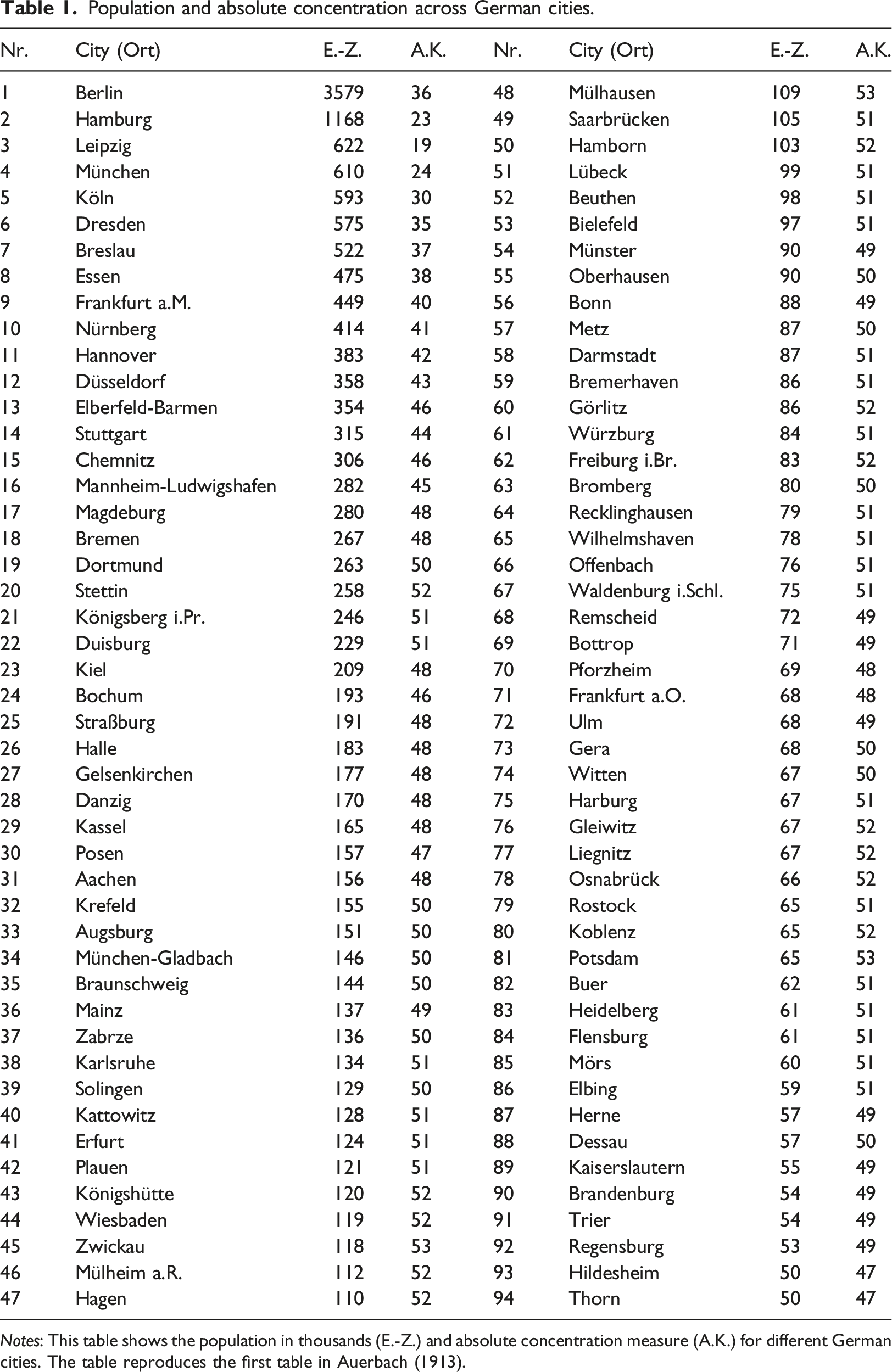
Notes: This table shows the population in thousands (E.-Z.) and absolute concentration measure (A.K.) for different German cities. The table reproduces the first table in Auerbach (1913).
Looking at Table 1—or, even more clearly, at Figure 1—we can see that the absolute concentration (A.K.). fluctuates strongly in the beginning. But fluctuations become smaller very soon and then the absolute concentration is surprisingly constant, rather than rising or falling. In fact, from the rank number 15 onward, absolute concentration fluctuates only between the extrema of 45 and 53. One can therefore justify calculating the average, which is 47.8, and thereby obtains an absolute concentration for not just a single place but a geographic area, in our case Germany. It should be noted that if one were to extend the list of places even further, nothing essential would change. For example, Germany has 236 places with at least 20,000 inhabitants and 481 places with at least 10,000 inhabitants. If one stops at places with a population of 20,000, one obtains an absolute concentration A.K. of 47.2; if one stops at a population of 10,000, one obtains 48.1. In any case, it is better to stop earlier, because the absolute concentration of a geographic area is meant to capture the concentration of its population, and very far down the list one can hardly speak of population concentration. Population and absolute concentration.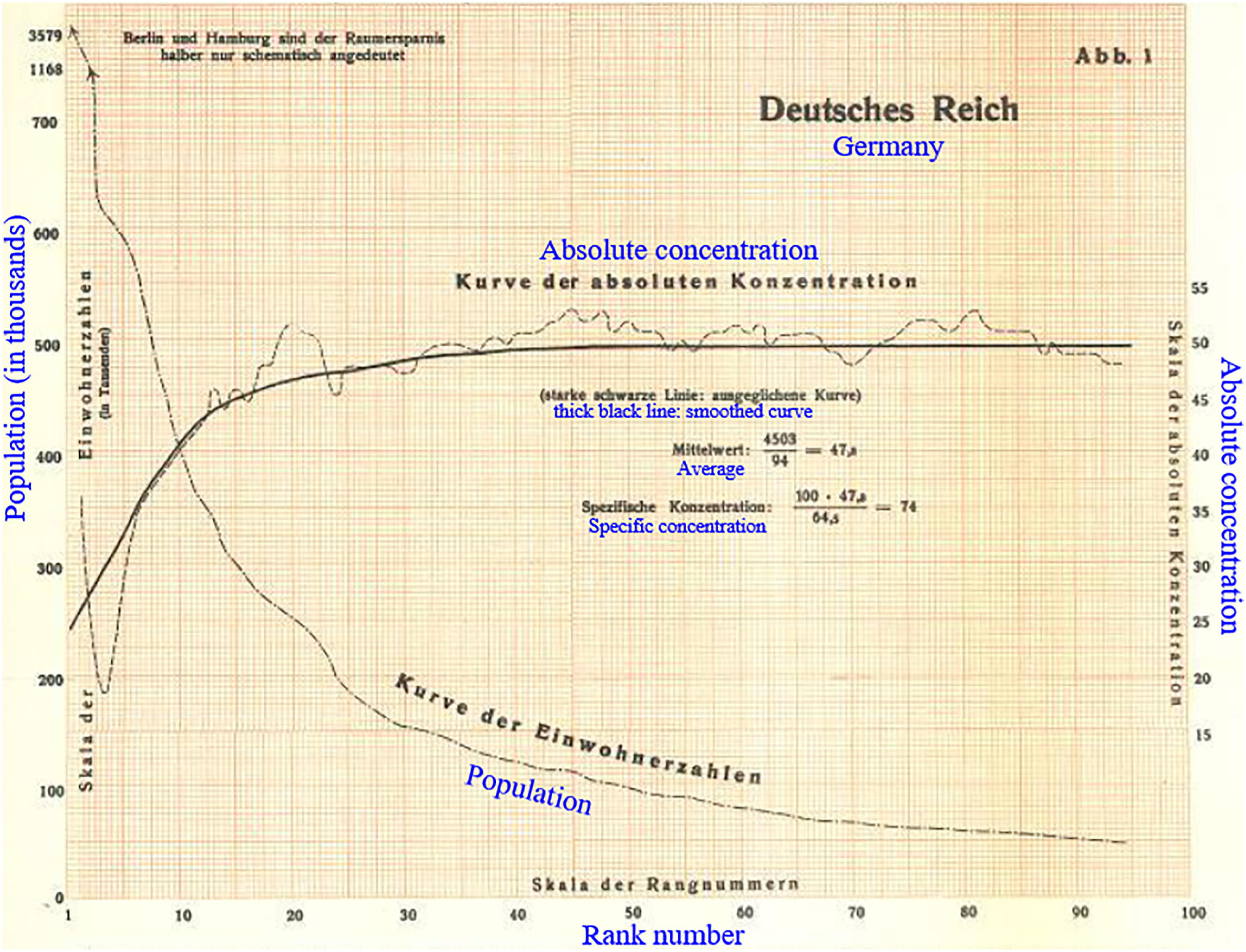
The number 47.2 can therefore be used to characterize the population concentration of Germany. Of course, if one wants to draw comparisons with other countries, the absolute concentration has to be adjusted to take into account that it will increase proportionally with the total population size of a country. We must therefore divide the absolute concentration A.K. for a geographic region by its total population. For convenience, total population will be measured in hundreds of millions. For Germany, whose population is 64.6 million, we therefore have to divide its absolute concentration by 0.645 and we get—rounded down—the final number 74. This number will be called the reduced characteristic product, or better, the “specific concentration” of the population and abbreviated with Sp.K.
The specific concentration of the population in a country has a meaning which differs clearly and substantially from similar measures that have been used for a long time. This is especially true for the most closely related concept, the average population density of a country. A country can have a high population density but a low specific concentration if the population lives in many, closely located villages. And the relationship between population density and specific concentration is reversed if a country has a small population but the population is concentrated in a few bigger cities. This is not to deny that average population density and specific concentration will go together in many cases. The measure of average population density has, by the way, another drawback known to all statisticians and geographers: that one does not really know how to treat big cities, whether one should include them or exclude them up to a certain size class; neither approach yields an unclouded picture of the situation. These and other difficulties are completely avoided using the concept of specific concentration, precisely because it is based on a law that provides a universal constant for all places of a geographic area.
With these considerations we have gotten ahead of establishing the facts; we still have to provide evidence that the proposed law is also valid for other geographic areas. First, for other countries. Figure 2 shows the curves of specific concentration for seven of the most important countries. As can be seen moving from left to right along the horizontal axis, the rank number where the specific concentration starts being approximately constant differs across countries and the approximation is not always equally perfect (which could be easily explained). But the specific concentration of countries can always be finally calculated with sufficient precision. Table 2 lists the average absolute concentration A.K. and the specific concentration Sp.K. for the countries in Figure 2 plus some others. Countries are listed from larger to smaller specific concentration and the population data is from the latest available census, all conducted between 1909 and 1912. Suburbs and city centers have again been combined into metropolitan areas in a cautious manner. Specific concentration of the population across countries. Concentration measures across countries. Notes: This table shows the absolute concentration measure (A.K.) and specific concentration measure (Sp.K.) for different countries. The table is based on the second table in Auerbach (1913). The German country names are in parentheses.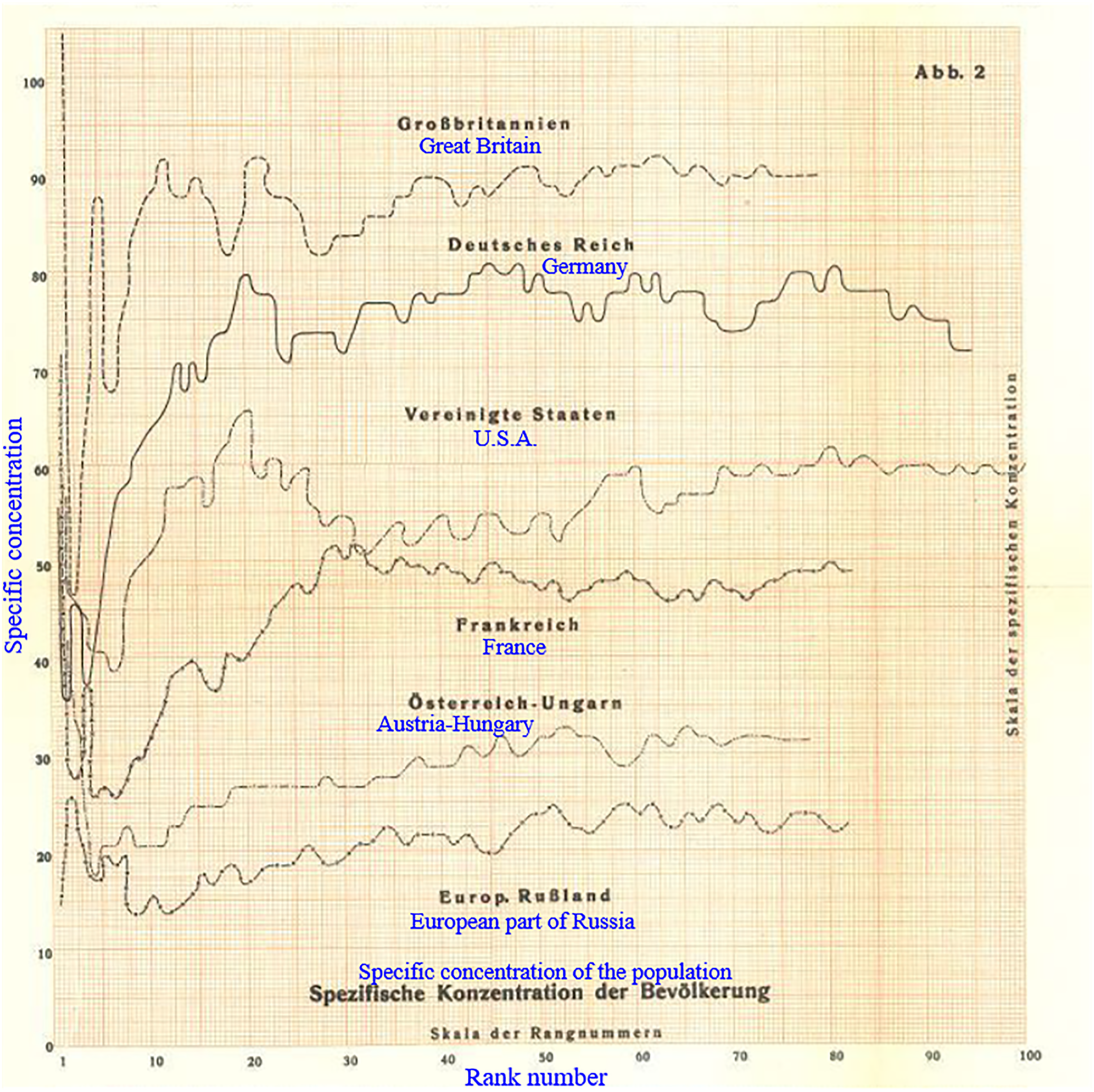
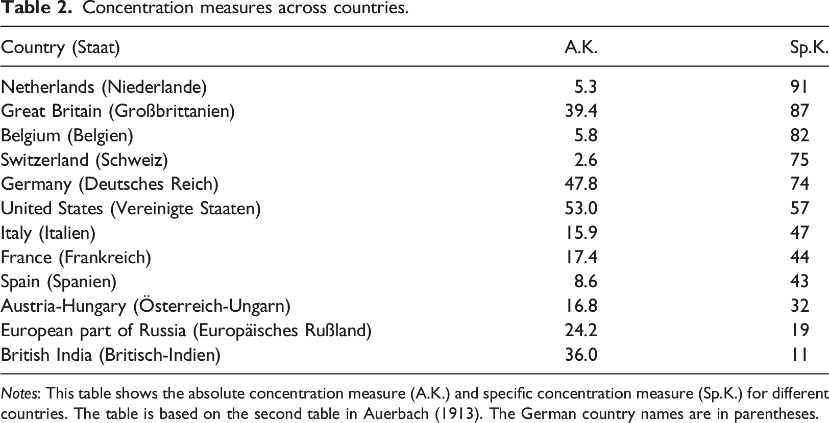
The specific concentration Sp.K. of the population in Great Britain is eight times that of British-India, although its population density is only twice that of British-India; the reason is that India, while densely populated, has only a very small part of its population living in medium-size or large cities. And while Italy is somewhat more densely populated than Germany, the specific concentration of Germany is considerably larger. The comparison of Italy and France shows how general our characterization is and how little specificities turn out to matter, even if they are quite extreme; although France has a city of 3 million inhabitants while Italy does not have any city with more than 1 million inhabitants, Italy’s specific concentration is still somewhat larger than that of France.
Concentration measures across German provinces.
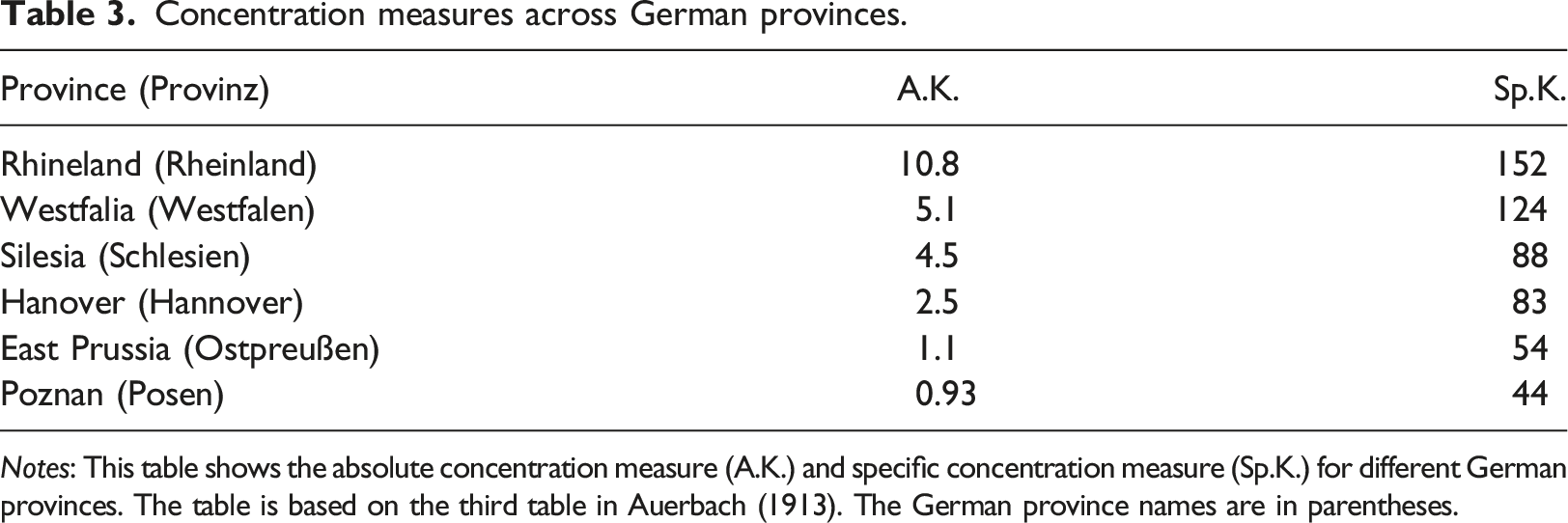
Notes: This table shows the absolute concentration measure (A.K.) and specific concentration measure (Sp.K.) for different German provinces. The table is based on the third table in Auerbach (1913). The German province names are in parentheses.
One can also examine much larger geographic areas, for example Europe as a whole. In this case one obtains slowly increasing absolute concentration up to around rank number 30 (population 520,000). From there onward, absolute concentration becomes constant apart from small fluctuations. The average A.K. of the 334 places with at least 50,000 inhabitants is 169; if one divides this number by 4.32—the population of Europe measured in hundreds of millions—one obtains a specific concentration of 39. As one can see, due to the influence of places in Russia, this number is substantially below the specific concentration of most European countries.
A last example illustrates changes over time in the concentration of the population. As is well known, the concentration of the population has been increasing in most countries, although at a different pace. Figure 3 shows the curves of absolute concentration A.K. for Germany in 1895, 1900, 1905 and 1910. Now the population of places is obtained using administrative borders for simplicity. The figure shows quite clearly that absolute concentration captures more than average population density. That the curves move up over time is a consequence of increasing population density; but that the curves move up so strongly is also due to the increasing concentration of the population. One only has to look at the included numbers for specific concentration Sp.K., which still grow considerably between 1895 and 1910 although the effect of increasing population density has been eliminated by rescaling. To put it differently, in these 15 years, the population density has increased from 52.3 to 64.5, i.e. by 23%; absolute concentration has increased from 28.7 to 49.5, i.e. by 72%; and specific concentration has increased from 55 to 77, i.e. by 40%. Concentration of the population in Germany.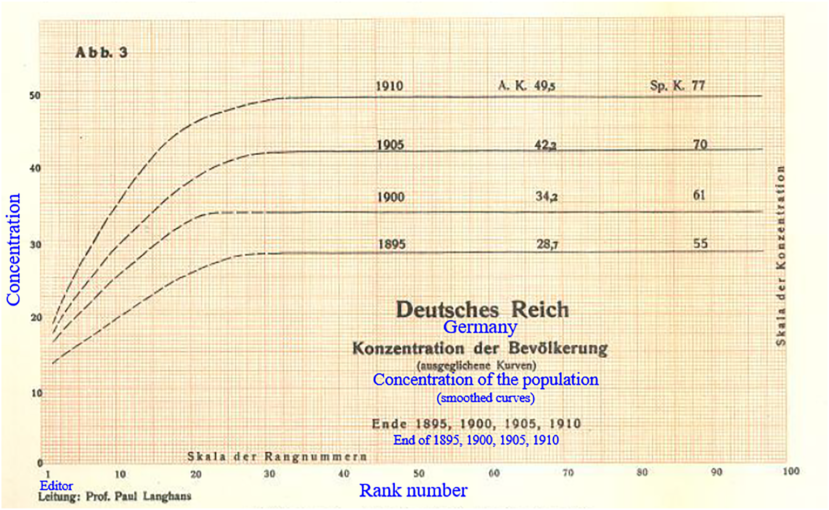
Although the law has further applications, these brief remarks should be enough to stimulate further research by experts who will, I have no doubt, draw conclusions that are deeper than mine.
There are some additional aspects that I want to touch upon in my conclusion. At this point, the law is purely empirical, like so many laws in the natural sciences. Of course, the next step is to understand what is behind it. This task becomes much easier if one first realizes that the law is a special case of a much more general law, which can be applied to the most diverse problems of the natural sciences, geography, statistics, economics, etc. The more general law can be formulated approximately as follows. Suppose one orders n individuals according to a certain property p in descending order and stops either at the rank number n1, or at n2, or—–more generally—–at rank number nx, with the associated property p having fallen to the values p1, p2, and px. Then a certain relationship exists between nx and px. In our special case, the relationship is particularly simple; the equation is nx ⋅ px = constant. Or in words, the number of places is inversely proportional to the population of the smallest of these places. In other cases, the law will be less simple. Consider the following two examples. The first concerns the heights of the summits of a mountain range. In this case, the relationship is much weaker as the highest summit usually surpasses the next-highest ones just by a little. The second example concerns the distribution of wealth across the inhabitants of a country. In this case, the relationship between rank number and personal wealth is much stronger, as the number of individuals is inversely proportional to the square of the minimum wealth in the group. That is, there are four times as many half-millionaires as millionaires, not just twice as many. The theoretical question is now where these variations of the law come from. Here I can only offer the following hints. The simpler the circumstances, the weaker will the relationship be in general. This is because a single driving force is exhausted more easily than two or more. The formation of summits is essentially just a question of the force that formed mountains and this force did not reach beyond a certain limit. Circumstances are more complex when it comes to the formation of cities and even more complex when it comes to the accumulation of wealth.
Of course, all of these are only suggestions and examples to clarify the meaning of what has been discussed here from a more theoretical perspective.
Supplemental Material
Supplemental Material - The Law of Population Concentration
Supplemental Material for The Law of Population Concentration by Antonio Ciccone in Environment and Planning B: Urban Analytics and City Science
Footnotes
Acknowledgements (Antoni Ciccone)
I am very grateful to Gilles Duranton, Xavier Gabaix, Benjamin Moll, and Diego Rybski for their comments. A special thanks to Benjamin Moll and Diego Rybski for checking the translation.
Declaration of conflicting interests (AC)
The author(s) declared no potential conflicts of interest with respect to the research, authorship, and/or publication of this article.
Funding (AC)
The author(s) disclosed receipt of the following financial support for the research, authorship, and/or publication of this article: This work was supported by the Financial support by the German Research Foundation (DFG) through CRC TR 224 (project A04) is gratefully acknowledged.
Supplemental Material (AC)
Supplemental material for this article is available online.
Notes (AC)
Translator Biography (AC)
Appendix
Log-log plot using Auerbach’s data for German cities in 1910. Notes: The data is from Felix Auerbach’s Das Gesetz der Bevölkerungskonzentration in Petermanns Geographische Mitteilungen, 59, 74-76, 1913. There are 94 cities in the graph. The robust standard error of the ordinary-least-squares slope (−1.15) is 0.03.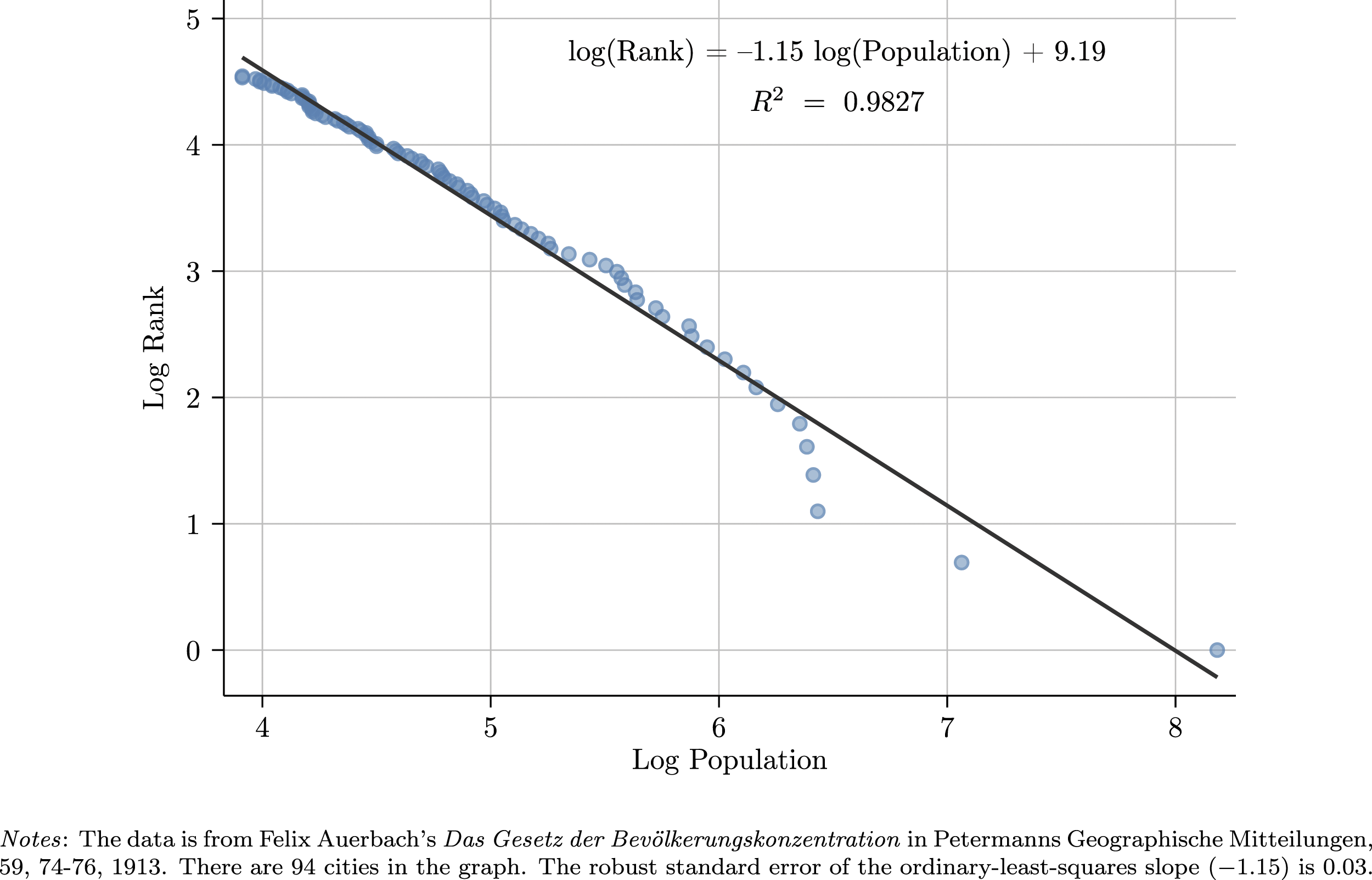
Supplementary Material
Please find the following supplemental material available below.
For Open Access articles published under a Creative Commons License, all supplemental material carries the same license as the article it is associated with.
For non-Open Access articles published, all supplemental material carries a non-exclusive license, and permission requests for re-use of supplemental material or any part of supplemental material shall be sent directly to the copyright owner as specified in the copyright notice associated with the article.